vent â besides the assumption of caustic-free data â the necessity to make .... in Eq. 9, for 100 iterations for λ decreasing from λ1 = 4 to λ100 = 0.02 for the ...
4248
ROBUST CURVELET-DOMAIN DATA CONTINUATION WITH SPARSENESS CONSTRAINTS FELIX J. HERRMANN Department of Earth and Ocean Sciences, University of British Columbia, Vancouver, BC, Canada
Abstract A robust data interpolation method using curvelets frames is presented. The advantage of this method is that curvelets arguably provide an optimal sparse representation for solutions of wave equations with smooth coefficients. As such curvelets frames circumvent – besides the assumption of caustic-free data – the necessity to make parametric assumptions (e.g. through linear/parabolic Radon or demigration) regarding the shape of events in seismic data. A brief sketch of the theory is provided as well as a number of examples on synthetic and real data.
Linear data interpolation Data continuation has been an important topic in seismic processing, imaging and inversion. For instance, our ability to accurately and artifact-free image or predict multiples, as part of surface related multiple elimination, depends for a large part on the availability of densely and equidistantly sampled data. Unfortunately, constraints on marine and land acquisitions preclude such a dense sampling and several efforts have been made to solve issues related to aliasing and missing traces. Typically, data continuation approaches involve some sort of a variational problem that aims to jointly minimize the L2 -mismatch, between measured and interpolated data, and an independent penalty functional (regularization term) on the interpolated data, which we will call the model. For quadratic penalty functionals, the solution for the variational problem [see e.g. 3] 1 (1) m ˆ = arg min kd − Pmk22 + λkDmk22 m 2 can be written explicitly as �−1 T m ˆ = P∗ P + λD∗ D P d. (2) In this expression, d is the (weighted) acquired vector with the missing data; m the regularly sampled data and P the picking matrix, which puts to zero the missing data samples/traces. The symbol ∗ denotes the adjoint. Since the picking matrix is not invertible, Eq. 1 contains an additional penalty term which regularizes the inverse problem of data interpolation. The λ-weighted penalty term typically imposes smoothness on the model with D some type of sharpening operator such as a (fractional) Laplacian, i.e. D· = ∆α · with α ≥ 0. For a specific choice of regularization, Eq. 1 corresponds to kriging or spline interpolation.
Non-linear sparseness-constrained interpolation Despite its elegance, Eq. 1 has a number of serious drawbacks amongst which (i) the inherent non-stationarity of seismic data, which makes it difficult to define the appropriate sharpening operator D defining the covariance operator C· = D∗ D·; (ii) the notion that wavefronts are typically oscillatory in the normal direction to the wavefront and smooth in the direction along the wavefronts, which is not trivially accounted for; (iii) wavefronts are sparse, i.e. seismic data can be thought of as a superposition of limited number of events, e.g. plane waves or solutions to some sort of modeling operator such as the adjoint of the migration operator. Relatively recently these observations have led to a non-linear model/transform-driven reformulation of Eq. 1 given by 1 m ˆ = arg min kP (d − Lm) k22 + λkmkpp with 1 ≤ p < 2. (3) m 2 In this expression, L stands for either a modeling operator – such as the adjoint of the (linear/parabolic) Radon, the apex-shifted Radon or the demigration operator [16, 15] or for a generic orthogonal basis-function decomposition such as the Fast Fourier Transform [11, 5, 12]. As long as events in the data roughly behave as the columns in L, good interpolation results have been obtained by solving the above system (e.g. with the method of Iterated Re-weighted Least Squares IRLS [9]). Unfortunately, events in less-than-ideal data are not likely to behave exactly according to the columns of L. Moreover, the singular vectors associated with the solution of Eq. 3 tend to spread globally even though the `1 -norm invokes ’spikyness’ in these vectors and the solution. To limit the dependence on assumptions regarding the shape of the events, we propose to use curvelet frames [2], which consist of localized multi-scale & angular elements that can be interpreted as local plane waves which are smooth in one direction and oscillatory in the other.
Figure 1: Left: Curvelet partitioning of the frequency plane [courtesy to 2]. Right: Illustration showing that curvelet coefficients are small when curvelets are not alligned with an event. Non-linear sparseness-constrained interpolation with curvelet frames The method presented in this paper is similar to the approach of Eq. 3. Major difference, however, is that we replace the modeling or Fourier/Radon transform operators by a generic frame composition defined by the curvelet frame. Compared to the model-driven approaches, our approach has the advantage that (i) curvelet frames are known to be sparse for seismic data (they obtain close to optimal non-linear approximation rates for seismic data); (ii) no assumptions are made regarding the type of events present in the data. For example, events no longer need to be close to parabolic or linear as is the case for parabolic and linear Radon. The events can lie on arbitrary but piece-wise smooth (twice-differentiable) curves [13]. Before going into detail on how to apply the method, let us first provide more details on curvelet properties. We then proceed by showing how to compute the `1 -minimization by iterative thresholding. We conclude by applying our method to synthetic as well as real data.
Why Curvelets How do curvelets obtain such a high non-linear approximation rate? Without being all inclusive [see for details 2], the answer to this question lies in the fact that curvelets are • • • •
multi-scale, i.e. they live in different dyadic corona in the FK-domain (see Figure 1). multi-directional, i.e. they live on wedges within these corona. anisotropic, i.e. they obey the following scaling law width ∝ length2 . 1 directional selective with # orientations ∝ √scale .
• local both in (x, t) and (k, f ). • a numerically tight frame with moderate redundancy and an explicit construction exists for the adjoint that equals the pseudo inverse: CT · = C† ·, yielding kf k22 = cT c with c = Cf the curvelet coefficients of f and C the curvelet transform. For more detail on curvelet frames refer to [8, 7].
Sparsity-enhancing frame expansions by iterative thresholding For orthogonal basis functions, soft thresholding on noisy coefficients y [10, 4] x ˆ = Sλs (y) ,
(4)
1 x ˆ = arg min ky − xk22 + kxk1 x 2
(5)
solves component-wise the following variational problem
with kxk1 = kxk11 the `1 -norm. Unfortunately, curvelets are frames which means that Eq. 4 is no longer equivalent to Eq. 5. Following recent work by [4] and [14], we replace Eq. 4 by an iterative thresholding procedure. At each iteration, evaluation of � cm = Sλs m cm−1 + T∗ (d − Tcm−1 ) (6) yields an approximate estimate for the coefficient vector. For large enough number of iterations, the solution from Eq. 6 converges to the following variational problem on the coefficients 1 ˆ c = arg min kd − Tck22 + λkck1 . (7) c 2 In Eq. 6, d is the possibly noisy data vector, T∗ the curvelet transform, T its pseudo-inverse and cm the estimated coefficient vector after m iterations with possibly decreasing thresholds λm . Eq. 6 converges to a sparse set of curvelet coefficients that reconstruct the image [4, 14]. By setting the λm ’s proportional to the noise-level, the iterations in Eq. 6 yield the denoised coefficients from which the denoised data can be reconstructed by taking the inverse curvelet transform.
Data continuation with curvelets As shown independently within both the seismic (see e.g. [11, 12, 16]) and image (see e.g. [6]) processing communities, Eq. 7 can simply be adapted to the situation of missing data by including the picking operator 1 ˆ c = arg min kP (d − Tc) k22 + λkck1 , c 2
(8)
which corresponds to replacing 6 by
� cm = Sλs m cm−1 + T∗ P(d − Tcm−1 ) .
(9)
This expression is used to generate the examples of the next section by setting the maximal number of iterations to m = 100 while linearly decreasing λm .
Examples Above iterative method is applied to synthetic as well as real data. Results for a synthetic shot-record using the iteration defined in Eq. 9, for 100 iterations for λ decreasing from λ1 = 4 to λ100 = 0.02 for the noise-free case and λ100 = 3σ for the standarddeviation σ = 2 case, are listed in Fig. 2. Our method is clearly able to achieve good results on synthetic data even for the noisy case. Similarly, our results for a real shot record as depicted in Fig. 3 are satisfactory. In this case, λ1 = 4 and λ1 00 = 0.05.
Discussion and conclusions The success of our approach can heuristically be explained by arguing that curvelets act as an “unconditional basis” for seismic data (both primaries and multiples), which we consider to be generated by the (repeated) action of a scattering operator. Whenever a basis is unconditional, one finds that (i) the data’s covariance is near diagonal in the basis and (ii) the norm (say `p ) shrinks when shrinking the coefficients. The argument that curvelets can be considered to be close to an unconditional basis for seismic data derives from the work on function spaces by [13] and from Theorem 1.1 of [1] which states that Green’s functions are nearly diagonalized by curvelets. Consequently, seismic data can be represented by a sparse coefficient vector rendering our data-continuation method to be (i) effective for caustic-free seismic data with events on arbitrary curves; (ii) robust under additive possibly colored noise (see other contribution by the author to these Proceedings). Our method, can relatively easily be generalized to 3-D; speeded up by using more intelligent `p -solvers. Main challenge lies in extending the method to cases where there are caustics.
Acknowledgments The author would like to thank the authors of the Digital Curvelet Transform (Candes, Donoho, Demanet and Ying). This work was carried out as part of the SINBAD project with financial support, secured through ITF (the Industry Technology Facilitator), from the following organizations: BG Group, BP, ExxonMobil and SHELL. Additional funding came from the NSERC Discovery Grant 22R81254.
References [1] E. J. Cand`es and L. Demanet. The curvelet representation of wave propagators is optimally sparse. 2004. Preprint: http://www.acm.caltech.edu/ demanet. [2] E. J. Cand`es and F. Guo. New multiscale transforms, minimum total variation synthesis: Applications to edge-preserving image reconstruction. Signal Processing, pages 1519–1543, 2002. [3] J. Claerbout. Earth soundings analysis: Processing versus inversion. Blackwell Scientific publishing, 1992. [4] I. Daubechies, M. Defrise, and C. de Mol. An iterative thresholding algorithm for linear inverse problems with a sparsity constrains. CPAM, pages 1413–1457, 2005. [5] A. Duijndam, A. Volker, and P. Zwartjes. Reconstruction as efficient alternative for least-squares migration, pages 1012– 1015. Soc. of Expl. Geophys., 2000. [6] M. Elad, J. Starck, P. Querre, and D. Donoho. Simulataneous Cartoon and Texture Image Inpainting using Morphological Component Analysis (MCA). 2005. [7] F. Herrmann and P. Moghaddam. Sparseness- and continuity-constrained seismic imaging with curvelet frames. 2005. [8] F. J. Herrmann and P. Moghaddam. Curvelet-based non-linear adaptive subtraction with sparseness constraints. In Expanded Abstracts, Tulsa, 2004. Soc. Expl. Geophys. [9] L. Karlovitz. Construction of nearest points in the `p , p even and `1 norms. J. Approx. Theory, 3, 1970. [10] S. G. Mallat. A wavelet tour of signal processing. Academic Press, 1997. [11] M. Sacchi and T. Ulrych. Estimation of the discrete fourier transform, a linear inversion approach. Geophysics, 61(04):1128– 1136, 1996. [12] M. Schonewille and A. Duijndam. Parabolic radon transform, sampling and efficiency. volume 66, pages 667–678. Soc. of Expl. Geophys., 2001. [13] H. Smith. A Hardy space for fourier integral operators. J. Geom. Anal., 7, 1997. [14] J. L. Starck, M. Elad, and D. Donoho. Redundant multiscale transforms and their application to morphological component separation. Advances in Imaging and Electron Physics, 132, 2004. [15] D. Trad, T. Ulrych, and M. Sacchi. Latest views of the sparse radon transform. Geophysics, 68(1):386–399, 2003. [16] D. O. Trad. Interpolation and multiple attenuation with migration operators. Geophysics, 68(6):2043–2054, 2003.
0
-2000
0
2000
0
0.5
0.5
1.0
1.0
1.5
1.5
2.0
2.0
-2000
(a) Missing data
0
-2000
0
0
2000
(b) Interpolated data
2000
0
0.5
0.5
1.0
1.0
1.5
1.5
2.0
2.0
(c) Noisy missing data
-2000
0
2000
(d) Denoised & interpolated data
Figure 2: Synthetic examples of curvelet data continuation applied to a synthetic shot record. (a) Shot record with missing traces; (b) Interpolation result. (c) Noisy (standard-deviation σ = .2 data with missing traces. (d) Denoised and interpolated data. These examples show that the curvelet data continuation gives good results even for noisy data.
50
100
150
200
250
50
4
4
5
5
6
6
7
7
(a) Missing data
100
150
200
250
(b) Interpolated data
Figure 3: Real example of curvelet data continuation applied to a real shot record with missing data. (a) Shot record with missing traces; (b) Interpolation result.