2017 Asia-Pacific International Symposium on Aerospace Technology, Seoul, Korea
4D Trajectory Modeling for ATC Simulation Hyuntae Jung* and Keumjin Lee Department of Air Transport, Transportation and Logistics, Korea Aerospace University, Goyang-si, Korea
-----------------------------------------------------------------------------------------------------------------------------------------------------------------------------------------------------------------------------------------------------------------------------------------------------------
Abstract To maximize utilization of airspace and airport, various next generation ATM (Air Traffic Management) concepts are being introduced. Especially, the concept of 4D TBO (Trajectory Based Operation) is expected to revolutionize air traffic system when its fully operational. In prior to integrate such concepts into the real operational environment, its attribute must be validated through simulation. In this paper, the air traffic control simulation model suitable to emulate both conventional and 4D trajectory environments is introduced. Based on aircraft performance parameter based on Eurocontrol BADA 3, the 4D trajectory is defined as 4-dimensional cubic Bezier spline. Each curve consisting the spline is generated from waypoints with constraints such as altitude, airspeed and climb/descent rate corresponding to each waypoint. After being validated its feasibility with aircraft performance parameters provided by BADA, the generated 4D trajectory is defined as reference trajectory. Then each aircraft is controlled to follow the reference trajectory with proportional control method. Three guidance modes are being introduced: dynamic, static and manual; according to in which variable to take control among defined reference trajectory. Finally, the comparison between generated 4D trajectory and the result of simulation with both control modes will be included. With this work, the simulation is expected to be flexible and realistic to be used in various of ATM researches. Keywords: Air Traffic Control Simulator, 4D Trajectory Modeling, Trajectory Based Operation -----------------------------------------------------------------------------------------------------------------------------------------------------------------------------------------------------------------------------------------------------------------------------------------------------------
1. Introduction
Nomenclature 𝑥 𝑦 ℎ 𝑣 𝑚 𝜓 𝜙 𝛾 𝑡 𝑎 𝑔0 𝑝 𝜌 𝑆 𝑇 𝐷 𝐿 𝐶𝐷 , 𝐶𝐿 𝐹 𝐶𝑓,1 , 𝐶𝑓,2 𝜏 𝑃𝑘 (𝜏) 𝑊𝑃𝑗
= = = = = = = = = = = = = = = = = = = = = = =
longitude of the aircraft position latitude of the aircraft position aircraft altitude TAS (true airspeed) aircraft mass aircraft heading bank angle flight path angle time acceleration gravitational acceleration air pressure air density wing surface thrust drag lift drag and lift coefficient specific fuel consumption fuel consumption coefficient curve parameter kth segment jth waypoint
𝑃𝑟𝑖 𝑙 𝜆0 , 𝜆1 𝑑 𝜃 𝑣𝑤 , 𝜓𝑤
= = = = = =
ith reference point arc length Bezier curve optimization parameter distance to reference point bearing to reference point wind speed and direction
Air transport is one of the rapidly growing industry, and experienced its highest growth over the last five years with the benefit of recent low oil prices. Especially, 5.6% of annual RPK (revenue passenger-kilogram) growth is expected in Asia-Pacific market while 3.4% and 2.4% per annum were expected in European and North American market respectively [1]. However, because of the limited capacity of existing airports and airspaces, the excessive demand over capacity is causing air traffic delay inflicting economic and environmental loss. In order to increase the capacity of existing infrastructure by maximizing its utility, numbers of ATM (Air Traffic Management) concepts and technologies are being studied and developed. Especially, the concept of 4D TBO (Trajectory Based Operation) is expected to transform conventional clearance-based air traffic system into trajectory-based system by optimizing, sharing and managing aircraft trajectory. By adopting TBO, it is expected to reduce operation cost from minimizing constraints and uncertainty of flight [2]. The Trajectory Based Operation (TBO) was developed to maximize the efficiency of the flight operation by defining, sharing and negotiating aircraft trajectories within user preference and operational constraints. In current radar surveillance based air traffic management system, ATCO (Air Traffic Controller) issues clearance to each aircraft to
* Presenting
& Corresponding Author: Master Student,
[email protected], Member, KSAS. 1
2017 Asia-Pacific International Symposium on Aerospace Technology, Seoul, Korea
guide its path satisfying aircraft separation. However
operation as well as renovating whole system.
especially in the high traffic situation, due to the
More importantly, it is required to validate its
uncertainty in predicting aircraft positions ahead, and the
effectiveness, efficiency and reliability before putting such
absence of DST (Decision Support Tool) that processes
newest concepts into real operation. Simulation is one of
real-time flight data into optimal flight path, it becomes a
most used methods for assessing and analyzing such
serious challenge for ATCO to calculate and assign
technologies
optimized flight path to every aircraft instantly. Due to such
environment. Even though numbers of air traffic control
difficulties, even if airline might plan flight path to be the
simulators with commercial or research purpose were
most fuel efficient, radar vectoring poses an inevitable
developed, still some simulators are offering limited
inefficiency in redrawing such flight path which makes
accessibility, flexibility or compatibility to apply such
operation cost unnecessarily high. Also, pilots or airlines
technologies and conduct a simulated test for ATM
have difficulties in assimilating ATC intention completely.
researches.
Through
the
recent
but
realistic
air
traffic
CNS/ATM
With this motivation, this paper introduces the 4DT (4D trajectory) modeling and simulation. Based on aircraft
Management),
(System
in
simulated
(Communication, Navigation, Surveillance and Air Traffic SWIM
development
in
Information
performance parameter and dynamics from Eurocontrol
Management) and DST, the concept of TBO has emerged
Wide
BADA (Base of Aircraft Data) 3 and Total Energy Model
and expected to handle the problems.
[3], the 4DT is defined as 4-dimensional cubic Bezier spline. The simulation model is made up of generating and validating reference trajectory from flight plan or radar track data, and controlling aircraft to follow the predefined reference trajectory with given guidance mode. The simulation is designed to be flexible, realistic and able to support both TBO and non-TBO flights so that it could be used in various ATM researches.
2. 4D Trajectory Model 2.1. Reference Trajectory Modeling The whole aircraft trajectories, starting from take-off to landing were defined as 4-dimensional Bezier splines. These splines have smoothness of C1 continuity; the splines are defined as the sets of the cubic Bezier curves jointed end to end with continuous first derivates (but not necessarily second order differentiable). By this mean, the trajectory can be split into the sets of flight path, starting from one point to another. Fig. 1. The comparison between conventional clearance-based ATC and trajectory based ATC In TBO, such inefficiency could be mitigated by predefining user preferred trajectory, usually referred as “Reference Trajectory” or “Business Trajectory”, then validating the trajectory that satisfies operation constraints and free of conflicts. If there is any conflict, through the negotiation with ATCO, the user and ATCO reach to modified “Agreed Trajectory” which satisfies operation constraints while reflecting the interest of user as much as
Here, the lateral flight path from one waypoint to next waypoint is defined as “segment”, which is expressed as a cubic Bezier curve. In contrast, the vertical path and speed profile is expressed as linear Bezier curve (or just linear function). With given 4 vertices: start point, end point, and 2 control points, the flight segment is defined in cubic Bezier curve form as follows: 3 𝑃(𝜏) = ∑3𝑖=0 ( ) 𝜏 𝑖 (1 − 𝜏)3−𝑖 𝑃 𝑖 , 𝜏 ∈ [0, 1] (1) 𝑖 = (1 − 𝜏)3 𝑃0 + 3𝜏(1 − 𝜏)𝑃1 + 3𝜏 2 (1 − 𝜏)𝑃2 + 𝜏 3 𝑃3
possible. The progress toward trajectory based operation will contribute enhancing the efficiency of individual
In Eq. (1), 𝜏 is the curve parameter within the bound
2017 Asia-Pacific International Symposium on Aerospace Technology, Seoul, Korea
between 0 and 1; (𝜏 = 0) indicates the start of the curve,
When the initial conditions such as position, altitude,
and (𝜏 = 1) indicates the end of the curve. 𝑃0 is the start
airspeed and heading at the waypoint, and parameters such
point, 𝑃3 is the end point, and 𝑃1 & 𝑃2 are the control
as 𝑡𝑟 , 𝜆0 and 𝜆1 are given, the flight segment is
points defining shape of the curve. Each lateral position
generated through Eq. (1) to Eq. (7). Fig. 2. shows the
(longitude and latitude) of control points are expressed as
example of various curves with elapsed flight time: 𝑡𝑟 =
follows [4]:
500, 1000, 2000 and 4000 seconds respectively. Fig. 3. visualizes how 4DT is defined with the parameter (𝜏).
𝑃0 = [
𝑥(𝜏 = 0) ] 𝑦(𝜏 = 0)
cos(𝜓0 ) ] sin(𝜓0 ) cos(𝜓1 ) cos(𝛾) 1 𝑃2 = 𝑃3 + (𝜆1 (𝜏 − 1) − ) 𝑙 [ ] 3 sin(𝜓1 ) cos(𝛾) 𝑥(𝜏 = 1) − 𝑣𝑤 𝑡𝑟 cos(𝜓𝑤 − 𝜋) 𝑃 =[ ] { 𝑘,3 𝑦𝜏 = 1) − 𝑣𝑤 𝑡𝑟 cos(𝜓𝑤 − 𝜋) 1
𝑃1 = 𝑃0 + (𝜆0 𝜏 + ) 𝑙 [ 3
(2)
In Eq. (2), 𝑥 and 𝑦 represent longitude and latitude, 𝜓0 and 𝜓1 represent the headings of the aircraft in 𝑃0 and 𝑃3 . 𝑙 is the arc length of the curve. 𝑡𝑟 represents the elapsed flight time in the segment. 𝑣𝑤 and 𝜓𝑤 are speed and direction of the wind respectively. 𝛾 is the vertical 𝜆0
flight angle.
and 𝜆1
are the curve parameters
determining the curve shape and curvature.
Fig. 2. The example of generated segment based on elapsed flight time (𝒕𝒓 = 𝟓𝟎𝟎, 𝟏𝟎𝟎𝟎, 𝟐𝟎𝟎𝟎 𝐚𝐧𝐝 𝟒𝟎𝟎𝟎 sec)
The vertical flight path and speed profile are defined in linear form, or first-order Bezier curve. The altitude and
The end point (𝑃3 ) of the segment coincides with the start
TAS (true airspeed) of the segment are expressed as
point (𝑃0 ) of the next segment. After drawing every segment,
following equations:
the 4D trajectory is being generated by joining each segments end to end. The introduced 4D trajectory model is
ℎ(𝜏) = (1 − 𝜏) ∙ ℎ(𝜏 = 0) + 𝜏 ∙ ℎ(𝜏 = 1)
(3)
𝑣(𝜏) = (1 − 𝜏) ∙ 𝑣(𝜏 = 0) + 𝜏 ∙ 𝑣(𝜏 = 1)
(4)
used in modeling reference trajectory in the simulation. The detailed 4DT generation and validation process is discussed in chapter 3.1.
Similarly, ℎ and 𝑣 represent altitude and true airspeed, where (𝜏 = 0) and (𝜏 = 1) indicate the start and the end of the segment. The curve parameter, 𝜏 can be computed with flight time (𝑡) by followings: 𝜏(𝑡) =
𝑠(𝑡)
, 𝑤ℎ𝑒𝑟𝑒 {
𝑙
𝑠(0) = 0 𝑠(𝑡𝑟 ) = 𝑙
(5)
Where 𝑡 is the time spent flying the segment, and 𝑠(𝑡) is arc length from 0 to 𝑡. Thus, 𝜏(𝑡) represents the ratio of flown arc length in time 𝑡, compared with whole arc length (𝑙). With following Eq. (6) and Eq. (7), 𝜏 can be derived from flight path angle and airspeed over time. 𝑑𝜏(𝑡) 𝑑𝑡
1
𝑑𝑃(𝜏)𝑇
𝑙 = ∫0 √
𝑑𝜏
=
∙
𝑑𝜏(𝑡) 𝑑𝑠
𝑑𝑃(𝜏) 𝑑𝜏
∙
𝑑𝑠(𝑡) 𝑑𝑡
=
𝑡
𝑣(𝑡) 𝑙
𝑑𝜏 = ∫0 𝑟 𝑣(𝑡) cos(𝛾) 𝑑𝑡
(6)
(7)
Fig. 3. The parameter (𝒙, 𝒚, 𝒉, 𝒗) of segment defined as cubic Bezier curve
2017 Asia-Pacific International Symposium on Aerospace Technology, Seoul, Korea
2.2. Aircraft Dynamics: Total Energy Model
The drag (𝐷) and lift (𝐿) can be computed from drag
The TEM (Total Energy Model) is used as aircraft dynamics in the simulation. TEM equates the rate of work
coefficient (𝐶𝐷 ) and lift coefficient (𝐶𝐿 ) provided by BADA with following equations:
done by forces acting on the aircraft to the rate of increase 𝐶𝐿 =
in potential and kinetic energy. (𝑇 − 𝐷)𝑣 = 𝑚𝑔0
𝑑ℎ 𝑑𝑡
+ 𝑚𝑣
2𝑚𝑔0
(16)
𝜌𝑣 2 𝑆 cos(𝜙)
𝐶𝐷 = 𝐶𝐷,0 + 𝐶𝐷,2 ∙ (𝐶𝐿 )2
𝑑𝑣
(8)
𝑑𝑡
(17)
1
𝐷 = 𝐶𝐷 𝜌𝑣 2 𝑆
(18)
2
Where 𝑇 stands for thrust, 𝐷 for drag, 𝑚 is aircraft mass
and
𝑔0
is
gravitational
acceleration.
By
independently controlling two variables among thrust (𝑇),
Here, 𝜌 represents air density defined in ISA and 𝑆 is the wing surface area of the aircraft. Drag coefficient (𝐶𝐷 ), lift coefficient (𝐶𝐿 ) and wing surface (𝑆) are provided in
𝑑ℎ
airspeed (𝑣) and rate of climb or descent ( ), Eq. (8) can
BADA aircraft performance data. As the fuel is being
be used to calculate the other variable. Although there are
consumed, the aircraft mass ( 𝑚 ) changes as well. The
other models that simulate aircraft movement in the
change of the aircraft mass is expressed with specific fuel
microscopic level [5], because of its low complexity, the
consumption ( 𝐹 ). Depending on the engine type, the
TEM is considered as more suitable for an air traffic control simulator observing overall flow of the traffic. Moreover,
equation of fuel consumption is defined as a function of thrust (𝑇), airspeed (𝑣) and coefficients (𝐶𝑓,1 , 𝐶𝑓,2 ) defined
since we assumed that path angle ( 𝛾 ) change is
in BADA as well.
𝑑𝑡
instantaneous, TEM can be expressed as Gamma-Command 𝑚̇ = −𝐹(𝑇, 𝑣)
Model as followings [6]: (𝑗𝑒𝑡) 𝛾̇ =
𝐿 cos(𝜙) 𝑚𝑣
−
𝑔0 cos(𝛾) 𝑣
𝐿 cos(𝜙) − 𝑚𝑔0 cos(𝛾) = 0
(9) (10)
(𝑡𝑢𝑟𝑏𝑜𝑝𝑟𝑜𝑝)
𝐹 = 𝐶𝑓,1 (1 +
𝐶𝑓,2
𝐹 = 𝐶𝑓,1 (1 −
(𝑝𝑖𝑠𝑡𝑜𝑛)
(19) 𝑣
)∙𝑇
𝑣 𝐶𝑓,2
𝐹 = 𝐶𝑓,1
)(
(20) 𝑣
1000
)∙𝑇
(21) (22)
Where 𝐿 stands for lift and 𝜙 stands for bank angle. By assuming that wind is blown only laterally, and notate the speed and direction of wind as 𝑣𝑤 and 𝜓𝑤 , the states of the aircraft can be expressed as following equations:
3. The ATC Simulation The ATC simulation is programmed with MATLAB software. The flat earth and constant magnetic variance are
𝑥̇ = 𝑣 cos(𝜓) cos(𝛾) − 𝑣𝑤 cos(𝜓𝑤 − 𝜋)
(11)
𝑦̇ = 𝑣 sin(𝜓) cos(𝛾) − 𝑣𝑤 sin(𝜓𝑤 − 𝜋) ℎ̇ = 𝑣 sin(𝛾)
(12)
𝑣̇ =
𝑇−𝐷 𝑚
𝜓̇ =
− 𝑔0 sin(𝛾) 𝐿 sin(𝜙) 𝑚𝑣 cos(𝛾)
assumed. For atmospheric model, ISA (International Standard Atmosphere) model is used. The aircraft
(13)
performance data and airline procedure model were
(14)
imported from Eurocontrol BADA 3, and Total Energy Model were used as aircraft dynamics. The graphic
(15)
interface and flowchart of the simulation are shown in Fig. 4 and Fig. 5 respectively.
Numbers of air traffic control simulations control throttle in order to calculate ROCD (Rate of Climb or Descent). In contrast, the introduced simulation model defines ROCD profiles in the reference trajectory, and calculate aircraft throttle to express aircraft movement. Through Eq. (11) ~ Eq. (15), the simulation could simulate trajectory which contains no throttle setting information. For example, ADSB or radar track history can be directly converted to trajectory without knowing or predicting the throttle settings of every aircrafts. Fig. 4. The simulation GUI (Graphic User Interface)
2017 Asia-Pacific International Symposium on Aerospace Technology, Seoul, Korea
3.1. Pre-flight Stage: Generating Reference 4DT The pre-flight stage can be subdivided into three processes: 1) constraints and profile assignment, 2) 4DT generation and 3) 4DT validation process.
Fig. 6. The flowchart of constraint assignment process Fig. 5. The structure of the simulation process.
First, the process begins with assigning plausible constraints to each waypoint derived from flight plan. The
As shown in Fig. 5, the simulation is mainly consisted
coordinate of waypoints can be achieved from AIP
with two stages: pre-flight stage and in-flight stage. The
(Aeronautical
pre-flight stage is the process that generates and validates
constraints could contain higher and lower limit on airspeed,
the “business trajectory” or “reference trajectory” before
altitude, heading, ROCD due to flight envelope (aircraft
take-off (from now on, the term “reference trajectory” is
performance), regulatory or procedural constraints (e.g.
only used). The “reference trajectory” indicates the user
minimum sector altitude) and ATC instruction. Once such
preferred trajectory which may be cost efficient to operate.
limits of each waypoint are identified, BADA APM (Airline
The pre-flight stage could be referred as flight planning
Procedure Model) or specified flight profile is used to
or early trajectory negotiation process. On the other hand,
determine which specific altitude and airspeed value should
the in-flight stage is the process in which “flight trajectory”
be assigned within feasible range. The BADA APM and
being produced with given “reference trajectory”, aircraft
flight profiles are the pre-defined profiles giving guides on
guidance mode and controller. The “flight trajectory” here
how the aircraft operates in certain conditions: e.g. after
is indicating the actual flight path or trajectory that aircraft
take-off, the aircraft might climb to 3,000ft with airspeed
has flown.
of 220kts. In real operation, such profiles are defined by
Table 1. The inputs and the output of each stages Stage
Inputs
Output
Pre-flight Flight Plan Reference Trajectory Radar Track Data Aircraft Performance Airports, Airspaces & Procedures Flight Profiles Weather Forecast In-flight Reference Trajectory Flight Trajectory Real-time Weather Pilot Maneuver ATC Instruction Guidance Mode The detailed description of each stage will be discussed in following subsections.
Information
Publication).
The
other
airlines to achieve cost effective operation. However, reducing
the
operation
cost
through
flight
profile
optimization is not in the scope of this research and left for future works.
2017 Asia-Pacific International Symposium on Aerospace Technology, Seoul, Korea
Fig. 9. The flowchart of 4DT validation process Once the 4DT has generated, its plausibility must be validated. Verified parameters are airspeed (𝑣), altitude (ℎ), ROCD (ℎ̇), lateral and vertical acceleration (𝑎𝑙 , 𝑎𝑣 ), thrust (𝑇), bank angle (𝜙), flight path angle (𝛾) and aircraft mass Fig. 7. The example of constraints assigned for each waypoint.
(𝑚). For kth segment, with TEM described in chapter 2.2, ROCD (ℎ̇k (𝜏)), lateral acceleration ( 𝑎𝑙 = 𝑣̇ k (𝜏)), vertical
Once the coordinates (𝑥, 𝑦), altitude (ℎ) and airspeed (𝑣)
acceleration ( 𝑎𝑣 = ℎ̈k (𝜏) ), thrust ( 𝑇𝑘 (𝜏) ) and fuel consumption (𝐹𝑘 (𝜏)) can be derived. The heading (𝜓𝑘 (𝜏)),
of all waypoints is specified, then the segments (kth segment:
bank angle ( 𝜙𝑘 (𝜏) ), flight path angle ( 𝛾𝑘 (𝜏) ) could be
𝑃𝑘 (𝜏)) between each waypoint are defined. With the two waypoints (jth waypoint: 𝑊𝑃𝑗 and j+1th waypoint: 𝑊𝑃𝑗+1 )
calculated through following equations:
each corresponding to the start and end point of the segment,
𝜓𝑘 (𝜏) = 𝑎𝑟𝑐𝑡𝑎𝑛2 (
and initial heading ( 𝜓𝑘 ) and mass ( 𝑚𝑘 ), the 4DT is
𝑑𝑦(𝜏) 𝑑𝑥(𝜏)
𝜙𝑘 (𝜏) = 𝑎𝑟𝑐𝑡𝑎𝑛 (
generated through the trajectory model discussed in chapter 2.1.
,
𝑑𝑡
𝜓̇ 𝑣 𝑔0
𝑑𝑡
)
ℎ̇
𝛾𝑘 (𝜏) = 𝑎𝑟𝑐𝑠𝑖𝑛 ( ) 𝑣
)
(25) (26) (27)
Then, check each parameter whether the parameter satisfies the following conditions in every point in the segments: 𝑣𝑚𝑖𝑛 ≤ 𝑣𝑘 (𝜏) ≤ 𝑣𝑚𝑎𝑥
(28)
ℎ𝑚𝑖𝑛 ≤ ℎ𝑘 (𝜏) ≤ ℎ𝑚𝑎𝑥
(29)
(23)
‖𝑣̇ 𝑘 (𝜏) + ℎ̈𝑘 (𝜏)‖ ≤ 𝑎𝑚𝑎𝑥
(30)
(24)
0 ≤ 𝑇𝑘 (𝜏) ≤ 𝑇𝑚𝑎𝑥
(31)
|𝜙𝑘 (𝜏)| ≤ 𝜙𝑚𝑎𝑥
(32)
|𝛾𝑘 (𝜏)| ≤ 𝛾𝑚𝑎𝑥
(33)
𝑚𝑚𝑖𝑛 ≤ 𝑚𝑘 (𝜏) ≤ 𝑚𝑚𝑎𝑥
(34)
Fig. 8. The flowchart of 4DT generating process 𝑊𝑃𝑗 = [𝑥𝑗
𝑦𝑗
ℎ𝑗
𝑣𝑗
]𝑇
𝑃𝑘 (𝜏) = 𝑓(𝑊𝑃𝑗 , 𝑊𝑃𝑗+1 , 𝜓𝑘 , 𝑚𝑘 )
If any of these conditions is violated, resolving implausibility is made through dividing a segment into multiple parts, or adding new altitude or airspeed constraints. With new sets of constraints, new trajectory is made replacing the old one. If there is no any other constraint can be found to generate valid trajectory, the planned flight route is identified as an improper plan,
2017 Asia-Pacific International Symposium on Aerospace Technology, Seoul, Korea
requesting different flight route or initial value. Once the 4DT is validated, then the 4DT defined on curve parameter (𝜏) is converted into trajectory on time (𝑡) basis. The converted 4DT contains longitude (𝑥 ), latitude (𝑦), altitude (ℎ), airspeed (𝑣) and controlled time of arrival (𝑡) information and discard others. The converted 4DT is now defined as the reference trajectory. The reference trajectory is the desired trajectory for an aircraft to follow unless there is any trajectory modification such as divert, weather or traffic avoidance and ATC intervention.
Fig. 11. The flowchart of guiding and controlling aircraft. First, the term, reference point (𝑃𝑟𝑖 ) is introduced; the point in the reference trajectory defined with given interval (or resolution). The i th reference point ( 𝑃𝑟𝑖 ) can be expressed as following: 𝑃𝑟𝑖 = [𝑥𝑟𝑖
𝑦𝑟𝑖
ℎ𝑟𝑖
𝑣𝑟𝑖
𝑡𝑟𝑖 ]𝑇
(24)
The in-flight stage is made through following processes: 1) set the target reference point; 2) check the distance or time left to reach the target reference point; 3) if distance or time left is below decision threshold, then update target reference point to next reference point, 4) return to process 2) and repeat until the distance or time left is greater than the threshold. 5) feed proper parameters into controller with the information defined in target reference point.
Fig. 10. The example of reference trajectory from Incheon airport (RKSI) to Jeju airport (RKPC) Note that CTA (Controlled Time of Arrival) information in 4DT is basically dependent to lateral route (𝑥, 𝑦) and airspeed ( 𝑣 ); the trajectory is 4-dimensional, not 5dimensional. By including both airspeed and CTA information, the trajectory model can be utilized in aircraft control according to guidance modes. Detailed aircraft guidance and control methods are described in next chapter. 3.2. In-flight Stage: Guiding and Controlling Aircraft This chapter describes how the aircraft is guided to follow reference trajectory, and control aircraft states variable in the simulation.
Fig. 12. Aircraft guidance & control with reference points. If we denote current longitude and latitude of aircraft position as 𝑥(𝑡) and 𝑦(𝑡) respectively, the distance (𝑑) and bearing (𝜃) from current position to reference point are: 2
2
𝑑 = √(𝑥𝑟𝑖 − 𝑥(𝑡)) + (𝑦𝑟𝑖 − 𝑦(𝑡)) 𝜃 = arctan (
𝑥𝑟𝑖 −𝑥 𝑦𝑟𝑖 −𝑦
)
(26) (27)
Then, by comparing current aircraft state to the
2017 Asia-Pacific International Symposium on Aerospace Technology, Seoul, Korea
𝜓𝑑 = 𝜃 {ℎ𝑑 = ℎ𝑟𝑖 𝑣𝑑 = 𝑣𝑟𝑖
parameters in target reference point, desired heading (𝜓𝑑 ), desire altitude (ℎ𝑑 ) and desired airspeed (𝑣𝑑 ) are computed. These parameters will be fed into the controller that manages aircraft states to follow reference trajectory. These parameters are determined according to the “guidance modes”. Here, three different guidance modes are suggested: static, dynamic and manual guidance mode. Guidance modes are defined by which condition to set a priority on:
(29)
The desired heading ( 𝜓𝑑 ) is set as the bearing from current position to target reference point (𝜃). The altitude (ℎ𝑑 ) and airspeed defined in reference point (𝑣𝑟𝑖 ) is directly imported to desired altitude (ℎ𝑑 ) and airspeed (𝑣𝑑 ).
the static mode sets airspeed as priority, the dynamic mode sets CTA as priority, and the manual mode disregards reference trajectory.
3.2.2. Dynamic Guidance Mode In dynamic mode, instead of airspeed (𝑣𝑟𝑖 ), the aircraft adhere to CTA (𝑡𝑟𝑖 ) strictly. The dynamic guidance mode is
3.2.1. Static Guidance Mode In static mode, the aircraft is guided to follow the
visualized in Fig. 14.
airspeed and ignore CTA defined in reference trajectory. The static guidance mode is described as Fig. 13.
Fig. 14. Dynamic guidance mode The target update decision in dynamic mode is based on Fig. 13. Static guidance mode
time constraints, expressed as following:
To determine whether the target reference point to be
𝑖 ←𝑖+1
𝑖𝑓 𝑡𝑟𝑖 − (𝑡 + 𝑡𝑑 ) ≥ 𝑐𝑡 Δ𝑡
(30)
updated, the aircraft position in next time step (𝑃(𝑡 + Δ𝑡)) and distance (𝑑) to target reference point, calibrated with
Where 𝑡 is current time, and 𝑐𝑡 is the constant
the aircraft heading (𝜓) and the bearing to reference point
determines the threshold of minimum time. 𝑡𝑑 is an
(𝜃) are being compared as following equation:
accepted delay which function as the buffer of arrival time; one of the key performances of TBO is that how precisely
𝑖 ←𝑖+1
𝑖𝑓 𝑣Δ𝑡 cos(𝜓 − 𝜃) ≥ 𝑐𝑑 𝑑
(28)
Where 𝑖 represents the index of reference point and 𝑐𝑑 is the constant multiplied to the distance (𝑑), determining the update threshold. If the condition in Eq. (28) satisfies, then set next reference point (𝑃𝑟𝑖+1 ) as target reference point. Repeat this process until the condition does not meet. Once the target reference point has set, desired heading ( 𝜓𝑑 ), altitude (ℎ𝑑 ) and airspeed (𝑣𝑑 ) which are parameters to be fed into controller are defined as following equation.
actual arrival time meets the CTA. Thus, the required consistency performance of CTA can be applied by defining 𝑡𝑑 as proper value. The desired heading (𝜓𝑑 ), altitude (ℎ𝑑 ) and airspeed (𝑣𝑑 ) are defined as following equation: 𝜓𝑑 = 𝜃 ℎ𝑑 = ℎ𝑟𝑖
{ 𝑑 cos(𝜓−𝜃) 𝑣𝑑 = 𝑖
(31)
𝑡𝑟 −𝑡
Similar to static mode, the desired heading ( 𝜓𝑑 ) and altitude (ℎ𝑑 ) correspond to 𝜃 and ℎ𝑟𝑖 . In contrast, unlike in
2017 Asia-Pacific International Symposium on Aerospace Technology, Seoul, Korea
static mode, the desired airspeed ( 𝑣𝑑 ) is not directly
Through the aircraft dynamics described in chapter 2.2,
imported from target reference point, but computed by
aerodynamic forces such as lift (𝐿), drag (𝐷) and thrust (𝑇);
dividing distance to target reference point with given time.
bank angle (𝜙) and flight path angle (𝛾) are computed. If any of these parameters exceed the feasible range, then the parameters are replaced to boundary value. The state of
3.2.3. Manual Guidance Mode The manual guidance mode disregards defined reference trajectory. Instead, the aircraft is guided to follow direct user command input. Therefore, there is neither target reference point, nor update process, but only directly pass
aircraft is updated through Eq. (11) to Eq. (19). The output trajectory of this process resulted is now noted as “flight trajectory”. The flight trajectory is the final output of the simulation, which indicated the flight path that the simulated aircraft has flown. The flight trajectory might be
the user command to controller as following:
deviated from reference trajectory mainly due to weather 𝜓𝑑 = 𝜓𝑢 { ℎ𝑑 = ℎ𝑢 𝑣𝑑 = 𝑣𝑢
effect, or unplanned maneuvers (e.g. ATC instruction, (32)
emergency deconfliction or diverting)
4. Simulation Results The simulated trajectories with static and dynamic guidance modes in different wind condition is presented. Four flights with the identical flight plan (aircraft type, take-off time, flight route and mass) are generated. To analyze how aircraft controlled by guidance mode with external disturbance, two flights were set to have dynamic or static guidance mode each with the wind effect applied and not. The applied wind is a persistent head wind with south direction ( 𝜓𝑤 ), and speed ( 𝑣𝑑 ) of 10kts. This condition is an unforecasted weather condition: not considered in generating reference trajectories, but only applied in guiding and controlling aircraft. Since the inputs are identical, all cases share same reference trajectory. The
Fig. 15. Manual guidance mode
initial conditions are presented in Table 2, and the flight Where 𝜓𝑢 , ℎ𝑢 and 𝑣𝑢 are heading, altitude and
parameters of reference trajectory (black line), and flight
airspeed user command respectively. Manual mode is used
trajectories of DY_NW (red), DY_WA (magenta), ST_NW
in emulating maneuvers those are not defined in reference
(blue) and ST_WA (cyan) respect to flight time ( 𝑡) are
trajectory, such as radar vectoring or TCAS advisory.
shown in Fig. 16. Table 2. The initial condition for simulation
3.2.4. Aircraft Controller With desired heading ( 𝜓𝑑 ), desired altitude ( ℎ𝑑 ) and desired airspeed (𝑣𝑑 ), the aircraft state is being controlled to get closer to those parameters. The proportional (P) control method is used to control heading (𝜓̇) and airspeed (𝑣̇ ), while proportional differential (PD) control used in altitude (ℎ̇) control. 𝜓̇ = 𝑘𝜓 (𝜓𝑑 − 𝜓)
(33)
𝑣̇ = 𝑘𝑣 (𝑣𝑑 − 𝑣)
(34)
ℎ̈ = 𝑘ℎ,2 (ℎ𝑑̇ − 𝑘ℎ,1 (ℎ𝑑 − ℎ))
(35)
Callsign
AC Type
DY_NW DY_WA ST_NW ST_WA
Route RKSI
B737-800
↓ RKPC
Guidance
Wind
Dynamic
180 @ 10
Dynamic
N/A
Static
180 @ 10
Static
N/A
2017 Asia-Pacific International Symposium on Aerospace Technology, Seoul, Korea
Table 3. The simulation results: flight time, distance and fuel consumption Case
Flight Time (sec)
Flight Distance (NM)
Fuel Consumption (kg)
Ref. 4DT
3,575
288.79
2,177.49
DY_NW
3,575 (+0.00 %)
288.83 (+0.01 %)
2,175.10 (-0.11 %)
DY_WA
3,575 (+0.00 %)
288.81 (+0.01 %)
2,213.08 (+1.63 %)
ST_NW
3,581 (+0.17%)
289.24 (+0.16%)
2,141.10 (-1.67 %)
ST_WA
3.681 (+2.97%)
289.25 (+0.16%)
2,203.01 (+1.17%)
As shown in Table 3, the reference trajectory and flight trajectories showed trivial difference in flight distance, however, the flight time and fuel consumption indicated significant difference regarding control options and wind conditions. Flight trajectories with dynamic guidance option, which sets priority on satisfying CTA condition, showed identical flight time with reference trajectory. In DY_WA case, the fuel consumption shows higher value than in DY_NW case. The fluctuant graph line in Fig. 16, especially in acceleration and thrust, indicates that the aircraft had continuously controlled engine thrust and burnt extra fuel to mitigate head wind effect. On the other hand, the flights with static guidance mode showed delay in flight time if head wind is applied, but relatively fuel efficient than the flights with dynamic mode. For further analysis, the RMSE (Root Mean Square Error) and maximum error of lateral aircraft position, airspeed, acceleration and thrust are shown in Table 4 and Table 5 respectively. Table 4. The RMSE of between flight trajectory and reference trajectory
Fig. 16. Flight parameters in trajectories longitude (𝒙), latitude (𝒚), altitude (𝒉), airspeed (𝒗), ROCD (𝒉̇), longitudinal and vertical acceleration (𝒂𝒍 , 𝒂𝒗 ), thrust (𝑻), mass (𝒎), and consumed fuel (∫ 𝑭 (𝒕)𝒅𝒕)
Case
Position (NM)
TAS (kt)
Accel (kt/s).
Thrust (kN)
DY_NW
0.410
8.57
0.785
14.62
DY_WA
0.416
12.08
0.786
14.54
ST_NW
0.328
1.33
0.493
5.92
ST_WA
2.952
11.44
0.592
12.11
2017 Asia-Pacific International Symposium on Aerospace Technology, Seoul, Korea
Table 5. The maximum error between flight trajectory and reference trajectory
expected to be used in various ATM research, emulating both conventional and futuristic operation concepts. For
Case
Position (NM)
TAS (kt)
Accel (kt/s).
Thrust (kN)
DY_NW
1.029
37.17
4.488
63.55
DY_WA
1.043
33.70
4.832
63.55
ST_NW
0.342
4.68
4.986
28.25
ST_WA
6.070
32.54
5.335
54.05
Here, it can be derived that the flight with static guidance mode follows reference trajectory with low deviant in wind calm situation, however, shows wider fluctuation in unpredicted wind condition than the flights with dynamic
another further advancement of the simulation model, the calibration and trajectory optimization via differential algorithm could be applied. Finally, to emulate full concept of TBO, various modules supporting trajectory prediction, adjustment and negotiation functions with DST (Decision Support Tool) for ATC are needed. These are also left for future works.
Acknowledgement This research was supported by the Ministry of Land, Infrastructure, and Transport, South Korea, under contracts 17CTAP-C114846-02 and 17ATRP-C088155-04.
guidance mode. Therefore, the guidance mode can be chosen based on in which the operation should put heavier weight on arrival time (e.g. strict time constraint due to aircraft separation) or not (e.g. in the flexible situation where fuel efficient operation is practicable). Note that the effect of external disturbance toward aircraft state can be further mitigated through the controller design. Yet, only simple and plain proportional control method has been applied, however, with a decent aircraft controller, it is expected to stabilize such variation. Designing
PID
(Proportional-Integral-Derivative)
controller with improved robustness is left for future works.
References [1] Airbus, “Global Market Forecast (GMF) Growing Horizons 2017/2036”, Airbus S.A.S, Blagnac Cedex, France, D14029465, 2017. [2] Wilson, I., and Sipe, A., “Six Blind Men and Trajectory Based
Operation”,
Integrated
Communications
Navigation and Surveillance (ICNS), Herdon, VA, pp.6F1-1, 2016. [3] Nuic, A., “User Manual for the Base of Aircraft Data (BADA) Revision 3.12”, Eurocontrol Experimental Centre, EET Technical/Scientific Report No.14/04/2244, 2014.
5. Conclusion
[4] Miquel, T., and Mora-Camino, F., “Modified Bezier
In the paper, the 4-dimesional trajectory model and
Curve for 4D Reference Trajectory Definition Under
simulation design are introduced. By dividing simulation
Flight
process into reference trajectory generation stage and
Technology, Integration and Operations Conference,
guidance & control stage, the simulation can emulate flight
Anchorage, AK, 2008.
operations both in TBO and non-TBO environment; for TBO operation, the reference trajectory is generated from
Profile
Constraint”,
8 th
AIAA
Aviation
[5] Stevens, B. L., and Lewis, F. L., “Aircraft Control and Simulation”, 3 rd edition, NY, John Wiley & Sons, 2015.
flight plan while the radar track history directly converted
[6] Bronsvoort, J., “Contributions to Trajectory Prediction
into reference trajectory in non-TBO operation. Since the
Theory and Its Application to Arrival Management for
radar track history contains aircraft position and time
Air
information, it is possible to convert into 4DT, which is an
Universidad Politecnica de Madrid), 2014.
Traffic
Control”,
(Doctoral
dissertation,
advantage on simulating flights even without throttle
[7] Weitz, L. A., “Derivation of a Point-Mass Aircraft
setting information. Moreover, with the smoothening
Model used for Fast-Time Simulation”, MITRE,
techniques and curve fitting algorithms, radar track history
McLean, VA, MITRE Technical Report, MTR150184,
can be collocated and approximated into suggested 4DT
2015.
model, which is left for future works.
[8] Jung, H., “A Study on the Aircraft Trajectory Model for
Furthermore, with the property of Bezier curve, some advanced
features
such
as
strategic
and
tactical
deconfliction (e.g. ATC vectoring) or airspace evasion can be carried out by splitting segments with proper constraint assignment procedures [8]. With the suggested model, it is
Air Traffic Control Simulation”, (Master’s thesis, Korea Aerospace University), 2017