th
Proceedings Volume 1: Abstract Volume Volume 2: Full Papers CD 5th Vienna Symposium on Mathematical Modelling
February 8-10, 2006 Vienna University of Technology, Austria
ARGESIM Report no. 30
ISBN 3-901608-30-3
ARGESIM Report
5 MATHMOD IENNA
ARGESIM Report no. 30
I. Troch, F. Breitenecker (Eds).
Proceedings
5th MATHMOD Vienna Volume 1: Abstract Volume Volume 2: Full Papers CD 5th Vienna Symposium on Mathematical Modelling February 8-10, 2006 Vienna University of Technology, Austria
ARGESIM - Verlag, Vienna, 2006 ISBN 3-901608-30-3
ARGESIM Reports Published by ARGESIM and ASIM, Arbeitsgemeinschaft Simulation, Fachausschuss GI im Bereich ITTN – Informationstechnik und Technische Nutzung der Informatik Series Editor: Felix Breitenecker (ARGESIM / ASIM) Div. Mathematical Modelling and Simulation, Vienna University of Technology Wiedner Hauptstrasse 8 - 10, 1040 Vienna, Austria Tel: +43-1-58801-10115, Fax: +43-1-58801-10199 Email:
[email protected]
ARGESIM Report no. 30 Titel:
Editors:
Proceedings 5th MATHMOD Vienna – 5th Vienna Symposium on Mathematical Modelling Volume 1: Abstract Volume Volume 2: Full Papers CD Inge Troch, Felix Breitenecker Div. Mathematical Modelling and Simulation, Vienna University of Technology Wiedner Hauptstrasse 8 - 10, 1040 Vienna, Austria Email:
[email protected]
ISBN 3-901608-30-3 Das Werk ist urheberrechtlich geschützt. Die dadurch begründeten Rechte, insbesondere die der Übersetzung, des Nachdrucks, der Entnahme von Abbildungen, der Funksendung, der Wiedergabe auf photomechanischem oder ähnlichem Weg und der Speicherung in Datenverarbeitungsanlagen bleiben, auch bei nur auszugsweiser Verwertung, vorbehalten. © by ARGESIM / ASIM, Wien, 2006 ARGE Simualtion News (ARGESIM) c/o F. Breitenecker, Div. Mathematical Modelling and Simulation, Vienna Univ. of Technology Wiedner Hauptstrasse 8-10, A-1040 Vienna, Austria Tel.: +43-1-58801-10115, Fax: +43-1-58801-42098 Email:
[email protected]; WWW: http://www.argesim.org
Proceedings 5th MATHMOD Vienna, February 2006
(I.Troch, F.Breitenecker, eds.)
PORT-BASED MODELING OF DYNAMIC SYSTEMS IN TERMS OF BOND GRAPHS Peter C. Breedveld Control Engineering Laboratory, Faculty of Electrical Engineering, Mathematics and Computer Science, University of Twente, P.O. Box 217, 7500 AE Enschede, Netherlands tel.: +31 53 489 2792, fax: +31 53 489 2223, e-mail:
[email protected]
Port-based modeling of dynamic systems is the topic of the first chapter of the book that will be one of the main results of the European project ‘Geometric Network Modeling and Control of Complex Physical Systems’ (GEOPLEX, IST-2001-34166, Key Action, Action line KAIV: Essential Technologies and Infrastructures, Action Line IV.4.2.1). In this chapter the reader is introduced to the concepts needed for port-based modeling, design and reasoning in order to prepare and motivate for the geometrical formulations of the port-based approach in the remainder of the book. After some general remarks about the modeling process, this is done from a historic perspective, which immediately relates the port concept to its original notation, the bond graph. Bond graph notation is discussed as well as the concept of causality, which allows one to combine physical and computational structure into one notation and provides important feedback on modeling decisions in the tradeoff between conceptual and computational complexity. Several simple examples of its use are presented and the details of many bond graph related transformations and analysis techniques are discussed in a series of appendices: conversion of an IPM into a bond graph, conversion of causal bond graphs into block diagrams, generation of a set of mixed algebraic and differential equations, direct linear analysis, impedance analysis using bond graphs, nonlinear mechanical systems (mechanisms), homogeneous functions and Euler’s theorem, homogeneous energy functions, Legendre transformations, co-energy functions, relations for co-energy functions, Legendre transforms in simple thermodynamics, Legendre transforms and causality, Maxwell reciprocity of constitutive relations. As it is impossible to fit all this material in this short contribution, two examples of the content are given that are more or less self-supporting/independent, viz. the Glossary, which provides a kind of bird’s eye view of the material, and the first Appendix that discusses basic model transformations. However, first the most important basis for the work on port-Hamiltonian systems, viz. the generalization of the bond graph representation into generalized bond graphs, is discussed shortly first.
232
Proceedings 5th MATHMOD Vienna, February 2006
(I.Troch, F.Breitenecker, eds.)
PORT-BASED MODELING OF DYNAMIC SYSTEMS IN TERMS OF BOND GRAPHS Peter C. Breedveld Control Engineering Laboratory, Faculty of Electrical Engineering, Mathematics and Computer Science, University of Twente, P.O. Box 217, 7500 AE Enschede, Netherlands tel.: +31 53 489 2792, fax: +31 53 489 2223, e-mail:
[email protected]
Abstract. This paper is presented in a special session that presents a book that will be the main result of the European GEOPLEX project and that describes the background and contents of the first chapter of which the present author is the main author. 1. Introduction Port-based modeling of dynamic systems is the topic of the first chapter of the book that will be one of the main results of the European project ‘Geometric Network Modeling and Control of Complex Physical Systems’ (GEOPLEX, IST-2001-34166, Key Action, Action line KAIV: Essential Technologies and Infrastructures, Action Line IV.4.2.1). In this chapter the reader is introduced to the concepts needed for port-based modeling, design and reasoning in order to prepare and motivate for the geometrical formulations of the port-based approach in the remainder of the book. After some general remarks about the modeling process, this is done from a historic perspective, which immediately relates the port concept to its original notation, the bond graph. Bond graph notation is discussed as well as the concept of causality, which allows one to combine physical and computational structure into one notation and provides important feedback on modeling decisions in the tradeoff between conceptual and computational complexity. Several simple examples of its use are presented and the details of many bond graph related transformations and analysis techniques are discussed in a series of appendices: conversion of an IPM into a bond graph, conversion of causal bond graphs into block diagrams, generation of a set of mixed algebraic and differential equations, direct linear analysis, impedance analysis using bond graphs, nonlinear mechanical systems (mechanisms), homogeneous functions and Euler’s theorem, homogeneous energy functions, Legendre transformations, co-energy functions, relations for co-energy functions, Legendre transforms in simple thermodynamics, Legendre transforms and causality, Maxwell reciprocity of constitutive relations. As it is impossible to fit all this material in this short contribution, two examples of the content are given that are more or less self-supporting/independent, viz. the Glossary, which provides a kind of bird’s eye view of the material, and the first Appendix that discusses basic model transformations. However, first the most important basis for the work on port-Hamiltonian systems, viz. the generalization of the bond graph representation into generalized bond graphs, is discussed shortly first. 2. Generalized Bond Graphs and port-Hamiltonian models In the late seventies the current author came to the conclusion that the common mechanical framework of variables, in which two types of stored quantities are used, viz. generalized displacement and generalized momentum, leads to generalized forces or efforts and generalized velocities or flows that play a symmetric role in the conceptual framework [1,2]. By contrast, the thermodynamic framework, with basic stored quantities like available volume, amount of moles and entropy, commonly uses only one type of stored variables of which the rate of change can be identified as the flow and the partial derivative of the stored energy with respect to this state as the effort. Attempts to combine the two approaches had led in the past to a search for a kind of ‘thermal inertance’ that was even claimed to be found in liquid Helium at temperatures close to the absolute zero. However, it could be shown that independent existence of such a conceptual element would be a violation of the positive entropy production principle (‘second law’), making the mechanical framework for the synthesis of all macroscopic domains inconsistent [3]. The name chosen at that time, Thermodynamic Bond Graphs, raised too much confusion as it was always linked to the thermal domain, such that it was changed into Generalized Bond Graphs in [4]. Therefore, it was proposed to start from the asymmetric thermodynamic framework, allowing only one type of storage in principle and to separate the mechanical and electromagnetic domains by making their interdomain coupling a unit gyrator that was called ‘symplectic gyrator’ (SGY) explicit. Apart from the creation of a consistent framework, an immediate benefit of this approach is found in the fact that this interdomain coupling is only valid under specific assumptions, viz. inertial coordinates for the coupling between the kinetic and the potential domain and quasi stationary or non-radiating circuits for the coupling between the electric and the magnetic domain that is described under more general conditions by the two Maxwell equations that contain curl operators. Obviously, there is a one-to-one relation between the symplectic gyrator and the symplectic structure of Hamiltonian systems of equations. Similarly, Hamilton’s equations can be generalized to state vectors of odd dimension in which the symplectic structure is degenerate. By this extension, many of the results Port-based Modelling and Control
2-1
Proceedings 5th MATHMOD Vienna, February 2006
(I.Troch, F.Breitenecker, eds.)
that have been derived for Hamiltonian systems, in particular for control, can be generalized [5]. This is the key topic of the GEOPLEX book. 3. Glossary of concepts related to the port-based view on systems modelling in terms of bond graphs An extensive list of concise definitions of relevant concepts that are used in or related to this text: 3.1. Basic concepts of physical systems modeling Conservation: Fundamental assumption that ‘something’, viz. the so-called conserved quantity, cannot be generated or annihilated and can thus be represented by a variable of which the cyclic integral equals zero. Conserved or stored quantity: Physical quantity that is assumed to be conserved within a certain context. Examples: energy, matter, charge, momentum, magnetic flux, etc. Dynamic behaviour: Behaviour in time of the variables that describe a system model, in particular conserved quantities and configuration variables. Dynamic characteristics: Properties of a model that determine the dynamic behaviour. Local conservation: Physical quantity that can be considered to be conserved at the one hand, but still ‘locally’ produced at the other hand, in particular entropy. Storage: Process of ‘collecting’ a conserved quantity, mathematically equivalent with integration with respect to time of the corresponding rate of change of that quantity. Elementary behavior: Basic behavior of a conserved quantity or a configuration variable. Macrophysics: Physics of macroscopic behavior, i.e. all forms of behavior in a context for which the description at a micro scale, i.e. in terms of elementary particles using quantum mechanical concepts, is not relevant. System: A set of interrelated parts (elements and/or subsystems) representing a part of the universe of which the behavior is under study. Subsystem: A subset or part of a system. Element: Smallest building block of a system (non-separable subsystem) representing an elementary behavior. Environment: (unbounded) part of the universe that does not influence the dynamic characteristics of a system, usually represented as being concentrated in the system boundary. Boundary: Conceptual separation between system and environment based on the role in the dynamic behavior. Reference: Zero-point for physical quantities. Reference direction: Positive orientation of physical quantities with a (unique) direction in space. Continuity: Instantaneous balance of in-going and out-going flows and powers. Irreversible transformation: Interdomain transformation of energy that cannot be (fully) reversed. Reversible transformation: Interdomain transformation of energy that can be fully reversed. Free energy: Legendre transform of the energy with respect to entropy, thus replacing entropy with temperature as independent variable. Not conserved, i.e. can be dissipated. Dissipation: Annihilation of free energy. Supply and demand: Addition from respectively drain to the environment via the system boundary. Transport(ation): Guided motion of conserved quantities through space. Sources and sinks: Representation of supply and demand of the environment, conceptually concentrated at the boundary. Connection structure: Topological structure of relations between subsystems and/or elements. 3.2. Basic concepts of port-based modeling Port: ‘Point’ (not necessarily spatial) of interaction of a system, subsystem or element with its environment, i.e. either the global environment, other subsystems or elements. Power port: Port of physical interaction that necessarily involves exchange of energy (power). Bond: Bilateral connection between two ports that represents the equality of the corresponding conjugate variables and thus the bilateral relation (‘signal flow’) between the connected elements or subsystems. Power bond: Connection between two power ports, representing the flow of energy (power) being exchanged among them and characterized by the conjugate power variables. Power conjugate variables: Specific set of dynamically conjugated variables of which the product equals the power (energy flow) through the corresponding port. Also called port variables. Equilibrium establishing variable: Rate of change of a conserved quantity (see also: ‘flow’). Equilibrium determining variable: Port variable of a subsystem or element that becomes equal to a similar port variable of another subsystem or element that is in equilibrium with the first mentioned one (see also: ‘port’ and ‘effort’). Distribution: Structure of flowing properties and differences between equilibrium determining variables. Dynamically conjugated variables: Pair (tuple) of the equilibrium-establishing variable and the equilibriumdetermining variable that characterizes dynamic interaction. Flow: Rate of change of a conserved quantity, equilibrium-establishing variable. Effort: Equilibrium determining port-variable of which the product with the conjugate flow equals the power corresponding to the interaction. Port-based Modelling and Control
2-2
Proceedings 5th MATHMOD Vienna, February 2006
(I.Troch, F.Breitenecker, eds.)
Bond graph: Labeled, bi-oriented, bi-directional, graph that represents the bonds between power ports by means of edges with a half-arrow that can be augmented with a causal stroke and that represents the signals between signal ports by means of edges with a full arrow (‘activated bonds’). The nodes of the graph represent elementary behaviours. Word bond graph: Bond graph in which the nodes represent physical components or subsystems and are represented by explanatory names or text (‘words’) enclosed by ellipses or circles. ) representing the positive Half-arrow: Combination of a little stroke and a bond forming a half-arrow ( orientation of the flow and power represented by this bond. Causal stroke: Little stroke placed symmetrically and perpendicular to one of the ends of a bond representing or . the computational direction of the corresponding effort: Signal or activated bond (in a bond graph): Full arrow connecting two signal ports, viz. an output with an input: . Full arrow: Activated bond representing a signal. Constitutive relation: Relation between power conjugate variables or port variables. ) to increase compactness of notation and thus Multibond: Array of bonds represented by one symbol ( to enhance insight by creating the possibility of a graphical hierarchy. Multiport: Node of a bond graph with two or more ports. Multibond dimension: Number of bonds in a multibond, optionally represented by a number between the lines . of the multibond: Multibond graph: Bond graph containing multibonds, multiport generalizations of the elementary nodes and/or multiport submodels. Junction: Node of a bond graph that is power continuous and port-symmetric. Junction structure (JS): Reciprocal multiport consisting of bonds and junctions with open ports (bond-ends) for other types of nodes. Weighted Junction structure (WJS): JS also containing reciprocal and power continuous elements that are not port-symmetric, viz. (modulated) transformers. Generalized Junction structure (GJS): WJS also containing anti-reciprocal power continuous, reversible elements, viz. (modulated) gyrators. Power continuity (Heaviside’s principle): Continuity of power; note that energy conservation does not require power continuity as energy is still conserved if it is generated at one point, but annihilated at another point at the same rate. The power continuity constraint excludes this. (Computational) causality: Computational direction of the bilateral signal flow of conjugate variables indicated by the causal stroke. Modulation: Dependency of a constitutive relation on an input signal that carries no or negligible power (activated bond). Bond activation: Assumption that one of the conjugate variables of a port is negligible in the sense that its time behavior can be neglected with respect to the behavior of the system. This converts the bilateral signal of the power bond into a unilateral signal that is said to modulate the multiport it is connected to. Port symmetry: Observation that the ports of a multiport can be interchanged without changing the behavior or nature of the system. C-type storage port: Port of a storage element of which the flow variable is the rate of change of the stored quantity (generalized displacement or q-type state). I-type storage port: Port of a storage element of which the effort variable is the rate of change of the stored quantity (generalized momentum or p-type state). R-type dissipative port: Port with and algebraic relation between the port variables of which the ingoing power is positive by definition (‘positive resistor’). This port is in principle always part of a two- or multiport that also contains an S-type port that represents the produced entropy. The latter is commonly omitted, if the temperature can be assumed to be constant at the time scale of interest. In that case free energy instead of energy can be used, which, in contrast to energy, can be dissipated. R-type differential port: R-type port linearized around an operating point sufficiently far from equilibrium that the differential resistance can be negative without violating the positive entropy production principle. S-type source port (entropy): Port that represents the entropy production in an irreversible transducer. Se-type source; effort source: Port of which the effort is imposed on the system independently of the resulting conjugate flow. Sf-type source; flow source: Port of which the flow is imposed on the system independently of the resulting conjugate effort. TF (transformer): Power continuous and reciprocal two-port element of which the efforts are related by the same ratio as the flows in such a way that power continuity is satisfied, i.e. e1 = ne2 ; f 2 = nf1 . MTF (modulated transformer): Transformer of which the transformation ratio n is not constant, but depends on some modulating signal, i.e. e1 = n (.) e2 ; f2 = n (.) f1 . Port-based Modelling and Control
2-3
Proceedings 5th MATHMOD Vienna, February 2006
(I.Troch, F.Breitenecker, eds.)
GY (gyrator): Power continuous and antireciprocal two-port element of which the efforts are related to the nonconjugate flows by the same ratio in such a way that power continuity is satisfied, i.e. e1 = rf 2 ; e2 = rf1 . MGY (modulated gyrator): Gyrator of which the gyration ratio r is not constant, but depends on some modulating signal, i.e. e1 = r (.) f 2 ; e2 = r (.) f1 . 0-junction: Port symmetric and power continuous multiport of which all efforts are identical and all flows sum to zero with respect to the orientation the ports. 1-junction: Port symmetric and power continuous multiport of which all flows are identical and all efforts sum to zero with respect to the orientation of the ports. switched 0-junction (X0): 0-junction that can depend on a signal (e.g. a configuration state or logical state) in such a way that exchange of power between parts of a system can be interrupted (by putting the common effort as well as the flow difference to zero). switched 1- junction (X1): 1-junction that can depend on a signal (e.g. a configuration state or logical state) in such a way that exchange of power between parts of a system can be interrupted (by putting the common flow as well as the effort difference to zero). Symplectic gyrator (SGY): Unit gyrator (partially dualized bond, no constitutive parameter!) that dualizes one port with respect to the other (interchange of roles of effort and flow). Its constitutive matrix is a so-called symplectic matrix when all ports have inward positive orientation. Direct sum: Special multiport transformer to (re)combine, (re)order and split multibonds. Node symbol: straight line perpendicular to connected (multi)bonds. Dual port: Port of which the role of its effort is interchanged with its flow in the corresponding constitutive relation. Dualization: The process of interchanging the roles of conjugate variables in the constitutive relations. Dual element: Element of which all ports have been dualized. Partial dualization: Bond graph or node of which only a subset of the ports is dualized. Transduction: Conversion of power from one domain into another. Immediate transduction: Instantaneous, thus power continuous, transduction as in a (M)TF or (M)GY. Stored transduction (via cycles): Transduction via cycle processes of a multiport storage element. Causal path: Bond path between two ports of the type C, I, R, Se, or Sf via the (G)JS containing 0, 1, TF and GY in such a way that the causal strokes have one direction with the exception of a path through a GY where this direction is always changed. A causal path is equivalent with a signal loop in a block diagram or signal flow graph except for the case that a source port is involved. History port: Port characterized by a non-algebraic constitutive relation that relates one of the conjugate variables to a state that depends on the history of the other conjugate variable, commonly through integration with respect to time (other examples: time delay, sample and hold, etc.). Non-history port: Port characterized by an algebraic constitutive relation that is an instantaneous relation between the conjugate variables. 3.3. Related concepts Domain-independence: Observation that something does not depend on a particular domain, i.e. similar observations can be made for all domains. Simultaneous as opposed to sequential model representation: Relations in a system model are simultaneously present. Natural language, mathematical equations, etc. are sequential representations. Only graphical representations can show relations simultaneously. Multiple views: Each representation can only capture a limited number of aspects of a system model. Multiple representations not only allow more information to be represented, but also, and more importantly, allow crossfertilization, associative conceptualization and rapid analysis in multiple contexts. Legendre transforms: A mathematical transform of a function of multiple variables like an energy function, into a function in which some of these independent variables are replaced by the partial derivatives of the original function with respect to the replaced variables. State variable: Conserved quantity that is part of the set of variables necessary and sufficient to represent the state of a system model. Configuration state or configuration variable: State variable that is only intended to describe the configuration of a system (e.g. spatial or logical), not necessarily related to energy storage (e.g. elastic or potential). Energy state: State variable (including displacements!) that is related to energy storage. Logical state: Boolean variable that represents the state of a generic ‘switch’ (e.g. mechanical contact, open or closed circuit, etc.). Position (linear, angular, screw): State variable that can be an energy state (displacement related to elastic or potential energy) or a configuration state (description of the spatial configuration that can modulate the constraints. Generalized displacement or q-type state variable: State variable of a C-type storage port; integrated flow Port-based Modelling and Control
2-4
Proceedings 5th MATHMOD Vienna, February 2006
(I.Troch, F.Breitenecker, eds.)
Generalized momentum or p-type state variable: State variable of an I-type storage port; integrated effort Simulation: Process of mimicking system behavior by generating signals that represent the variables in a model of that system. Analog circuit simulation: The signals required for simulation are generated by an analog electric circuit model of the system. Analog simulation: The signals are generated by an analog computer, i.e. a set of analog electronic components that mimic basic mathematical operations in a mathematical model of the system, commonly a set of mixed differential and algebraic equations. Numerical or digital simulation: The signals are generated by a digital computer, i.e. some computer code that mimics basic mathematical operations in a mathematical model of the system, commonly a set of mixed differential and algebraic equations. Port-based numerical or digital simulation: The signals are generated by a digital computer, i.e. some computer code that mimics basic elements in a port-based model of the system that can be manipulated in a graphical user interface (GUI). The basic elements consist of basic mathematical operations that can be symbolically manipulated as to optimize the computational structure of the automatically generated set of mixed differential and algebraic equations for simulation or other forms of analysis. Co-simulation: Simulation of a system of which different parts are implemented in different simulation platforms (software separation) and/or on different computers (hardware separation). Numerical integration: Numerical (discrete) approximation of the mathematical operation ‘integration’, in dynamic system simulation commonly with respect to time. Trade-off between computational and conceptual complexity: Observation that simple concepts (like rigid connections) may lead to computational problems vice versa and that the choice is influenced by the purpose of the model, e.g. conceptual design versus production runs. Modeling: The decision process of choosing those behaviors and their relations that are relevant for the description of the behavior of the system to be modeled in a specific problem context. Maxwell reciprocity conditions or Maxwell symmetry: Property of constitutive relations of any multiport storage element as consequence of energy conservation (reciprocal storage), which results in equality of the mixed second derivatives of the stored energy with respect to the extensive states. As a result, the Jacobian of the constitutive relations between intensive and extensive states is a symmetric matrix. Intradomain: Within one domain. Interdomain: Between domains. Passive (port, system): Port or set of ports that satisfies the energy conservation and positive entropy production principles (‘first and second law’). Active (port, system): Port or set of ports that cannot be considered passive due to neglected influence of (constant) power supply port(s) (e.g. amplifier). Block diagram: Graphical representation of the computational structure of a system model. Iconic diagram: Domain-dependent graphical representation of the physical structure of a system model, e.g. an electrical circuit diagram. 4. Appendix 1: Model transformations 4.1. Conversion of an IPM into a bond graph A standard procedure for the translation of an IPM into a bond graph contains the following steps (specifics between brackets apply to the mechanical domain that is treated in a dual way due to the common choice of variables, i.e. the force-voltage analogy): Identify the domains that are present. Choose a reference effort (velocity reference and direction) for each of the domains (degrees of freedom). Identify and label the other points with common effort (velocity) in the model. Identify, classify and accordingly label the ports of the basic one- and two-port elements: C, I, GY, etc. in the model. A label consists of a node type and a unique identifier, e.g. in the linear case the constitutive parameter connected by a colon. Identify the efforts (velocities) and effort differences (relative velocities) of all ports identified in the previous step. Represent each effort by a 0-junction, (each velocity by a 1-junction). Use a 1-junction (0-junction) and bonds to construct a relation between each effort difference (relative velocity) and the composing efforts (velocities) as follows, taking care that each effort difference (relative velocity) is explicitly represented by a 0-junction (1junction):
Port-based Modelling and Control
2-5
Proceedings 5th MATHMOD Vienna, February 2006
(I.Troch, F.Breitenecker, eds.)
Connect all ports identified in steps 4 and 5 to the corresponding junctions. Note that after this step all of the ports identified in step 4 are directly connected to a 0-junction (1-junction) only. (optional) Simplify the bond graph where necessary according to the equivalence rules in Table 1. These steps not only support this translation process, but also give a better insight when dynamic models are directly written in terms of a bond graph as well. In that case steps 1, 3, 4 and 5 should be changed from a translation of already made modeling choices into the modeling choices themselves. This process is merely intended to establish a link between familiar representations and a bond graph representation. It does not suggest that the use of bond graphs to support modeling always takes place on the basis of an existing IPM. On the contrary, the process of making modeling choices is supported best by direct application of the bond graph representation, especially when it is causally augmented. 4.1.1
Systematic conversion of a simple electromechanical system model into a bond graph representation
In order to demonstrate the relationship between the domain-independent bond graph representation of a model and a domain dependent representation, e.g. the iconic diagram of the model of the elevator system in Fig. 1a, a systematic conversion is demonstrated in Fig. 1c through 1j following the eight steps described in the previous section. This conversion ignores the automatic feedback on modeling decisions from a bond graph, as the modeling decisions have already been made.
Table 1: Equivalence rules for simple junction structures
Fig. 1a: Sketch of an elevator system
Fig. 1c: Iconic diagram of the IPM of the elevator system (step 1) Port-based Modelling and Control
Fig. 1b: Word bond graph
Fig. 1d: The IPM with references (step 2) 2-6
Proceedings 5th MATHMOD Vienna, February 2006
Fig. 1e: The IPM with relevant voltages and (angular) velocities indicated (step 3)
(I.Troch, F.Breitenecker, eds.)
Fig. 1f: Representation of voltages by 0–junctions and of velocities by 1–junctions (step 4)
Fig. 1g: Construction of the difference variables (step 5&6)
Fig. 1h: Complete bond graph (step 7)
Port-based Modelling and Control
2-7
Proceedings 5th MATHMOD Vienna, February 2006
(I.Troch, F.Breitenecker, eds.)
Fig. 1i: Simplification of the bond graph (step 8a)
Fig. 1j: Simplification of the bond graph (step 8b)
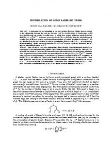
4.2. Conversion of causal bond graphs into block diagrams As a causal bond represents a bi-lateral signal flow with fixed directions, a causal bond graph (e.g. Fig. 2a) can be expanded into a block diagram in three to four steps: all node symbols are encircled and all bonds are expanded into bilateral signal flows according to the assigned causality (Fig. 2b). all constitutive relations of each node are written into block diagram form, according to the assigned causality of each port; zero-junctions are represented by a signal-node for the efforts and a summation for the flows, while one-junctions are represented by a signal-node for the flows and a summation for the efforts(Fig. 2c). all signals entering a summation resulting from a junction are given a sign corresponding to the half-arrow direction: if, while traveling from causal input to causal output, the bond orientation does not change (this does not exclude an orientation opposite to the signal direction!), then a plus sign is added representing a positive contribution to the summation; by contrast if the bond orientation does change, then a minus sign is added representing a negative contribution to the summation (Fig. 2d). In principle, a complete block diagram is obtained at this point. However, its topology is not common due to the location of the conjugate signals. This may be omitted in the next step. Optional: Redraw the block diagram in such a way that the inputs are at the left-hand side and the outputs (observed variables) are at the right-hand side (Fig. 2e) with the integrators in the forward path. The block diagram may be manipulated according to the standard rules for block diagrams as to obtain a canonical form. Port-based Modelling and Control
2-8
Proceedings 5th MATHMOD Vienna, February 2006
Fig. 2a: Causal bond graph
(I.Troch, F.Breitenecker, eds.)
Fig. 2b: Expansion of causal bonds into bilateral signals
Fig. 2c: Expansion of the nodes into operational blocks
Fig. 2d: Addition of signs to the summations
Fig. 2e: Conversion into conventional form The procedure to obtain a signal flow graph is completely analogous to the above procedure as all operations represented by blocks, including the signs of the summations, are combined as much as possible and then written next to an edge, while all summations become nodes, as signal nodes can be distinguished from signal summation points by observing the signal directions (signal node has only one input, summation has only one output).
Port-based Modelling and Control
2-9
Proceedings 5th MATHMOD Vienna, February 2006
(I.Troch, F.Breitenecker, eds.)
4.3. Generation of a set of mixed algebraic and differential equations An arbitrary bond graph with n bonds contains 2n conjugate power variables, 2n ports and 2n corresponding port relations (constitutive relations). If a bond graph is made causal, the order in which the causal strokes are assigned to the bonds can uniquely label the bonds and their corresponding efforts and flows by using the sequence numbers of this process as indices. Next the constitutive relation of each port is written in the form that corresponds to the assigned causality. This results in a mixed set of 2n algebraic and first-order differential equations in an assignment statement form. Note that the differential equations that belong to storage ports in preferred integral causality have a time derivative at the left-hand side of the assignment statements, indicating a ‘postponed’ integration, if it were. During numerical simulation, this integration is performed by the numerical integration method to allow for the next model evaluation step. The switched junctions have the same causal port properties as the regular junctions, but no acausal form of the constitutive relations exists, while it necessarily contains ‘if-then-else’ statements that can only be written after causality has been assigned. The algebraic relations can be used to eliminate all the variables that do not represent the state of a storage port or an input variable, thus resulting in a set of ordinary differential equations (ODE) if all storage ports have preferred causality or in a set of differential and algebraic equations (DAE) if there are dependent storage ports. If the elimination of the algebraic relations is done by hand, the following three intermediate steps are advised: • eliminate all variables that are dependent on the identities of junctions (0, 1) and sources ((M)Se, (M)Sf) • eliminate all variables that are related by the algebraic port relations of all the ports that are not junction ports and not source ports ((M)R(S), (M)TF, (M)GY) • eliminate all variables that are related by the port relations of all the ports that are junction summations (0, 1). • if an algebraic loop is present (active arbitrary causality) choose a variable in this loop to write an implicit algebraic relation and solve symbolically if possible. Otherwise the use of an implicit numerical method is required. • if present and possible, eliminate a differentiated state variable at the right-hand side of the relations symbolically if possible. Otherwise the use of an implicit numerical method is required. For example, the bond graph in Fig. 2a contains 10 bonds, 20 equations and 20 variables of which two are state variables, such that 18 variables have to be eliminated. There are 9 identities (2 source and 3+2+2=7 junction ports), 6 multiplications (2x2 transducer + 2 R) and 3 summations (3 junctions) resulting in the 18 necessary algebraic relations. The final result, assuming linearity of the elements, is df3 1 R n 1 = ( e ( t ) − R1 f3 − n1e7 ) = − 1 f3 − 1 e7 + e ( t ) dt I1 I1 I1 I1
(1)
⎞ ⎞ n1 de7 R2 ⎛ 1 R R 1 ⎛ = f3 − 2 e7 + 2 f ( t ) ⎜ n1 f3 − ⎜ e7 − f ( t ) ⎟ ⎟⎟ = 2 dt C1 ⎜⎝ r1 ⎝ r1 C C C1r1 ⎠⎠ 1 1r1
(2)
⎡ R1 ⎢− I d ⎡ f3 ⎤ ⎢ 1 ⎢ ⎥= dt ⎣ e7 ⎦ ⎢ n1 ⎢ ⎣⎢ C1
(3)
or in matrix form: n ⎤ ⎡ 1 ⎤ − 1 ⎥ ⎢ I1 ⎡ f3 ⎤ I1 ⎥ ⎡ e ( t ) ⎤ ⎥ ⎥ +⎢ ⎢ ⎥ R2 ⎥ ⎣ e7 ⎦ ⎢ R2 ⎥ ⎢⎣ f ( t ) ⎥⎦ − ⎥ ⎢ ⎥ C1r12 ⎦⎥ ⎣ C1r1 ⎦
5. Conclusion The above examples were intended to give a flavor of the content of the first chapter of the Geoplex book. Some of the content of the main text can also be found in the tutorial contribution to the Mathmod in 2003 [6]. 6. [1] [2] [3]
References Paynter, H.M., Analysis and Design of Engineering Systems, MIT Press, 1961. Shearer, J.L., Murphy, A.T., Richardson, H.H., Introduction to System Dynamics, Wesley, NY, 1971. Breedveld, P.C., Thermodynamic Bond Graphs and the problem of thermal inertance, J. Franklin Inst., Vol. 314, No. 1 (1982) 15-40. [4] Breedveld, P.C., Physical Systems Theory in terms of Bond Graphs, ISBN 90-9000599-4, 1984. [5] Maschke, B.M., Schaft, A.J. van der, and Breedveld, P.C., ‘An intrinsic Hamiltonian formulation of dynamics of LC-circuits’, Trans. IEEE on Circuits and Systems, Vol. 42, No. 2, pp. 73-82, Feb. 1995. [6] Breedveld, P.C., Port-Based modeling of mechatronic systems, Mathematics and Computers in Simulation 66, Elsevier, pp. 99 -127, 0378-4754, 2004.
Port-based Modelling and Control
2 - 10