6. External Memory Computational Geometry Revisited

6. External Memory Computational Geometry Revisited Christian Breimann and Jan Vahrenhold∗

6.1 Introduction Computational Geometry is an area in Computer Science basically concerned with the design and analysis of algorithms and data structures for problems involving geometric objects. This field started in the 1970’s and has evolved into a discipline reaching out to areas such as Complexity Theory, Discrete and Combinatorial Geometry, or Algorithm Engineering. Geometric problems occur in a variety of applications, e.g., Computer Graphics, Databases, Geosciences, or Medical Imaging, and there are several textbooks presenting (internal memory) geometric algorithms [239, 275, 342, 541, 566, 596, 614, 647]. The systematic investigation of geometric algorithms specifically designed for massive data sets started in the early 1990’s, most noticeably after Goodrich et al. presented their pioneering paper “External Memory Computational Geometry” [345]. In our survey, we intend to give an overview of results that have been obtained during the last decade and try to relate these results to internal memory algorithms as well. We will review algorithms and data structures for geometric problems involving massive data sets. Our focus will be both on theoretical results and on practical applications. Due to this double focus, this chapter contains not only an overview of fundamental geometric problems and corresponding specialized algorithms and data structures developed in the areas of Computational Geometry and Spatial Databases, but we also discuss how general-purpose index structures already implemented in commercial database systems can be used for solving geometric problems. As a prominent application area involving massive data sets, spatial database systems have attracted increasing interest both in research communities and among professional users. In addition to the growing number of applications, the increasing availability of spatial data in form of digital maps and images is one of the main reasons for this trend, and tightly coupled to this, applications demand sophisticated computations and complex analyses of such data. In this area, it is not uncommon to use sub-optimal algorithms (in terms of their asymptotic complexity) if they lead to better performance in practice. ∗

Part of this work was done while on leave at the University for Health Informatics and Technology Tyrol, 6020 Innsbruck, Austria.

U. Meyer et al. (Eds.): Algorithms for Memory Hierarchies, LNCS 2625, pp. 110-148, 2003.  Springer-Verlag Berlin Heidelberg 2003

6. External Memory Computational Geometry Revisited

111

The geometric problems described in the remainder of this survey are grouped according to the kind of objects for which the problem is defined. In Section 6.3, we describe problems involving sets of points (Problems 6.1– 6.11), in Section 6.4, we present a discussion of problems involving sets of segments (Problems 6.12–6.20), and in Section 6.5, we conclude by surveying problems involving sets of polygons (Problem 6.21 and Problem 6.22). Table 6.1 contains an overview of all problems covered in this chapter. Table 6.1. Geometric problems surveyed in this chapter. No.

Problem name

No.

1 2 3 4 5 6 7 8

Convex Hull Halfspace Intersection Closest Pair K-Bichromatic Closest Pairs Nearest Neighbor All Nearest Neighbors Reverse Nearest Neighbors K-Nearest Neighbors

12 13 14 15 16 17 18 19

9 10 11

Halfspace Range Searching Orthogonal Range Searching Voronoi Diagram

20 21 22

Problem Name Segment Stabbing Segment Sorting Endpoint Dominance Trapezoidal Decomposition Polygon Triangulation Vertical Ray-Shooting Planar Point Location Bichromatic Segment Intersection Segment Intersection Rectangle Intersection Polygon Intersection

Whenever appropriate, we will sub-classify problems according to the extent to which the sets may be updated: Static Setting: All data items are fixed prior to running an algorithm or building a data structure, and no changes to the data items may occur afterwards. Dynamic Setting: The set of items that forms the problem instance can be updated by insertions as well as deletions. Semidynamic Setting: The set of items that forms the problem instance can be updated by either insertions or deletions, but not both. The dynamic and semidynamic setting can also be considered in a batched variant, that is, all updates have to be known in advance. For problems that involve answering queries, we additionally distinguish between two kinds of queries: Single-Shot Queries: Each query has to be answered independent of other queries and before the next query may be posed. Batched Queries: The user specifies a collection of queries, and the only requirement is that all queries are answered by the end of the algorithm.

112

Christian Breimann and Jan Vahrenhold

Before surveying geometric problems and corresponding solutions, we will briefly review the model of computation and introduce three general techniques for solving large-scale geometric problems.

6.2 General Methods for Solving Geometric Problems External memory algorithms are investigated analytically in the parallel disk model introduced by Aggarwal and Vitter [17] and later refined by Vitter and Shriver [755]. The parallel disk model, which is based on blocked transfers, uses the following parameters: N M B D P

= = = = =

Number Number Number Number Number

of of of of of

objects in the problem instance objects that fit simultaneously into main memory objects that fit into one disk block independent disks parallel processors

In this survey, however, we will restrict ourselves to algorithms for singledisk/single-processor settings, that is, we assume D = 1 and P = 1. For algorithms involving multiple queries, we consider two additional parameters: Q Z

= =

Number of queries Number of objects in the answer set

This model allows computations only on elements that are in main memory, and whenever additional elements are needed in main memory, they have to be read from disk. The measures of performance for an external memory algorithm are the number of I/Os performed during its execution and the amount of disk space occupied (in terms of disk blocks). In the remainder of this section, we present some general methods which are often used to solve geometric problems. First of all, we briefly discuss the implications of solving a problem by reducing it to a problem for which an efficient algorithm is known and present the concept of duality which sometimes can be used for this purpose (Section 6.2.1). In Section 6.2.2, we describe the general distribution sweeping paradigm, an external version of the well-known plane sweeping. Section 6.2.3 covers the R-tree, a spatial index structure frequently used in spatial database systems, and some of its variants. 6.2.1 Reduction of Problems A common technique for proving lower bounds for (geometric) problems is to reduce the problem to some fundamental problem for which a lower bound is known. Among these fundamental problems is the Element Uniqueness problem which is, given a collection of N objects, to determine whether any two


113

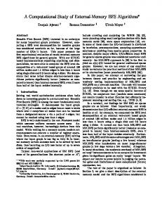
are identical. The lower bound for this problem is Ω((N/B) logM/B (N/B)) [59], and—looking at the reduction from the opposite direction—a matching upper bound for the Element Uniqueness problem for points can be obtained by solving what is called the Closest Pair problem (see Problem 6.3). For a given collection of points, this problem consists of computing a pair with minimal distance. This distance is non-zero if and only if the collection does not contain duplicates, that is if and only if the answer to the Element Uniqueness problem is negative.

(a) Concept of transformation.

(b) Transformation of bounds.

Fig. 6.1. Reduction of problems.

A more general view is given by Figure 6.1. It shows that reducing (transforming) a problem A to a problem B means transforming the input of A first, then solving problem B, and transforming its solution back afterwards (see Figure 6.1 (a)). Such a transformation is said to be a τ (N )-transformation if and only if transforming both the input and the solution can be done in O(τ (N )) time. If an algorithm for solving the problem B has an asymptotic complexity of O(fB (N )), the problem A can be solved in O(fB (N ) + τ (N )) time. In addition, if the intrinsic complexity of the problem A is Ω(fA (N )) and if τ (N ) ∈ o(fA (N )), then B also has a lower bound of Ω(fA (N )) (see Figure 6.1 (b) and, e.g., the textbook by Preparata and Shamos [614, Chap. 1.4]). Reduction via Duality In Section 6.3, which is entitled “Problems Involving Sets of Points”, we will discuss the following problem (Problem 6.2): “Given a set S of N halfspaces in IRd , compute the common intersection of these halfspaces.” At first, it seems surprising that this problem should be discussed in a section devoted to problems involving set of points. Using the concept of geometric duality, however, points and halfspaces can be identified in a consistent way: A duality transform maps points in IRd into the set G d of non-vertical hyperplanes in IRd and vice versa. The classical duality transform between points and hyperplanes is defined as follows: D:

d−1 G d → IRd : xd = ad + i=1 ai xi → (a1 , . . . , ad ) d−1 IRd → G d : (b1 , . . . , bd ) → xd = bd − i=1 bi xi

114


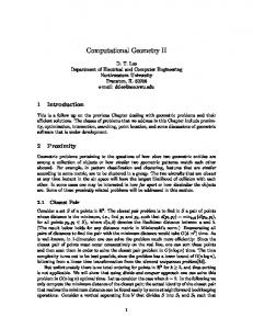
Another well-known transform D that is used, e.g., in the context of the Convex Hull problem (Problem 6.1), maps a point p on the unit parabola to the unique hyperplane that is tangent to the parabola in p. For the sake of simplicity, this duality transform is stated for d = 2. 2 G → IR2 : y = 2ax − b → (a, b) D: IR2 → G 2 : (a, b) → y = 2ax − b An important property of these transforms is that they are their own inverses and that they preserve the “above-below” relation: a point p lies above (below) the hyperplane with respect to the d-th dimension if and only if the line D(p) lies above (below) the point D() with respect to the d-th dimension. This property is exploited in several algorithms for, e.g., the Range Searching problem, the Convex Hull problem, the K-Nearest Neighbors problem, or the Voronoi Diagram problem. These algorithms first reduce the original problem to a problem stated for the duals of the original objects, solve the problem in the dual setting, and finally employ the same duality transform to obtain the solution to the original problem. We refer the interested reader to textbooks on Computational Geometry (e.g. [275, 541, 596]) for a more detailed treatment of these duality transforms. 6.2.2 Distribution Sweeping A large number of internal memory algorithms is based upon plane sweeping, a general technique for turning a static (d + 1)-dimensional problem into a (finite) collection of instances of a dynamic d-dimensional problem. Although the general approach is independent of the dimension d, it is most efficient when the (original) problem is two-dimensional, and therefore we will restrict the following description to this setting. The characterizing feature of the plane sweeping technique is an (imaginary) line (or, in the general setting, a hyperplane) that is swept over the entire data set. For sake of simplicity, this sweep-line is usually assumed to be perpendicular to the x-axis of the coordinate system and to move from left to right. Any object intersected by the sweep-line at x = t is called active at time t, and only active objects are involved in geometric computations at that time. In the situation depicted in Figure 6.2(a), the sweep-line is drawn in bold, and the active objects, i.e., the objects intersected by the sweep-line, are the line segments A and B. To guarantee the correctness of a plane-sweep algorithm, one has to take care of restating the original problem in such a way that operations involving only active objects are sufficient to determine the proper solution to the problem, e.g., Graf [350] summarized several formulations of plane-sweep algorithms. All objects active at a given time are usually stored in a dictionary called sweep-line structure. The status of the sweep-line structure is updated as soon


(a) Internal plane sweeping.

115

(b) External distribution sweeping.

Fig. 6.2. The plane sweeping and distribution sweeping techniques.

as the sweep-line moves to a point where the topology of the active objects changes discontinuously: for example, an object must be inserted into the sweep-line structure as soon as the sweep-line hits its leftmost point, and it must be removed after the sweep-line has passed its rightmost point. The sweep-line structure can be maintained in logarithmic time per update if the objects can be ordered linearly, e.g., by the y-value of their intersection with the sweep line. For a finite set of objects, there are only finitely many points where the topology of the active objects changes discontinuously, e.g., when objects are inserted into or deleted from the sweep-line structure; these points are called events and are stored in increasing order of their x-coordinates, e.g, in a priority queue. Depending on the problem to be solved, there may exist additional event types apart from insert and delete events. The data structure for storing the events is called event queue, and maintaining it as a priority queue under insertions and deletions can be accomplished in logarithmic time per update. That is, if the active objects can be ordered linearly, each event can be processed in logarithmic time (excluding the time needed for operations involving active objects). As a consequence, the plane sweeping technique often leads to optimal algorithms, e.g., the Closest Pair problem can be solved in optimal time O(N log2 N ) [398]. The straightforward approach for externalizing the plane sweeping technique would be to replace the (internal) sweep-line structure by a corresponding external data structure, e.g., a B-tree [96]. A plane-sweep algorithm with an internal memory time complexity of O(N log2 N ) then spends O(N logB N ) I/Os. For problems with an external memory lower bound of Ω((N/B) logM/B (N/B)), however, the latter bound is at least a factor of B away from optimal.1 The key to an efficient external sweeping technique is to combine sweeping with ideas similar to divide-and-conquer, that is, to subdivide the plane prior to sweeping. To aid imagination, consider the plane subdivided into Θ(M/B) parallel (vertical) strips, each containing the same 1

Often the (realistic) assumption M/B > B is made. In such a situation, an additional (non-trivial) factor of logB M > 2 is lost.

116


number of data objects (see Figure 6.2(b)).2 Each of these strips is then processed using a sweep over the data and eventually by recursion. However, in contrast to the description of the internal case, the sweep-line is perpendicular to the y-axis, and sweeping is done from top to bottom. The motivation behind this modified description is to facilitate the intuition behind the novel ingredient of distribution sweeping, namely the subdivision into vertical strips. The subdivision proceeds using a technique originally proposed for distribution sort [17], hence, the resulting external plane sweeping technique has been christened distribution sweeping [345]. While in the situation of distribution sort all partitioning elements have to be selected using an external variant of the median find algorithm [133, 307], distribution sweeping can resort to having an optimal external sorting algorithm at hand. The set of all x-coordinates is sorted in ascending order, and for each (recursive) subdivision of a strip, the Θ(M/B) partitioning elements can be selected from the sorted sequence spending an overall number of O(N/B) I/Os per level of recursion. Using this linear partitioning algorithm as a subroutine, the distribution sweeping technique can be stated as follows: Prior to entering the recursive procedure, all objects are sorted with respect to the sweeping direction, and the set of x-coordinates is sorted such that the partitioning elements can be found efficiently. During each recursive call, the current data set is partitioned into M/B strips. Objects that interact with objects from other strips are found and processed during a sweep over the strips, while interactions between objects assigned to the same strip are found recursively. The recursion terminates when the number of objects assigned to a strip falls below M and the subproblem can be solved in main memory. If the sweep for finding inter-strip interactions can be performed using only a linear number of I/Os, i.e., Θ(N/B) I/Os, the overall I/O complexity for distribution sweeping is O((N/B) logM/B (N/B)). 6.2.3 The R-tree Spatial Index Structure Many algorithms proposed in the context of spatial databases assume that the data set is indexed by a hierarchy of bounding boxes. This assumption is justified by the popularity of the R-tree spatial index structure (and its variants) in academic and commercial database systems. The R-tree, originally proposed by Guttman [368], is a height-balanced multiway tree similar to a B-tree. An R-tree stores d-dimensional data objects approximated by their axis-parallel minimum bounding boxes. For ease of 2

Non-point objects cannot always be assigned to a unique strip because they may interact with several strips. In such a situation, objects are assigned to a maximal contiguous interval of strips they interact with. See the discussion of, e.g., Problem 6.20 for more details on how to deal with such a situation.


117

presentation, we restrict the following discussion to the situation d = 2 and assume that each data object itself is an axis-parallel rectangle. The leaf nodes in an R-tree contain Θ(B) data rectangles each, where B is the maximum fanout of the tree. Internal nodes contain Θ(B) entries of the form (Ptr ,R), where Ptr is a pointer to a child node and R the minimum bounding rectangle covering all rectangles which are stored in the subtree rooted in that child. Each entry in a leaf stores a data object or, in the general setting, the bounding rectangle of a data object and a pointer to the data object itself. Since the bounding rectangles stored within internal nodes are used to guide the insertion, deletion, and querying processes (see below), they are referred to as routing rectangles, whereas the bounding rectangles stored in the leaves are called data rectangles. An R-tree for N rectangles consists of O(N/B) nodes and has height O(logB N ). Figure 6.3 shows an example of an R-tree for a set of two-dimensional rectangles.

Fig. 6.3. R-tree for data rectangles A, B, C, . . . , I, K, L. The tree in this example has maximum fanout B = 3.

To insert a new rectangle r into an already existing R-tree with root v, we select the subtree rooted at v whose bounding rectangle needs least enlargement to include the new rectangle. The insertion process continues recursively until a leaf is reached, adjusting routing rectangles as necessary. Since recursion takes place along a single root-to-leaf path, an insertion can be performed touching only O(logB N ) nodes. If a leaf overflows due to an insertion, a rebalancing process similar to B-tree rebalancing is triggered, and therefore R-trees also grow and shrink only at the root. The insertion path depends not only on the heuristic chosen for breaking ties in case of non-unique subtrees for recursion, but also on the objects already present in the R-tree. Hence, there is no unique R-tree for a given set of rectangles, and different orders of insertion for the same set of rectangles usually result in different R-trees. During the insertion process, a new rectangle r might overlap the routing rectangles of several subtrees of the node v currently visited. However, the rectangle r is routed to exactly one such subtree. Since the routing rectangle

118


of this subtree might be extended to include r, the routing rectangles stored within v can overlap. This overlap directly affects the performance of R-tree query operations: When querying an R-tree to find all rectangles overlapping a given query rectangle r, we have to branch at each internal node into all subtrees whose minimum bounding rectangle overlaps r. (Queries for all rectangles containing a given query point p can be stated in the same way by regarding p as an infinitesimally small rectangle.) In the worst case, the search process has to branch at each internal node into all subtrees which results in O(N/B) nodes being touched—even though the number of reported overlapping data rectangles might be much smaller. Intuitively, it is thus desirable that the routing rectangles stored within a node overlap as little as possible. Another heuristic is to minimize the area covered by each routing rectangle. As a consequence routing rectangles cover less dead space, i. e., space covered by a routing rectangle which is not covered by any child, such that unsuccessful searches may terminate earlier. Similar heuristics are used in several variants of the R-tree including the R+ -tree [683], the Hilbert Rtree [442], and the R* -tree [102], which is widely recognized to be the most practical R-tree variant. This is especially due to the fact that the heuristics used in the R* -tree re-insert a certain number of elements if routing rectangles have to be split. This usually results in a re-structured tree with less overlapping of routing rectangles permitting fast answers for queries. We refer the interested reader also to the Generalized Search Tree [50, 389] and to more detailed overviews [323, 754]. As mentioned above, overlapping routing rectangles decrease the query performance of R-trees, and with increasing dimension, this overlap grows rapidly. Therefore, other data structures, e.g., the X-tree [114], which uses so-called supernodes permitting a sequential scan of their children, have been developed. But as the percentage of the data space covered by routing rectangles grows quickly with increasing dimensionality, for d > 10, nearly every node is accessed when querying the data structure as long as nodes are split in a balanced way. For many data distributions, a sequential scan can have better query performance in terms of overall running time than the random I/Os caused by querying data structures which are based on datapartitioning [758]. With the Pyramid-Technique [113], points and ranges in d-dimensional data space are transformed to 1-dimensional values which can be stored and queried using any 1-dimensional data structure, e.g., a B+ -tree. The authors claim that the Pyramid-Technique using a B+ -tree outperforms not only the data structures presented above but also the sequential scan. We have presented some hierarchical spatial index structures which are used to efficiently store and query multi-dimensional data objects. From now on, whenever we refer to a hierarchical spatial index structure, any of these structures may be used unless explicitly stated otherwise.


119

6.3 Problems Involving Sets of Points The first problem we discuss in this section is not only one of the most fundamental problems studied in Computational Geometry but also one of the rare problems where finding an optimal external algorithm for the twodimensional case is completely straightforward.

(a) Planar convex hull.

(b) Intersection of halfspaces in dual space.

Fig. 6.4. Computing the convex hull of a finite point set.

Problem 6.1 (Convex Hull). Given a set S of N points in IRd , find the smallest (convex) polytope enclosing S (see Figure 6.4(a)). Among the earliest internal memory algorithms for computing the convex hull in two dimensions was a sort-and-scan algorithm due to Graham [352]. This algorithm, called Graham’s Scan, is based upon the invariant that when traversing the boundary of a convex polygon in counterclockwise direction, any three consecutive points form a left turn. The algorithm first selects a point p that is known to be interior to the convex hull, e.g., the center of gravity of the triangle formed by three non-collinear points in S. All points in S are then sorted by increasing polar angle with respect to p. The convex hull is constructed by pushing the points onto a stack in sorted order, maintaining the above invariant. As soon as the next point to be pushed and the topmost two points on the stack do not form a left turn, points are repeatedly removed from the stack until only one point is left or the invariant is fulfilled. After all points have been processed, the stack contains the points lying on the convex hull in clockwise direction. As each point can be pushed onto (removed from) the stack only once, Θ(N ) stack operations are performed, and the (optimal) internal memory complexity, dominated by the sorting step, is O(N log2 N ). This algorithm is one of the rare cases where externalization is completely straightforward [345]. Sorting can be done using O((N/B) logM/B (N/B)) I/Os [17], and an external stack can be implemented such that Θ(N ) stack operations require O(N/B) I/Os (see Chapter 2). The external algorithm we obtain this way has an optimal complexity of O((N/B) logM/B (N/B)). In general, O(N ) points of S can lie on the convex hull, but there are situations where the number Z of points on the convex hull is (asymptotically) much smaller. An output-sensitive algorithm for computing the convex hull

120


in two dimensions has been obtained by Goodrich et al. [345]. Building upon the concept of marriage-before-conquest [458], the authors combine external versions of finding the median of an unsorted set [17] and of computing the convex hull of a partially sorted point set [343] to obtain an optimal outputsensitive external algorithm with complexity O((N/B) logM/B (Z/B)). Independent from this particular problem, Hoel and Samet [402] claimed that accessing disjoint decompositions of data space tends to be faster than other decompositions for a wide range of hierarchical spatial index structures. Along these lines, B¨ ohm and Kriegel [138] presented two algorithms for solving the Convex Hull problem using spatial index structures. One algorithm, computing the minimum and maximum values for each dimension and traversing the index depth-first, is shown to be optimal in the number of disk accesses as it reads only the pages containing points not enclosed by the convex hull once. The second algorithm performs worse in terms of I/O but needs less CPU time. It is unclear, however, how to extend these algorithms to higher dimensions. An approach to the d-dimensional Convex Hull problem is based on the observation that the convex hull of S ⊂ IRd can be inferred from the intersection of halfspaces in the dual space (IRd )∗ [781] (see also Figures 6.4(a) and (b)). For each point p ∈ S, the corresponding dual halfspace is given by p∗ := {x ∈ (IRd )∗ | di=1 xi pi ≤ 1}. At least for d ∈ {2, 3}, the intersection of halfspaces can be computed I/O-efficiently (see the following Problem 6.2), and this results in corresponding I/O-efficient algorithms for the Convex Hull problem in these dimensions. Problem 6.2 (Halfspace Intersection). Given a set S of N halfspaces in IRd , compute the common intersection of these halfspaces. In the context of the Halfspace Intersection problem, efficient external algorithms are known only for the situation d ≤ 3. The intersection in three dimensions can be computed by either using an externalization of Reif and Sen’s parallel algorithm [630] (as proposed by Goodrich et al. [345]) or by an algorithm that can be derived in the framework of randomized incremental construction with gradations [228] (see Section 6.4). Both algorithms require O((N/B) logM/B (N/B)) I/Os (for the first approach, this bound holds with high probability, while it is the expected complexity for the second approach). The problem we discuss next has already been mentioned in the context of solving problems by reduction (Section 6.2.1): Problem 6.3 (Closest Pair). Given a set S of N points in IRd and a distance metric d, find a pair (p, q) ∈ S × S, p = q, for which d(p, q) = min{d(r, s) | r, s ∈ S, r = s} (see Figure 6.5(a)). There is a variety of optimal algorithms in the internal memory setting that solve the problem either directly or by exploiting reductions to other


(a) Closest pair.

121

(b) Nearest neighbor for query point p.

Fig. 6.5. Closest-point problems.

problems (see also the survey by Smid [700]). In the external memory setting, the (static) problem of finding the closest pair in a fixed set S of N points can be solved by exploiting the reduction to the All Nearest Neighbors problem (Problem 6.6), where for each point p ∈ S, we wish to determine its nearest neighbor in S \ {p} (see Problem 6.5). Having computed this list of N pairs of points, we can easily select two points forming a closest pair by scanning the list while keeping track of the closest pair seen so far. As we will discuss below, the complexity of solving the All Nearest Neighbors is O((N/B) logM/B (N/B)), which gives us an optimal algorithm for solving the static Closest Pair problem. Handling the dynamic case is considerably more involved, as an insertion or a deletion could change a large number of “nearest neighbors”, and consequently, the reduction to the All Nearest Neighbors problem would require touching at least the same number of objects. Callahan, Goodrich, and Ramaiyer [168] introduced an external variant of topology trees [316], and building upon this data structure, they managed to develop an external version of the dynamic closest pair algorithm by Bespamyatnikh [121]. The data structure presented by Callahan et al. can be used to dynamically maintain the closest pair spending O(logB N ) I/Os per update. The Closest Pair problem can also be considered in a bichromatic setting, where each point is labeled with either of two colors, and where we wish to report a pair with minimal distance among all pairs of points having different colors [10, 351]. This problem can be generalized to the case of reporting the K bichromatic closest pairs. Problem 6.4 (K-Bichromatic Closest Pairs). Given a set S of N points in IRd with S = S1 ∪ S2 and S1 ∩ S2 = ∅, find K closest pairs (p, q) ∈ S1 × S2 . Some efficient internal memory algorithms for solving this problem have been proposed [10, 451], but it seems that none of them can be externalized efficiently. In the context of spatial databases, the K-Bichromatic Closest Pairs problem can be seen as a special instance of a so-called θ-join which is defined as follows: Given two sets S1 and S2 of objects and a predicate θ : S1 × S2 → IB, compute all pairs (s1 , s2 ) ∈ S1 × S2 , for which θ(s1 , s2 ) = true. In his approach to the K-Bichromatic Closest Pairs problem,Henrich [393] considered the special case |S2 | = 1, and assuming that S1 is indexed hier-

122


archically, he proposed to perform a priority-driven traversal of the spatial index structure storing S1 . Hjaltason and Samet [401] later generalized this approach and referred to Problem 6.4 as a special instance of a θ-join, namely the incremental distance join (again assuming that each relation is indexed hierarchically). Their algorithm schedules a priority-driven synchronous traversal of both trees, repeatedly looking at two nodes, one from each tree. The processing is guided by the distance between the (routing) rectangles corresponding to the nodes, and to each pair this distance is assigned as the pair’s priority. Initially, the priority queue contains all pairs that can be formed by grouping the root of one tree and the children of the root of the other tree, and the first element in the queue always forms the closest pair of objects stored in the queue. For each removed pair of nodes, the pairs formed by the children (if any) are inserted into the queue. Whenever a pair of data objects appears at the front of the queue, its associated distance is minimal among all unconsidered distances, hence, all K bichromatic closest pairs can be reported ordered by increasing distance. This algorithm benefits from the observation that in practical applications K |S1 ×S2 |, but nevertheless, the priority queue might contain a large number of pairs. Hjaltason and Samet described several approaches for how to organize the priority queue such that only a small portion of it actually resides in main memory. This means that only the promising candidate pairs are kept in main memory whereas all pairs having a large distance are off-loaded to external memory. The authors argue that except for unlikely worst-case configurations, their approaches perform without accessing the off-loaded data and that worst-case configurations can be handled gracefully as well. Worst-case optimal external priority queues are also discussed in Chapter 2 and Chapter 3. Corral et al. [219] presented a collection of algorithms that improve the effective running time of the above algorithms for solving the Bichromatic Closest Pair problem. These improvements include a separate treatment for the case K = 1 and choosing a heap-based priority queue. These algorithms for solving Problem 6.4 can be modified to solve (the monochromatic) Problem 6.3. This modification is not generally possible [219] for an arbitrary algorithm solving Problem 6.4. A description of modifications for the latter algorithm has been given by Corral et al. [218]. The authors claim that these modifications do not seriously affect the performance of their algorithm. As mentioned before, spatial index structures try to cluster objects based upon their spatial location, and consequently, several approaches have been made to exploit this structural property when dealing with proximity problems. A fundamental proximity problem is to organize a set of points such that for each query point the point closest to it can be reported quickly. Problem 6.5 (Nearest Neighbor). Given a set S of N points in IRd , a distance metric d, and a query point p in IRd , report a point q ∈ S, for which d(p, q) = min{d(p, r) | r ∈ S} (see Figure 6.5(b)).


123

Problem 6.5 and its relatives occur in a variety of conventional geographical applications, e.g., when searching for the closest geometric feature of some kind relative to some given spatial location. This problem is also referred to as the Post Office problem [460]3 . Since the metric d defining the “closeness” of two objects is also a parameter in the problem setting, this problem can be found in new application areas like multimedia database systems. In this setting, multimedia objects, e.g., text, image, or video objects, are described by high-dimensional feature vectors which in turn are considered as points in the feature space. Proximity among these feature vectors implies similarity between the objects represented, and in combination with carefully chosen metrics, spatial index structures can be used for efficiently performing similarity search [137, 473, 668, 681]. The Nearest Neighbor problem can also be restated in the context of Voronoi diagrams (see Problem 6.11), and using techniques by Goodrich et al. [345], one can obtain a static data structure that answers nearest neighbor queries in O(logB N ) I/Os. We will comment on this approach when discussing algorithms for computing the Voronoi diagram.

(a) Approximate nearest neighbor.

(b) All nearest neighbors.

Fig. 6.6. Nearest-neighbor problems.

A variant of the Nearest Neighbor problem is to compute an approximate nearest neighbor for a given query point. Here, an additional parameter ε is used to allow for certain slack in the reported “minimum” distance. For ε > 0, a (1 + ε)-approximate nearest neighbor of a query point p is a point q that is no further than (1 + ε) times the distance dist to the actual nearest neighbor of p (see Figure 6.6(a)). Using external topology trees, Callahan et al. [168] derived an external version of the data structure by Arya et al. [72] that can be used to maintain S under insertions and deletions with O(logB N ) I/Os per update such that an approximate nearest neighbor query can be answered spending O(logB N ) I/Os.4 Even in the internal memory setting, it is an open problem to find an efficient dynamic data structure with O(N logO(1) N ) space that can be used for the exact Nearest Neighbor problem and has O(logO(1) N ) update 3

4

This reference is ascribed to Knuth as he discusses a data structure called postoffice tree which can be used for answering a query of the kind “What is the nearest city to point x?”, given the value of x [460, page 563]. The constants hidden in the “Big-Oh”-notation depend on d and ε.

124


and query time [700], and not surprisingly, the external memory variant of this problem is unsolved as well. Berchtold et al. [112] proposed to use hierarchical spatial index structures to store the data points. They also introduced a different cost model and compared the predicted and actual cost of solving the Nearest Neighbor problem for real-world data using an X-tree [114] and a Hilbert-R-tree [287]. Brin [148] introduced the GNAT index structure which resembles a hierarchical Voronoi diagram (see Problem 6.11). He also gave empirical evidence that this structure outperforms most other index structures for high-dimensional data spaces. The practical relevance of the nearest neighbor, however, becomes less significant as the number of dimensions increases. For both real-world and synthetic data sets in high-dimensional space (d > 10), Weber, Schek, and Blott [759] as well as Beyer et al. [123] showed that under several distance metrics the distance to the nearest neighbor is larger than the distance between the nearest neighbor and the farthest neighbor of the query point. Their observation raises an additional quality issue: The exact nearest neighbor of a query point might not be relevant at all. As an approach to cope with this complication, Hinneburg, Aggarwal, and Keim [397] modified the Nearest Neighbor problem by introducing the notion of important dimensions. They introduced a quality criterion to determine which dimensions are relevant to the specific proximity problem in question and examined the data distribution resulting from projections of the data set to these dimensions. Obviously, their approach yields improvements over standard techniques only if the number of “important” dimensions is significantly smaller than the dimension of the data space. Problem 6.6 (All Nearest Neighbors). Given a set S of N points in IRd and a distance metric d, report for each point p ∈ S a point q ∈ S, for which d(p, q) = min{d(p, r) | r ∈ S, p = r} (see Figure 6.6(b)). The All Nearest Neighbors problem, which can also be seen as a special batched variant of the (single-shot) Nearest Neighbor problem, can be posed, e.g., in order to find clusters within a point set. Goodrich et al. [345] proposed an algorithm with O((N/B) logM/B (N/B)) I/O-complexity based on the distribution sweeping paradigm: Their approach is to externalize a parallel algorithm by Atallah and Tsay [74] replacing work on each processor by work within a single memory load. Recall that on each level of distribution sweeping, only interactions between strips are handled, and that interactions within a strip are handled recursively. In the situation of finding nearest neighbors, the algorithm performs a top-down sweep keeping track of each point whose nearest neighbor above does not lie within the same strip. The crucial observation by Atallah and Tsay is that there are at most four such points in each strip, and by choosing the branching factor of distribution sweeping as M/(5B), the (at most) four blocks per strip containing these


125

points as well as the M/(5B) blocks needed to produce the input for the recursive steps can be kept in main memory. Nearest neighbors within the same strip are found recursively, and the result is combined with the result of a second bottom-up sweep to produce the final answer. In several applications, it it desirable to compute not only the exact nearest neighbors but to additionally compute for each point the K points closest to it. An algorithm for this so-called All K-Nearest Neighbors problem has been presented by Govindarajan et al. [346]. Their approach (which works for an arbitrary number d of dimensions) builds upon an external data structure to efficiently maintain a well-separated pair decomposition [169]. A well-separated pair decomposition a set S of points is a hierarchical clustering of S such that any two clusters on the same level of the hierarchy are farther apart than any to points within the same cluster, and several internal memory algorithms have been developed building upon properties of such a decomposition. The external data structure of Govindarajan et al. occupies O(KN/B) disk blocks and can be used to compute all K-nearest neighbors in O((KN/B) logM/B (KN/B)) I/Os. Their method can also be used to compute the K closest pairs in d dimensions in O(((N + K)/B) logM/B ((N + K)/B)) I/Os using O((N + K)/B) disk blocks.

(a) Reverse nearest neighbors for point p.

(b) K-nearest neighbors via lifting.

Fig. 6.7. Non-standard nearest-neighbor problems.

Problem 6.7 (Reverse Nearest Neighbors). Given a set S of N points in IRd , a distance metric d, and a query point p in IRd , report all points q ∈ S, for which d(q, p) = min{d(q, r) | r ∈ (S ∪ {p}) \ {q}} (see Figure 6.7(a)). The Reverse Nearest Neighbors problem has been introduced in the spatial database setting by Korn and Muthukrishnan [472] who also presented static and dynamic solutions for the bichromatic an monochromatic problem. For simplicity, we only discuss the solution to the static monochromatic problem here, as for their approach only minor modifications are needed to solve the other three problems. In a preprocessing step, the All Nearest Neighbors problem is solved for S. Each point q and its nearest neighbor r define a ball centered at q with radius d(q, r). All N such balls are stored in a spatial index structure that can be used to report, given a query point p, all balls

126


containing p. It is easy to verify that the points corresponding to the balls that contain p are exactly the points having p as their nearest neighbor in S ∪ {p}. In the internal memory setting, at least the static version of the Reverse Nearest Neighbor problem can be solved efficiently [524]. The main problem when trying to efficiently solve the problem in a dynamic setting is that updating S essentially involves finding nearest neighbors in a dynamically changing point set, and—as discussed in the context of Problem 6.5—no efficient solution with at most polylogarithmic space overhead is known. Problem 6.8 (K-Nearest Neighbors). Given a set S of N points in IRd , an integer K with 1 ≤ K ≤ N , and a query point p in IRd , report K points qi ∈ S closest to p. Agarwal et al. [6] solved the two-dimensional K-Nearest Neighbors problem in the dual setting: using a duality transform, they proposed to map each two-dimensional point (a1 , a2 ) to the hyperplane z = a21 + a22 − 2a1 x − 2a2 y which is tangent to the unit parabola at the (lifted) point (a1 , a2 , a21 + a22 ). In this setting, the problem of finding the K nearest neighbors for a point p = (xp , yp ) can be restated as finding the K highest hyperplanes above the point (xp , yp , 0) (For the sake of simplicity, the corresponding one-dimensional problem is sketched in Figure 6.7(b). Consider, e.g., point O: The two highest hyperplanes lying above O are defined by lifting points B and C which are also the two nearest neighbors of O). Using an external version of Chan’s algorithm for computing (≤ k)-levels of an arrangement [175], Agarwal et al. [6] developed a data structure for range searching among halfplanes that, after spending O((N/B) log2 N logB N ) expected I/Os for preprocessing, occupies an expected number of O((N/B) log2 (N/B)) disk blocks. This data structure can be used to report the K highest halfplanes above a query point, and by duality, the K nearest neighbors in the original setting, spending O(logB N + K/B) expected I/Os per query. In addition to the quite involved data structure mentioned above, spatial index structures have been considered to solve the K-Nearest Neighbor problem [190, 473, 640, 681]. Much attention has been paid to pruning parts of the candidate set [681] and to removing inefficient heuristics [190]. As mentioned above, the performance of most index structures degrades for high dimensions, and even while the Pyramid-Technique [113] can be used for uniformly distributed data in high dimensions, its performance degrades for non-uniformly distributed data. To overcome this deficiency, Yu et al. [774] presented a new approach called iDistance which is adaptable with respect to data distribution. They propose to partition the data space according to its characteristics and, for each partition, to index the distance between contained data points and a reference point using a B+ -tree. Their algorithm can be used to incrementally refine approximate answers such that early during the algorithm, approximate results can be output if desired. In contrast, the VA-file of Weber et al. [758, 759] uses approximated data to produce a


127

set of candidate pairs during nearest neighbor search. It partitions the data space into cells and stores unique bit strings for these cells in an (optionally compressed) array. During a sequential scan of this array, candidates are determined by using the stored approximations, before these candidates are further examined to obtain the final result. Establishing a trade-off between used disk space and obtained query time, Goldstein and Ranakrishnan [338] presented an approach to reduce query time by examining some characteristics of the data and storing redundant information. Following their approach the user can explicitly relate query performance and disk space, i.e., more redundant information can be stored to improve query performance and vice versa. With a small percentage of only approximately correct answers in the final result, this approach leads to sub-linear query processing for high dimensions. The description of algorithms for the K-Nearest Neighbors problem concludes our discussion of proximity problems, that is of selecting certain points according to their proximity to one or more query points. The next two problems also consist of selecting a subset of the original data, namely the set contained in a given query range. These problems, however, have been discussed in detail by recent surveys [11, 56, 754], so we only sketch the main results in this area.

(a) Halfspace range searching.

(b) Orthogonal range searching.

Fig. 6.8. Range searching problems.

Problem 6.9 (Halfspace Range Searching). Given a set S of N points d in IR and a vector a ∈ IRd , report all Z points x ∈ S, for which xd ≤ d−1 ad + i=1 ai xi . The main source for solutions to the halfspace range searching problem in the external memory setting is the paper by Agarwal et al. [6]. The authors presented a variety of data structures that can be used for halfspace range searching classifying their solutions in linear and non-linear space data structures. All proposed algorithms rely on the following duality transform and the fact that it preserves the “above-below” relation. D:

d−1 G d → IRd : xd = ad + i=1 ai xi → (a1 , . . . , ad ) d−1 IRd → G d : (b1 , . . . , bd ) → xd = bd − i=1 bi xi

128


In the linear space setting, the general problem for d > 3 can be solved using an external version of a partition tree [535] spending for any fixed ε > 0 O((N/B)1−1/d+ε + Z/B) I/Os per query. The expected preprocessing complexity is O(N log2 N ) I/Os. For simplex range searching queries, that is for reporting all points in S lying inside a given query simplex with µ faces of all dimensions, O((µN/B)1−1/d+ε +Z/B) I/Os are sufficient. For halfspace range searching and d = 2, the query cost can be reduced to O(logB N +Z/B) I/Os (using O(N log2 N logB N ) expected I/Os to preprocess an external version of a data structure by Chazelle, Guibas, and Lee [184]). Using partial rebuilding, points can also be inserted into/removed from S spending amortized O(log2 (N/B) logB N ) I/Os per update. If one is willing to spend slightly super-linear space, the query cost in the three-dimensional setting can be reduced to O(logB N +Z/B) I/Os at the expense of an expected overall space requirement of O((N/B) log2 (N/B)) disk blocks. This data structure externalizes a result of Chan [175] and can be constructed spending an expected number of O((N/B) log2 (N/B) logB N ) I/Os. Alternatively, Agarwal et al. [6] propose to use external versions of shallow partition trees [536] that use O((N/B) logB N ) space and can answer a query spending O((N/B)ε +Z/B) I/Os. This approach can also be generalized to an arbitrary number d of dimensions: a halfspace range searching query can be answered spending O((N/B)1−1/d/2+ε + Z/B) I/Os. The exact complexity of halfspace range searching is unknown—even in the well-investigated internal memory setting, there exist several machine model/query type combinations where no matching upper and lower bounds are known [11]. Problem 6.10 (Orthogonal Range Searching). Given a set S of N points in IRd and d (possibly unbounded) intervals [li , ri ], report all Z points x ∈ S for which x ∈ [l1 , r2 ] × . . . × [ld , rd ]. The more restricted Orthogonal Range Searching problem can obviously be solved by storing the data points (considered as infinitesimally small rectangles) in a spatial index structure and by performing a range query (window query). The actual query time, however, depends on the heuristic for clustering nodes, and in the worst case, the index structure has to be traversed completely—even if Z ∈ O(1). Despite this disadvantage, most of these index structures occupy only linear space and support updates I/O-efficiently. Occupying only linear space has been recognized as a conceptual advantage that may cancel the disadvantage of a theoretically high query cost, and the notion of indexability has been introduced to investigate possible trade-offs between storage redundancy and access overhead in the context of range searching [388]. An external data structure that uses linear space and efficiently supports both updates and queries has been proposed by Grossi and Italiano [360]. The authors externalized their internal memory cross-tree, which can be seen as a cross-product of d one-dimensional index structures, and obtained a data


129

structure that can be updated in O(logB N ) I/Os per update and orthogonal range queries in O((N/B)1−1/d + Z/B) I/Os per query. The external crosstree can be built in O((N/B) logM/B (N/B)) I/Os. In a different model that excludes threaded data structures like the cross-tree, Kanth and Singh [444] obtained similar bounds (but with amortized update complexity) by layering B-trees and k-D-trees. Their paper additionally includes a proof of a matching lower bound. The Orthogonal Range Searching problem has also been considered in the batched setting: Arge et al. [65] and Goodrich et al. [345] showed how to solve the two-dimensional problem spending O((N/B) logM/B (N/B) + Z/B) I/Os using linear space. Arge et al. [65] extended this result to higher dimensions and obtained a complexity of O((N/B) logd−1 M/B (N/B) + Z/B) I/Os. The one-dimensional batched dynamic problem, i.e., all Q updates are known in advance, can be solved in O(((N +Q)/B) logM/B (N +Q)/B +Z/B) I/Os [65], but no corresponding bound is known in higher dimensions. Problems that are slightly less general than the Orthogonal Range Searching problem are the (two-dimensional) Three-Sided Orthogonal Range Searching and Two-Sided Orthogonal Range Searching problem, where the query range is unbounded at one or two sides. Both problems have been considered by several authors [129, 421, 443, 624, 709, 750], most recently by Arge, Samoladas, and Vitter [67] in the context of indexability [388]—see also more specific surveys [11, 56, 754]. Another recent development in the area of range searching are algorithms for range searching among moving objects. In this setting, each object is assigned a (static) “flight plan” that determines how the position of an object changes as a (continuous) function of time. Using external versions of partition trees [535], Agarwal, Arge, and Erickson [5] and Kollios and Tsotras [463] developed efficient data structures that can be used to answer orthogonal range queries in one and two dimensions spending O((N/B)1/2+ε + Z/B) I/Os. These solutions are time-oblivious in the sense that the complexity of a range query does not depend on how far the point of time of the query is in the future. Time-responsive solutions that answer queries in the near future (or past) faster than queries further away in time have been proposed by Agarwal et al. [5] and by Agarwal, Arge, and Vahrenhold [8]. We conclude this section by discussing the Voronoi diagram and its graphtheoretic dual, the Delaunay triangulation. Both structures have a variety of proximity-related applications, e.g., in Geographic Information Systems, and we refer the interested reader to more specific treatments of how to work with these structures [76, 275, 336]. Problem 6.11 (Voronoi Diagram). Given a set S of N points in IRd and a distance metric d, compute for each point p ∈ S its Voronoi region V (p, S) := {x ∈ IRd | d(x, p) ≤ d(x, q), q ∈ S \ {p}}. Given the above definition, the Voronoi diagram consists of the union of all N Voronoi regions which are disjoint except for a possibly shared boundary.

130


(a) Voronoi diagram via lifting.

(b) Delaunay triangulation via lifting.

Fig. 6.9. Computing the Voronoi diagram and the Delaunay triangulation.

An optimal algorithm for computing the Voronoi diagram can be obtained by a transformation already used for solving the K-Nearest Neighbors problem (Problem 6.8). The key idea is that a Voronoi region for a point p ∈ S contains exactly those points in IRd that have p as their nearest neighbor with respect to S. To compute the Voronoi diagram in d dimensions, each point is lifted to the (d + 1)-dimensional unit parabola, and the intersection of the halfspaces dual to these points is computed (see Figure 6.9(a)). As already mentioned in the discussion of the K-Nearest Neighbors problem (Problem 6.8), the highest plane above a d-dimensional point is dual to the lifted version of its nearest neighbor [275], and consequently, the projection of the intersection of halfspaces back to d-dimensional space results in the Voronoi diagram. As the intersection of halfspaces can be computed efficiently in two and three dimensions (see Problem 6.2), the Voronoi diagram in one and two dimensions can be constructed using the above transformation. It should be noted that a similar transformation, namely computing the convex hull (Problem 6.1) of the lifted points (see Figure 6.9(b)) can be used to compute the graphtheoretic dual of the Voronoi diagram, the Delaunay triangulation, in two and three dimensions. The Voronoi diagram can be used to solve the (static) Nearest Neighbor problem (Problem 6.5). This is due to the observation that each query point q that does not lie on a shared boundary of Voronoi regions falls into exactly one Voronoi region, say the region belonging to some point p ∈ S. By definition, this region contains all points in the plane that are closer to p than to any other point of S, that is, all points for which p is the nearest neighbor with respect to S. In order to find the region containing the query point q, one has to solve the Point Location problem. An algorithm for solving this problem— formally defined as Problem 6.18 in Section 6.4—can be used to answer a Nearest Neighbor query for a static set S in O(logB N ) I/Os. In the internal memory setting, a variety of two-dimensional problems can be solved by using either the Voronoi diagram or the Delaunay triangulation. Almost all these solutions require one of these structures to be traversed, and as both structures are planar graphs, we refer to Chapter 5 for details on the external memory complexity of such traversals.


131

6.4 Problems Involving Sets of Line Segments We begin this section by stating a geometric problem that is inherently onedimensional even though it is formulated in a two-dimensional setting. This problem serves also as a vehicle for introducing the interval tree data structure. The external memory version of this data structure is a building block for several efficient algorithms and its description can also be used to demonstrate design techniques for externalizing data structures.

(a) Stabbing a set of segments.

(b) Stabbing a set of intervals.

Fig. 6.10. Reducing the Segment Stabbing problem to a one-dimensional setting.

Problem 6.12 (Segment Stabbing). Given a set S of N segments in the plane and a vertical line = x, compute all Z segments in S intersected by (see Figure 6.10(a)). The key observation leading towards an optimal algorithm is that the segments stabbed by are exactly those segments in S whose projections onto the x-axis contain the point (x, 0) (see Figure 6.10(b)). In the internal memory setting, this reduced problem can be solved optimally, that is spending O(log2 N +Z) time and linear space, by using the so-called interval tree [274]. An interval tree is a perfectly balanced binary search tree over the set of xcoordinates of all endpoints in S (hereafter referred to as “x-coordinates in S”), and data elements are stored in internal nodes as well as in leaf nodes. Each node corresponds to the median of (interval of) all x-coordinates in S stored in the subtree rooted at that node, e.g., the root corresponds to the median of all x-coordinates in S. The x-coordinate stored at an internal node v naturally partitions the set stored in the corresponding subtree into two slabs, and a segment in S is stored in a secondary data structure associated with v, if and only if it crosses the boundary between these slabs and does not cross any slab boundary induced by v’s parent. The interval tree storing S can be updated (that is insertions and deletions can be performed) in O(log2 N ) time per update.5 Arge and Vitter [71] obtained an optimal external memory solution for the Segment Stabbing problem by developing an external version of the interval 5

The insertion bound is amortized if the set of x-coordinates in S is augmented due to this insertion.

132


tree. Their data structure occupies linear space and can be used to answer stabbing queries spending O(logB N +Z/B) I/Os per query. As in the internal setting, the data structure can be made dynamic, and the resulting dynamic data structure supports both insertions and deletions with O(logB N ) worstcase I/O-complexity. The externalization technique used by Arge and Vitter is of independent interest, hence, we will present it in a little more detail. In order to obtain a query complexity of O(logB N +Z/B) I/Os, the fan-out of the base tree has to be in O(B c ) for some constant c > 0, and for reasons that will become clear immediately, this constant is chosen as c = 1/2. As mentioned above, the boundaries between the children of a node v are stored at v and partition the interval associated with v into consecutive slabs, and a segment s intersecting the boundary of such a slab (but of no slab corresponding to a child of v’s parent) is stored at v. The slabs intersected by s form a contiguous subinterval [sl , sr ] of [s1 , s√B ]. In the situation of Figure 6.11(a), for example, the segment s intersects the slabs s1 , s2 , s3 , and s4 , hence, l = 1 and r = 4. The indices l and r induce a partition of s into three (possibly empty) subsegments: a left subsegment s∩sl , a middle subsegment s∩[sl+1 , sr−1 ], and a right subsegment s ∩ sr . √ Each of the B slabs associated with a node v has a left and right structure that stores left and right subsegments falling into the slab. In the situation of the interval tree, these structures are lists ordered by the x-coordinates of the endpoints that do not lie on the slab boundary. Handling of middle subsegments is complicated by the fact that a subsegment might span more that one slab, and storing the segment at each such slab would increase both space requirement and update time. To resolve this problem, Arge and Vitter introduced the notion of multislabs: a multislab is a contiguous subinterval √ √ of [s1 , s√B ], and it is easy to realize that there are Θ( B B) = Θ(B) such multislabs. Each middle subsegment is stored in a secondary data structure corresponding to the (unique) maximal multislab it spans, and as there are only Θ(B) multislabs, the node v can accommodate pointers to all these structures in O(1) disk blocks.6 As in the internal memory setting, a stabbing query with = x is answered by performing a search for x and querying all secondary structures of the nodes visited along the path. As the tree is of height O(logB N ), and as each left and right structure that contributes Z ≥ 0 elements to the answer set can be queried in O(1 + Z /B) I/Os, the overall query complexity is O(logB N + Z/B) I/Os.7 6

7

To ensure that the overall space requirement is O(N/B) disk blocks, multislab lists containing too few segments are grouped together into a special underflow structure [71]. Note that each multislab structure queried contributes all its elements to the √ answer set, hence, the complexity of querying O( B log B N ) multislab structures is O(Z/B).


133

The main problem with making the interval tree dynamic is that the insertion of a new interval might augment the set of x-coordinates in S. As a consequence, the base tree structure of the interval tree has to be reorganized, and this in turn might require several segments moved between secondary structures of different nodes. Using weight-balanced B-trees (see Chapter 2) and a variant of the global rebuilding technique [599], Arge and Vitter obtained a linear-space dynamic version of the interval tree that answers stabbing queries in O(logB N + Z/B) I/Os and can be updated in O(logB N ) I/Os worst-case.

(a) A node in an external interval tree.

(b) A diagonal corner query.

Fig. 6.11. Different approaches to the Segment Stabbing problem.

A completely different approach to solving the Segment Stabbing problem is to regard this problem as a special case of two-sided range searching in two dimensions, namely as a so-called diagonal corner query. By regarding the (one-dimensional) interval [xl , xr ] as the two-dimensional point (xl , xr ) lying above the main diagonal, a stabbing query for the vertical line = x corresponds to a two-sided range query with apex at (x, x) (see Figure 6.11(b)). As diagonal corner queries can be answered by any data structure proposed for two-dimensional (two-sided, three-sided, or general orthogonal) range searching, all solutions discussed for the Orthogonal Range Searching problem (Problem 6.10) can be applied to the Segment Stabbing problem. We now state a problem that occurs as a preprocessing step in a variety of other problems. Problem 6.13 (Segment Sorting). Given a set S of N non-intersecting segments in the plane, compute the partial order given by the “above-below” relation and extend this order to a total order on S. Computing a total order on a set of non-intersecting segments in the plane has important applications, e.g., for the Vertical Ray-Shooting problem [69, 613] (see Problem 6.17) or the Bichromatic Segment Intersection problem [70]. The solution to the Segment Sorting problem makes use of what is called an extended external segment tree. This data structure has been proposed for solving the Endpoint Dominance problem which we discuss next.

134


(a) Endpoint dominance.

(b) Trapezoidal decomposition.

Fig. 6.12. Problems involving multiple query points.

Problem 6.14 (Endpoint Dominance). Given a set S of N non-intersecting segments in the plane, find for each endpoint of a segment in S the segment in S (if any) directly above this endpoint (see Figure 6.12(a)). Even though it seems that the Endpoint Dominance problem could be solved by repeatedly querying an external interval tree,8 the main motivation behind developing a different approach is that the Endpoint Dominance problem is a batched static problem. For batched static problems, there is no need to employ a data structure whose I/O-complexity per single operation is worst-case optimal. Instead, a better overall I/O-complexity can be obtained by building on certain aspects of lazy data processing as in the buffer tree data structure (see Chapter 2). As the interval tree data structure, the segment tree is a data structure for storing a set of one-dimensional intervals [108, 614]. The main idea again is to organize the x-coordinates in S as a binary search tree, but this time the xcoordinates are stored exclusively in the leaves of the tree. For x[1] , . . . , x[2N ] denoting the sorted sequence of x-coordinates in S and 1 ≤ i ≤ 2N − 1, the i-th leaf (in left-to-right order) corresponds to the interval [x[i] , x[i+1] [ while the 2N -th leaf corresponds to the point x[2N ] . An internal node then corresponds to the union of all intervals stored in the subtree below it. A segment is stored at each node v, where it (or rather its projection onto the x-axis) contains the interval corresponding to v, and this implies that each segment can be stored in up to two nodes per level. This in turn implies that an external segment tree occupies O((N/B) logM/B (N/B)) blocks, and consequently each algorithm that relies on a set of segments being sorted requires the same amount of (temporary) disk space for at least the duration of the preprocessing step. An external segment tree as proposed by Arge, Vengroff, and Vitter [70] can be seen as a hierarchical representation of the slabs visited during an algorithm based upon distribution sweeping. Corresponding to this intuition, the tree can be constructed efficiently top-down, distributing middle subsegments to secondary multislab structures. This requires that one block for each 8

In fact, a solution can be obtained using an augmented version of this data structure (see Problem 6.17).


135

multislab can be held in main memory, and since the number of multislabs is quadratic in the number of slabs, the number of slabs, that is, the fan-out of the base tree (and thus of the corresponding distribution sweeping process), is chosen as Θ( M/B).9 To facilitate finding the segment immediately above another segment’s endpoint, the segments in the multislab structures have to be sorted according to the “above-below” relation. Given that the solution to the Endpoint Dominance problem will be applied to solve the Segment Sorting problem (Problem 6.13), this seems a prohibited operation. Exploiting the fact, however, that the middle subsegments have their endpoints on a set of Θ( M/B) slab boundaries, Arge et al. [70] demonstrated how these segments can be sorted in a linear number of I/Os using only a standard (one-dimensional) sorting algorithm. Extending the external segment tree by keeping left and right subsegments in sorted order as they are distributed to slabs on the next level and using a simple counting argument, it can be shown that such an extended external segment tree can be constructed top-down spending O((N/B) logM/B (N/B)) I/Os.10 The endpoint dominance queries are then filtered through the tree remembering for each query point the lowest dominating segment seen so far. Filtering is done bottom-up reflecting the fact that the segment tree has been built top-down. Arge et al. [70] built on the concept of fractional cascading [182] and proposed to use segments sampled from the multislab lists of a node v to each child (instead of the other way round) as bridges that help finding the dominating segment in v once the dominating segment in the nodes below v (if any) has been found. The number of sampled segments is chosen such that the overall space requirement of the tree does not (asymptotically) increase and that, simultaneously for all multislabs of a node v, all segments between two sampled segments can be held in main memory. Then, Q queries can be filtered through the extended external segment tree spending O(((N +Q)/B) logM/B (N/B)) I/Os, and after the filtering process, all dominating segments are found. A second approach is based upon the close relationship to the Trapezoidal Decomposition problem (Problem 6.15), namely that the solution for the Endpoint Dominance problem can be derived from the trapezoidal decomposition spending O(N/B) I/Os. As we will sketch, an algorithm derived in the framework of Crauser et al. [228] computes the Trapezoidal Decomposition of N non-intersecting segments spending an expected number of 9

10

Using a base-tree with M/B fan-out does not asymptotically change the complexity as O((N/B) log√M/B (N/B)) = O((N/B) logM/B (N/B)). More precisely, the smaller fan-out results in a tree with twice as much levels. At present, it is unknown whether an extended external segment tree can be built efficiently in a multi-disk environment, that is, whether the complexity of building this structure is O((N/DB) log M/B (N/B)) I/Os for D ∈ O(1) [70].

136


O((N/B) logM/B (N/B)) I/Os, hence the Endpoint Dominance problem can be solved spending asymptotically the same number of I/Os. Arge et al. [70] demonstrate how the Segment Sorting problem (Problem 6.13) can be solved by reduction to the Endpoint Dominance problem (Problem 6.14). Just as for computing the trapezoidal decomposition, two instances of the Endpoint Dominance problem are solved, this time augmented with horizontal segments at y = +∞ and y = −∞. Based upon the solution of these two instances, a directed graph G is created as follows: each segment corresponds to a node, and if a segment u is dominated from above (from below) by a segment v, the edge (u, v) (the edge (v, u)) is added to the graph. The two additional segments ensure that each of the original segments is dominated from above and from below, hence, the resulting graph is a planar (s, t)-graph. Computing the desired total order on S then corresponds to topologically sorting G. As G is a planar (s, t)-graph of complexity Θ(N ), this can be accomplished spending no more than O((N/B) logM/B (N/B)) I/Os [192]. Problem 6.15 (Trapezoidal Decomposition). Given a set S of N nonintersecting segments in the plane, compute the planar partition induced by extending a vertical ray in (+y)- and (−y)-direction from each endpoint p of each segment until it hits the segment of S (if any) directly above resp. below p (see Figure 6.12(b)). While the Trapezoidal Decomposition problem is closely related to the Endpoint Dominance problem (Problem 6.14) and to the Polygon Triangulation problem (Problem 6.16), it is also of independent interest. In internal memory, computing the trapezoid decomposition as a preprocessing step helps solving the Planar Point Location problem [457, 679] (Problem 6.18) and performing map-overlay [304] (see Problem 6.22). In the external memory setting, two algorithms are known for solving the Trapezoidal Decomposition problem. The first approach, proposed by Arge et al. [70], exploits the simple fact that combining the results of two instances of the Endpoint Dominance problem (one with negated y-coordinates of all objects) yields the desired decomposition. All vertical extensions can be computed explicitly by linearly scanning the output of both Endpoint Dominance instances. The resulting extensions are then sorted by the name of the original segment they lie on (ties are broken by x-coordinates), and during one scan of the sorted output, all trapezoids can be reported in explicit form. The second approach can be obtained within the framework of randomized incremental construction with gradations as proposed by Crauser et al. [228]. Even if the segments in S are not intersection-free but induce Z intersections, the Trapezoidal Decomposition problem can be solved spending an expected optimal number of O((N/B) logM/B (N/B) + Z/B) I/Os. The basic idea behind this framework is to externalize the paradigm of randomized incremental construction (considering elements from the problem instance


137

one after the other, but in random order). Externalization is facilitated using gradations (see, e.g., [566]), a concept originating in the design of parallel algorithms. A gradation is a geometrically increasing random sequence of subsets ∅ = S0 ⊆ · · · ⊆ S = S. The randomized incremental construction with gradations refines the (intermediate) solution for a Si by simultaneously adding all objects in Si+1 \Si (that is, in parallel respectively blockwise). This framework is both general and powerful enough to yield algorithms with expected optimal complexity for a variety of geometric problems. As discussing the sophisticated details and the analysis of the resulting algorithms would be beyond the scope of this survey, we will only mention these results whenever appropriate and instead refer the interested reader to the original article [228].

(a) Triangulation of a unimontone polygon.

(b) Trapezoidal decomposition.

Fig. 6.13. Polygon triangulation and its relation to trapezoid decomposition.

Problem 6.16 (Polygon Triangulation). Given a simple polygon P in the plane with N edges, partition the interior of P into N − 2 faces bounded by three segments each by adding N − 3 non-intersecting line segments connecting two vertices of P (see Figure 6.13(a)). Fornier and Montuno [310] proved that in the internal memory setting the Polygon Triangulation problem is (linear-time) equivalent to the Trapezoidal Decomposition problem (Problem 6.15) applied to the interior of the polygon (see Figure 6.13(b)). Subsequently, all internal memory algorithms built upon this fact, culminating in an optimal linear-time algorithm by Chazelle [180]. The main idea of computing a triangulation from a trapezoidal decomposition is to subdivide the original polygon into a collection of unimonotone polygons. A simple polygon with vertices v1 , . . . , vN is called unimonotone if there are vertices vi and vi+1 such that the projections of vi+1 , . . . , vi+N onto the line supporting the edge (vi , vi+1 ) (all indices are to be read modulo N ) form a sorted sequence. A unimonotone polygon can then be triangulated by repeatedly cutting off convex corners during a stack-driven traversal of the polygon’s boundary (see Figure 6.13(a)). While the traversal of a polygon’s boundary can be done spending no more than a linear number of I/Os, explicitly constructing the unimonotone polygons is more involved. The key observation is that all necessary information for subdividing a polygon into unimonotone polygons can be inferred locally,

138


Fig. 6.14. Three classes of trapezoids.

i.e., by looking at isolated trapezoids. Each trapezoid is either a triangle or it is determined by vertical lines originating from two polygon vertices (see Figure 6.14). Fournier and Montuno [310] showed that by adding a diagonal between every such pair of vertices that do not already form a polygon edge, the polygon is partitioned into unimonotone polygons. Arge et al. [70] built upon this observation and proposed the following algorithm for computing a triangulation of the given polygon. First, the trapezoidal decomposition is computed and all resulting trapezoids are scanned to see whether they induce diagonals as described above. For each vertex determining a qualifying trapezoid, a pointer to the matching vertex is stored. In the second phase, the sequence of vertices on the boundary is transformed into a linked list representing the vertices of the unimonotone subpolygons as they appear in clockwise order on the respective boundaries. Applying a list ranking algorithm (see Chapter 3) to this linked list yields the sequence of vertices for each unimonotone subpolygon in sorted order. The I/O-complexity of list ranking is O((N/B) logM/B (N/B)) [52, 192]. As mentioned above, each subpolygon can then be triangulated spending a linear number of I/Os. Summing up, we obtain an O((N/B) logM/B (N/B)) algorithm for triangulating a simple polygon. As the internal memory complexity of this problem is Θ(N ), a natural question is whether there exists an external algorithm with matching O(N/B) I/O-complexity. At present, however, it is unknown whether either the Trapezoidal Decomposition problem or the Polygon Triangulation problem can be solved spending o((N/B) logM/B (N/B)) I/Os.

(a) Vertical ray shooting from point p.

(b) Point location query for point p.

Fig. 6.15. Problems involving a single query point.


139

Problem 6.17 (Vertical Ray-Shooting). Given a set S of N non-intersecting segments in the plane and a query point p in the plane, find the segment in S (if any) first hit by a ray emanating from p in (+y)-direction (see Figure 6.15(a)). The first approach to external memory vertical ray-shooting has been proposed by Goodrich et al. [345] for the special case of S forming a monotone11 subdivision. Combining an on-line filtering technique with an external version of a fractional-cascaded data structure [182, 183], they obtained a linear space external data structure that can be used to answer a vertical ray-shooting query in O(logB N ) I/Os. Applying a batch filtering technique, a batch of Q vertical ray-shooting queries can be answered in O(((N + Q)/B) logM/B (N/B)) I/Os. Arge et al. [70] extended this result to a set S forming a general planar subdivision. Their solution is based upon the observation that each of the Q query points can be regarded as a (infinitesimally short) segment and that solving the Endpoint Dominance problem (see Problem 6.14) for the union of S and these Q segments yields the dominating segment for each query point. Their solution, using an extended external segment tree, requires O(((N + Q)/B) logM/B (N/B)) I/Os and O((N/B) logM/B (N/B)) space. Along similar lines, namely by reduction to the Trapezoidal Decomposition problem (Problem 6.15), an algorithm can be derived in the framework of Crauser et al. [228]. The resulting algorithm then answers a batch of Q vertical ray-shooting queries in expected O(((N +Q)/B) logM/B (N/B)) I/Os using linear space. The Vertical Ray-Shooting problem can be stated in a dynamic version, in which the set S additionally needs to be maintained under insertions and deletions of segments. For algorithms building upon the assumption that S forms a monotone subdivision Π, this implies that Π remains monotone after each update. The most successful internal memory approaches [95, 188] to the dynamic version of the Vertical Ray-Shooting problem are based upon interval trees. In contrast to the Segment Stabbing problem (Problem 6.12), however, one cannot afford to report all segments above the query point p (there might be Θ(N ) of them) just to find the one immediately above p. As a consequence, the secondary data structures associated with the nodes of the base interval tree have to reflect both the horizontal order of the endpoints within the slab (if applicable) and the vertical ordering of the (left, right, and middle) segments. These requirements increase the complexity of dynamically maintaining S under insertions and deletions. For the left and right structures associated with each slab of a node in the interval tree, Agarwal et al. [4] built upon ideas due to Cheng and Jar11

A polygon is called monotone in direction θ if any line in direction π/2 + θ intersects the polygon in a connected interval. A planar subdivision Π is monotone if all faces of Π are monotone in the same direction.

140


nadan [188] and described a dynamic data structure for storing ν left and right subsegments with O(logB ν) update time. Maintenance of the middle segments is complicated by the fact that not all segments are comparable according to the above-below relation (Problem 6.13), and that insertion of a new segment might globally affect the total order induced by this (local) partial order. Using level-balanced B-trees (see Chapter 2) and exploiting special properties of monotone subdivisions, Agarwal et al. [4] obtained a dynamic data structure for storing ν middle subsegments with O(log2B ν) update time. The global data structure uses linear space and can be used to answer a vertical ray-shooting query in a monotone subdivision spending O(log2B N ) I/Os. The amortized update complexity is O(log2B N ). This result was improved by Arge and Vahrenhold [69] who applied the logarithmic method (see Chapter 2) and an external variant of dynamic fractional cascading [182, 183] to obtain the same update and query complexity for general subdivisions.12 The analysis is based upon the (realistic) assumption B 2 < M . Under the more restrictive assumption 2B < M , the amortized insertion bound becomes O(logB N ·logM/B (N/B)) I/Os while all other bounds remain the same. A batched semidynamic version, that is, only deletions or only insertions are allowed, and all updates have to be known in advance, has been proposed by Arge et al. [65]. Using an external decomposition approach to the problem, O(Q) point location queries and O(N ) updates can be performed in O(((N + Q)/B) log2M/B ((N + Q)/B)) I/Os using O((N + Q)/B) space. Problem 6.18 (Planar Point Location). Given a planar partition Π with N edges and a query point P in the plane, find the face of Π containing p (see Figure 6.15(b)). Usually, each edge in a planar partition stores the names of the two faces of Π it separates. Then, algorithms for solving the Vertical Ray-Shooting problem (Problem 6.17) can be used to answer point location queries with constant additional work. Most algorithms for vertical ray-shooting exploit hierarchical decompositions which can be generalized to a so-called trapezoidal search graph [680]. Using balanced hierarchical decompositions, searching then can be done efficiently in both the internal and external memory setting. As the query points and thus the search paths to be followed are not known in advance, external memory searching in such a graph will most likely result in unpredictable access patterns and random I/O operations. The same is true for using general-purpose tree-based spatial index structures. It is well known that disk technologies and operating systems support sequential I/O operations more efficiently than random I/O operations [519, 739]. Additionally, for practical applications, it is often desirable to trade asymptotically optimal performance for simpler structures if there is 12

The deletion bound can be improved to O(log B N ) I/Os amortized.


141

hope for comparable or even faster performance in practice. Vahrenhold and Hinrichs [740] extended the bucketing technique of Edahiro, Kokubo, and Asano [261] to the external memory setting incorporating both single-shot and batched queries into a single algorithm. The resulting algorithm relies on nothing more than sorting and scanning, and as the worst case I/O complexity of O(N/B) I/Os for a single-shot query is obtained for only pathological situations, the algorithm is both easy to implement and fast in practice [740].

(a) Bichromatic segment intersection.

(b) General segment intersection.

Fig. 6.16. Segment intersection problems.

Problem 6.19 (Bichromatic Segment Intersection). Given a set S1 of non-intersecting “blue” segments in the plane and a set S2 of non-intersecting “red” segments in the plane with |S1 ∪ S2 | ∈ Θ(N ), compute all Z “red-blue” pairs of intersecting segments in S1 × S2 (see Figure 6.16(a)). To facilitate exposition of the algorithm for the Bichromatic Segment Intersection problem, we first describe an algorithm for solving the special case of Orthogonal Segment Intersection, where we want to report all intersections between a set S1 of horizontal segments and a set S2 of vertical segments. To solve this problem, Goodrich et al. [345] described an optimal algorithm with O((N/B) logM/B (N/B) + Z/B) I/O-complexity that is based upon the distribution sweeping paradigm. For each slab, a so-called active list Ai is maintained. If, during the top-down sweep, the upper (lower) endpoint of a vertical segment is encountered, the segment is added to (removed from) the active list of the slab it falls into. If a left endpoint of a segment s is encountered, the intersection with each segment in the active lists of the slabs spanned by s are reported. Intersections within slabs intersected but not spanned by s are reported while sweeping at lower levels of recursion. Using lazy deletions from the active lists and an amortization argument, the method can be shown to require a linear number of I/Os per level of recursion. As recursion stops as soon as the subproblem can be solved in main memory, the overall I/O-complexity is O((N/B) logM/B (N/B) + Z/B) [345]. This approach has been refined by Arge et al. [70] to obtain an optimal O((N/B) logM/B (N/B) + Z/B) algorithm for the Bichromatic Segment Intersection problem. In a preprocessing step, the red segments and the endpoints of the blue segments (regarded as infinitesimal short segments) are merged into one set and sorted according to the “above-below” relation. The

142


same process is repeated for the set constructed from the blue segments and the endpoints of the red segments. We now describe the work done on each level of recursion during the distribution sweeping. In the terminology of the description of the external interval tree (see Problem 6.12), the algorithm first detects intersections between red middle subsegments and blue left and right subsegments. The key to an efficient solution is to explicitly construct the endpoints of the blue left and right subsegments that lie on the slab boundaries and to merge them into the sorted list of red middle subsegments and the (proper) endpoints of the blue left and right subsegments. During a top-down sweep over the plane (in segment order), blue left and right subsegments are then inserted into active lists of their respective slab as soon as their topmost endpoint is encountered, and for each red middle subsegment s encountered, the active lists of the slabs spanned by s are scanned to produce red-blue pairs of intersecting segments. As soon as a red middle subsegment does not intersect a blue left or right subsegment, this blue segment cannot be intersected by any other red segment, hence, it can be removed from the slab’s active list. An amortization argument shows that all intersections can be reported in a linear number of I/Os. An analogous scan is performed to report intersections between blue middle subsegments and red left and right subsegments. In a second phase, intersections between middle subsegments of different colors are reported. For each multislab, a multislab list is created, and each red middle subsegment is then distributed to the list of the maximal multislab that it spans. An immediate consequence of the red segments being sorted is that each multislab list is sorted by construction. Using a synchronized traversal of the sorted list of blue middle subsegments and multislab lists and repeating the process for the situation of the blue middle subsegments being distributed, all red-blue pairs of intersecting middle subsegments can be reported spending a linear number of I/Os. Intersections between non-middle subsegments of different colors are found by recursion within the slabs. As in the orthogonal setting, a linear number of I/Os is spent on each level of recursion, hence, the overall I/O-complexity is O((N/B) logM/B (N/B) + Z/B). Since computing the trapezoidal decomposition of a set of segments yields the Z intersections points without additional work, an algorithm with expected optimal O((N/B) logM/B (N/B) + Z/B) I/O-complexity can be derived in the framework of Crauser et al. [228]. Problem 6.20 (Segment Intersection). Given a set S of N segments in the plane, compute all Z pairs of intersecting segments in S × S (see Figure 6.16(b)). Even though the general Segment Intersection problem appears considerably more complicated than its bichromatic variant, its intrinsic complexity is the same [88, 181]. An external algorithm with (suboptimal) I/O-complexity


143

of O(((N + Z)/B) logM/B (N/B)) has been proposed by Arge et al. [70]. The main idea is to integrate all phases of the deterministic solution described for the Bichromatic Segment Intersection problem (see Problem 6.19) into one single phase. The distribution sweeping paradigm is not directly applicable because there is no total order on a set of intersecting segments. Arge et al. [70] proposed to construct an extended external segment tree on the segments and (during the construction of this data structure) to break the segments stored in the same multislab lists into non-intersecting fragments. The resulting segment tree can then be used to detect intersections between segments stored in different multislab lists. For details and the analysis of this second phase, we refer the reader to the full version of the paper [70]. Since computing the trapezoidal decomposition of a set of segments yields the Z intersections points without additional work, an algorithm with expected optimal O((N/B) logM/B (N/B) + Z/B) I/O-complexity can be derived in the framework of Crauser et al. [228]. It remains a open problem, though, to find a deterministic optimal solution for the Segment Intersection problem. Jagadish [426] developed a completely different approach to finding all line segments that intersect a given line segment. Applying this algorithm to all segments and removing duplicates, it can also be used to solve Problem 6.20. This algorithm, which has experimentally shown to perform well for real-world data sets [426], partitions the d-dimensional data space into d partitions (one for each axis) and stores a small amount of data for each line segment in the partition with whose axis this line segment defines the smallest angle. The data stored is determined by using a modified version of Hough transform [408]. For simplicity, the planar case is considered here first, before we show how to generalize it to higher dimensions. In the plane, each line segment determines a line given by either y = m · x + b or x = m · y + b, and at least one of these lines has a slope in [−1, 1]. This equation is taken to map m and b to a point in (2-dimensional) transform space by a duality transform. An intersection test for a given line segment works as follows. The two endpoints are transformed into lines first. Assuming for simplicity, that these lines intersect (the approach also works for parallel lines), we know that these two lines divide the transform space into four regions. Transforming a third point of the line segment, the two regions between the transformed lines can be determined easily. The points contained in these regions (or, rather, the segment supported by their dual lines) are candidates for intersecting line segments. Whether they really intersect can be tested by comparing the projections on the partition axis of both segments which have been stored along with each point in transform space. For d-dimensional data space, only little changes occur. After determining the partition axis, the projections of each line segment on the d − 1 planes involving this axis are treated as above resulting in d − 1 lines and a point in (2(d − 1))-dimensional transform space. In addition, the interval of the projection on the partition axis is stored. Note

144


that this technique needs 2dN space to store the line segments. Unfortunately, no asymptotic bounds for query time are given, but experiments show that this approach is more efficient than using spatial index structures or transforming the two d-dimensional endpoints into one point in 2d-dimensional data space, which are both very common approaches. Some other problems including finding all line segments passing through or lying in the vicinity of a specified point can be solved by this technique [426]. The Segment Intersection problem has a natural extension: Given a set of polygonal objects, report all intersecting pairs of objects. While at first it seems that this extension is quite straightforward, we will demonstrate in the next section that only special cases can be solved efficiently.

6.5 Problems Involving Set of Polygonal Objects In spatial databases that store sets of polygonal objects, combining two planar partitions (maps) m1 and m2 by map overlay or spatial overlay join is an important operation. The spatial overlay join of m1 and m2 produces a set of pairs of polygonal objects (o1 , o2 ) where o1 ∈ m1 , o2 ∈ m2 , and o1 and o2 intersect. In contrast, the map overlay produces a set of polygonal objects consisting of the following objects: – All objects of m1 intersecting no object of m2 – All objects of m2 intersecting no object of m1 – All polygonal objects produced by two intersecting objects of m1 and m2 Usually spatial join operations are performed in two steps [594]: – In the filter step, a conservative approximation of each spatial object is used to eliminate objects that cannot be part of the result. – In the refinement step, each pair of objects passing the filter step is examined according to the spatial join condition. In the context of spatial join, the most common approximation for a spatial object is by means of its minimum bounding box (see Section 6.2.3 and Figure 6.17(a)). Performing the filter step then can be restated as finding all pairs of intersecting rectangles between two sets of rectangles (see Figure 6.17(b)). The minimum bounding box is chosen from several possible approximations as it realizes a good trade-off between approximation quality and storage requirements. In addition, most spatial index structures are based on minimum bounding boxes. Nevertheless, some approaches use additional approximations to further reduce the number of pairs passing the filter step [150]. Problem 6.21 (Rectangle Intersection). Given a set S of N axis-aligned rectangles in the plane, compute all Z pairs of intersecting rectangles in S ×S. In our definition, this includes pairs of rectangles where one rectangle is fully contained in the other rectangle.


(a) Bounding boxes of road features (Block Island, RI).

145

(b) Bounding boxes of roads and hydrography features (Block Island).

Fig. 6.17. Using rectangular bounding boxes for a spatial join operation.

An efficient approach based upon the distribution sweeping paradigm has been proposed by Goodrich et al. [345] and later restated in the context of bichromatic decomposable problems by Arge et al. [64, 65]. The main observation is that, for any pair of intersecting rectangles, there exists a horizontal line that passes through both rectangles, and thus their projections onto this line consist of overlapping intervals. In Figure 6.18, three pairs of intersecting rectangles and their projections onto the sweep-line are shown.

Fig. 6.18. Intersecting rectangles correspond to overlapping intervals.

The proposed algorithm for solving the Rectangle Intersection problem searches for intersections between active rectangles by exploiting this rectangle–interval correspondence: As the sweep-line advances over the data, the algorithm maintains the projections of all active rectangles onto the sweep-line and checks which of these intervals intersect, thus reducing the static two-dimensional rectangle intersection problem to the dynamic onedimensional interval intersection problem. During the top-down sweep, Θ(M/B) multislab lists are maintained, and the (projected) intervals are

146


first used to query the multislab lists for overlap with other intervals before the middle subsegments are inserted into the multislab lists themselves (left and right subsegments are treated recursively).13 A middle subsegment is removed from the multislab lists when the sweep-line passes the lower boundary of the original rectangle. Making sure that these deletions are performed in a blocked manner, one can show that the overall I/O-complexity is O((N/B) logM/B (N/B) + Z/B). In the case of rectangles, the reduction to finding intersection of edges yields an efficient algorithm as the number of intersecting pairs of objects is asymptotically the same as the number of intersecting pairs of edges—in the more general case of polygons, this is not the case (see Problem 6.22). In the database community, this problem is considered almost exclusively in the bichromatic case of the filter step of spatial join operations, and several heuristics implementing the filter step and performing well for real-world data sets have been proposed during the last decade. Most of the proposed algorithms [101, 150, 151, 362, 401, 414, 603, 704] need index structures for both data sets, while others only require one data set to be indexed [63, 365, 511, 527], but also spatial hash joins [512] and other non index-based algorithms [64, 477, 606] have been presented. Moreover, other conservative approximation techniques besides minimum bounding boxes—mainly in the planar case—like convex hull, minimum bounding m-corner (especially m ∈ {4, 5}), smallest enclosing circle, or smallest enclosing ellipse [149, 150] as well as four-colors raster signature [782] have been considered. Using additional progressive approximations like maximum enclosed circle or rectangle leads to fast identification of object pairs which can be reported without testing the exact geometry [149, 150]. Rotem [639] proposed to transform the idea of join indices [741] to n-dimensional data space using the grid file [583]. The central idea behind all approaches summarized above is to repeatedly reduce the working set by pruning or partitioning until it fits into main memory where an internal memory algorithm can be used. Most index-based algorithms exploit the hierarchical representation implicitly given by the index structures to prune parts of the data sets that cannot contribute to the output of the join operator. In contrast, algorithms for non-indexed spatial join try to reduce the working set by either imposing an (artificial) order and then performing some kind of merging according to this order or by hashing the data to smaller partitions that can be treated separately. The overall performance of algorithms for the filter step, however, often depends on subtle design choices and characteristics of the data set [63], and therefore discussing these approaches in sufficient detail would be beyond the scope of this survey. The refinement step of the spatial join cannot rely on approximations of the polygonal objects but has to perform computations on the exact repre13

In the bichromatic setting, two sets of multislab lists are used, one for each color.


147

sentations of the objects that passed the filter step. In this step, the problem is to determine all pairs of polygonal objects that fulfill the join predicate.

(a) Two simple polygons may have Θ(N 2 ) intersecting pairs of edges.

(b) Two convex polygons may have Θ(N ) intersecting pairs of edges.

Fig. 6.19. Output-sensitivity for intersecting polygons.

Problem 6.22 (Polygon Intersection). Given a set S of polygonal objects in the plane consisting of N edges in total, compute all Z pairs of intersecting polygons in S × S. By definition this includes pairs of polygons where one polygon is fully contained in the other polygon. The main problem in developing efficient algorithms for the Polygon Intersection problem is the notion of output sensitivity. The problem, as stated above, requires the output to depend on the number of intersecting pairs of polygons and not on the number of intersecting pairs of polygon edges. The problem could be easily solved by employing algorithms for the Segment Intersection problem (Problem 6.20), however, the number of intersecting pairs of edges can be asymptotically much larger than the number of intersecting pairs of polygons. For simple polygons, each pair of intersecting polygons can even give rise to a quadratic number of intersecting pairs of edges (see Figure 6.19(a)). Even for convex polygons, any one pair of intersecting polygons can give rise to a linear number of intersecting pairs of edges (see Figure 6.19(b)), but exploiting the convexity of the polygons, efficient output-sensitive algorithms have been developed in the internal memory setting [9, 364]. If the Polygon Intersection problem is considered in the context of the bichromatic map overlay join, the output is no longer the set of intersecting pairs of polygons, but it additionally includes the planar partition induced by the overlay. This in turn removes the limitation of not to compute Z pairs of intersecting segments. In the internal memory setting, an optimal algorithm for computing the map overlay join of two simply connected planar partitions in O(N + Z) time and space has been proposed by Finke and Hinrichs [304]. This algorithm heavily relies on a trapezoidal decomposition of the partitions and on the ability to efficiently traverse a connected planar subdivision, so unless both problems can be solved optimally in the external memory setting, there is little hope for an optimal external memory variant.

148


Some effort has also been made to combine spatial index structures and internal memory algorithms ([174, 584]) for finding line segment intersections [100, 480], but these results rely on practical considerations about the input data. Another approach which is also claimed to be efficient for real world data sets [149], generates variants of R-trees, namely TR* -trees [671] for both data sets and uses them to compute the result afterwards.

6.6 Conclusions In this survey, we have discussed algorithms and data structures that can be used for solving large-scale geometric problems. While a lot of research has been done both in the context of spatial databases and in algorithmics, one of the most challenging problems is to combine the best of these two worlds, that is algorithmic design techniques and insights gained from experiments for real-world instances. The field of external memory experimental algorithmics is still wide open. Several important issues in large-scale Geographic Information Systems have not been addressed in the context of external memory algorithms, including how to externalize algorithms on triangulated irregular networks or how to (I/O-efficiently) perform map-overlay on large digital maps. We conclude this chapter by stating two prominent open problems for which optimal algorithms are known only in the internal memory setting: – Is it possible to triangulate a simple polygon given its vertices in counterclockwise order along its boundary spending only a linear number of I/Os? – Is it possible to compute all Z pairs of intersecting line segments in a set of N line segments in the plane using a deterministic algorithm that spends only O((N/B) logM/B (N/B) + Z/B) I/Os?