7.2
An Improved Diagnostic Wind Model and Its Initialization Using the Airborne Doppler Wind Lidar Data Yansen Wang1*, Chatt Williamson1, David Emmitt2, and Steve Greco2 1
US Army Research Laboratory, AMSRD-ARL-CI-ED, Adelphi, MD 20783 2 Simpson Weather Associates, Charlottesville, VA 22902
1. Introduction Recent progress has been made in developing the Army Research Laboratory’s Three-Dimensional Wind Field (3DWF) diagnostic wind model (Wang et al., 2003; 2005) to improve the accuracy and numerical efficiency. Three improvements have been made. (1) A new boundary condition has been implemented in the model to increase the accuracy of the treatment of ground surfaces and buildings. This treatment of boundaries also allows a user to generate simple structured computational grids rather than the complex unstructured computational grids without degradation of accuracy. (2) A bi-conjugate gradient stabilized method (BICGSTAB) is used for the Poisson equation solver to increase the numerical efficiency and flexibility. The new boundary treatment and coordinate stretching improve the older, less efficient solver. (3) A new initialization method has been applied to ingest multiple wind profiles from the observations or from a mesoscale numerical weather prediction model. This paper describes these improvements and presents some test simulation results from the new version of the 3DWF.
u u0
1 , 2 2 1 x
w w0
1 , 2 22 z
v v0
1 , 2 2 1 y
u v w 0 x y z
(2)
subject to the boundary conditions
(u u 0 ) 0, (v v 0 ) 0, and ( w w 0 ) 0
(3)
This corresponds to either setting =0 ( “flow through” free boundaries) or requiring the normal component of the flow at the boundary to remain unchanged after the adjustment. The equations (2) can be cast into an equation for the Lagrange multiplier, , in terms of the initial conditions, by differentiating the equations for u, v, and w, and substituting the results into the continuity equation to give a Poisson equation (4). The 1 and 2 values are assumed to be constants throughout the small domain V. Without altering their physical meaning, let =(1/2) and 1 =1 so that represents the 2. Model Description adjustment of the vertical component relative to the horizontal The 3DWF diagnostic model is based on the mass components (4). conservation principle, which eliminates the divergence in a 2 flow field. That is, given a limited number of observations or 2 2 u 0 v 0 w 0 2 (4) 2 coarsely modeled wind profiles over complex terrain, the wind 2 2 2 x y z x y z field is physically interpolated in such way that mass conservation is satisfied. Mathematically, it is a minimization The value in equation (4) can be solved numerically by problem between observed and modeled velocity values using the mass conservation as a constraint. The problem in the setting the boundary conditions on all facets of the computation Cartesian coordinate system can be expressed as the following domain. The u, v, w wind components then can be computed from Equation (2) using the value solved from Equation (4). functional (Sasaki, 1970; Sherman, 1978) The iterative convergence will be the high resolution diagnostic solution for u, v, w for the given boundary and coarse initial 12 (u u 0 ) 2 12 (v v 0 ) 2 (1) conditions (observations). E ( u , v , w, ) dxdydz
V
2 2
(w w 0 ) 2 (
u v w ) x y z
where x, y are the horizontal coordinates, z the vertical coordinate, u0 , v0 , w0 the initial observed velocity components, u, v, w the modeled velocity components, the Lagrange multiplier, and 1, 2 Gauss precision moduli, which are the wind vector partitioning factors in the horizontal and vertical directions respectively. The Euler-Lagrange equations corresponding to equation (1) can be written as equation (2) ______________________________________________ Corresponding author address: Yansen Wang, U.S. Army Research Laboratory, AMSRL-CI-ED, Adelphi, MD 207831197; email:
[email protected].
The computation grids in the 3DWF are structured boxtype grids. This type of grid is simple to generate and is applicable in both complex terrain and urban building domains. However, unlike the unstructured body conforming grids, the structured box-type grids may not coincide with the ground/building surface in some local areas. In order to keep simple box-type grids and to maintain the accuracy in prescribing the boundaries, a new boundary method is implemented in this version of the model. Fig. 1 shows a schematic diagram of the new Neumann type boundary condition for the vertical direction. In this case, the λ1 at the terrain (or building) top is not at the computation grid point. The Neumann type boundary condition at λ1 point is expressed as the following finite difference equation (5) with second
order accuracy. In this way, the physical boundary is prescribed accurately in the model even it is not coincident with a facet of a computational box. Similar treatment for the Neumann type boundary condition in horizontal directions can be derived when the boundary point is not coincident with the vertical facet of a computation box.
3 ( z3 )
2 ( z 2 ) 1 ( z1 ) i-1
i
i+1
Fig. 1 An illustration of the boundary point λ1 which is not at the computation grid point. z1 is the height of the ground surface. z2 and z3 are heights of the computation grids just above boundary point at z1. The grid points i-1, i, i+1 show the non-uniform grid in the x direction.
2 2 2 2 3 ( z2 z1 ) 2 ( z3 z1 ) 1 ( z3 z1 ) ( z2 z1 ) ( z2 z1 )(z3 z1 )(z3 z2 ) z 1
(5)
microscale model domain. Ingest of the multiple wind profiles can greatly enhance the model results since the microscale wind flow is more chaotic and locally dependent. We have developed an objective analysis method that transforms information from randomly spaced observing sites into data at regularly spaced grid points. This objective analysis method is based on an analysis method for complex terrain (Miller and Benjamin, 1992), which is improved from the original Barnes (1964) method. This method not only uses the horizontal distance in a negative exponent as the correlation function, but the elevation differences in the grid points are also accounted for in the correlation function. Currently, we are ingesting multiple wind profiles remotely sensed (from Doppler wind lidar) or from multiple in-situ tower observations. Multiple wind profiles from a mesoscale model prediction can also be used as the initialization when the observations are not available in the computational domain. The wind field analysis algorithm is applied to grid the wind observations into every computational point. Since our mass-consistent diagnostic model does not include the thermal and momentum equations, many other empirical based parameterizations, such as drainage flow, mountain valley flow, building wake flow (Rockle, 1990), forest canopy flow (Wang Cionco, 2007), have been investigated and applied in the initialization processes. 3. Tests of the Model with Observations
3.1 Askervein Hill Case Another improvement of the model is the treatment of a non-uniform grid. A grid box in every direction can be The first test for the new version 3DWF model is to simulate stretched or shrunk if the application requires. For example, the the wind field over a relatively simple terrain at Askervein Hill finite difference equation (6) for a stretched x coordinate (Fig. in Scotland, UK. There was a very rich data set available from 1) is expressed in second order accuracy the field campaign organized by Canadian and several European research organizations for the purpose of (6) development of wind energy (Taylor and Teunissen, 1987). 2 i 1 ( x i x i 1 ) i 1 ( x i 1 x i ) i ( x i 1 x i 1 ) 2 ( x i 1 x i ) 2 ( x i x i 1 ) x i Fig.2 shows the topographic variation of the observational area. The highest point at the hill is 106m above the mean sea level. The discretization of the Poisson equation (4) in the The lines A, AA, BB show the observational transits with structured, box-type grids leads to a system of linear finite multiple wind anemometers. The model domain (Fig.3) difference equations. This equation set is asymmetric, consists of a 2 X 2 km area, the entire observational area. The diagonally dominant, sparse, and locally dependent on the resolution is 10 m in both the x and y directions, and 2m in the terrain. Since the vertical resolution is not the same as the vertical. The model grid number is 200 x 200 x 100. The horizontal resolution due to stretching or grid arrangement, the original terrain data is in 3 arcsecond resolution and resulted computational grids are very anisotropic. The original multigrid from the Shuttle Radar Topographic Mission (SRTM, Farr et method (Wang et al., 2005) to solve the linear system on an al., 2007). The data was interpolated to the model grid using a anisotropic grid was much less efficient. The multigrid method bi-linear interpolation method and the exact latitude and also requires 2n+1 number of grid points which is not flexible longitude coordinates for every grid point were computed from for many applications, especially when the number of grid a geodetic algorithm. The model simulation for this case takes points is large. For these reasons, we chose a bi-conjugate about 2 minutes CPU time on a Pentium 4 Linux PC. gradient stabilized method (BI-CGSTAB) to solve the linear system. The BI-CGSTAB method (Van Den Vorst, 1992; Saad, Since the terrain is simple and upwind conditions are fairly 1996) is an advanced conjugate gradient method to solve the uniform, the model in this case is initialized with a uniform asymmetric linear system equations resulted from discretization wind field using an upwind profile (MF-27A, Taylor and of partial differential equations. Detailed descriptions of the Teuinsson, 1985) observed in the experiment. Since the wind algorithm can be found in Van Den Vorst (1992) and Saad speed was strong, the atmosphere was in a neutral condition. It (1996). Besides its flexible number of grid points, many of our is an ideal case for the mass-consistent type model to simulate experiments have indicated that the BI-CGSTAB method is because the pressure drag due to the hill dominated the flow. more efficient than the original multigrid Poisson solver in Fig. 3 shows the 10m AGL wind vectors for the Askervein Hill complex terrain with very anisotropic computational grids. case. The slow down of the wind in both the upwind and lee sides of the hill are evident in the simulation results. There is a In many applications, multiple observational or mesoscale significant speed up (~1.5 times) at the top of hill. These model predicted wind profiles are available within a 3DWF phenomena are in good agreement with linear analysis of
Jackson and Hunt (1975) and Hunt et al., (1988). The model results at 10m above ground level (AGL) are also compared with the observational array data from the Askervein hill project. The model gives a good prediction of the wind speed compared with the observations. The larger differences between the model and observation are shown at the foothill on the lee side. This shortcoming might be due to the large turbulent break up at this area from reversal flow which the mass-consistent type model is not capable to resolve without empirical parameterization (Wang et al., 2005).
Fig.2 The Askervein hill area in a Google terrain map. The redlines A, B, and AA are the instrumentation arrays in the Askervein hill project (Taylor and Teunissen, 1987). Fig.4 Comparison of the model simulation of total wind speed with the observations over line B and line AA over the Askervein Hill at 10m AGL. The observation line A is not available for this case. 3.2 Salinas Valley Case
Fig.3. Horizontal wind at 10m above ground level (every 6th vector) from the 3DWF model. The terrain height is displayed with color contours.
This case is much more complex since it has a much larger domain (Fig. 5) and encloses multiple heterogeneous hills and valleys. We choose the larger domain with much coarser resolution (257 X 257 X 120 grid points, dx=dy=180m, dz=10m) so that we can use the multiple lidar data observed wind profiles to initialize the model and to use multiple National Weather Service surface wind observations and lidar data to validate the results. Since 2002, a Doppler Wind Lidar has been flown on a Navy Twin Otter in a series of studies of the atmospheric boundary layer. The wind profiles were retrieved from a downward conical scan with 30 degree azimuth intervals using a volume velocity processing method (Emmitt et al., 2005; Greco and Emmitt, 2005; Browning Wexler, 1968). Each profile was taken within a 30 second time window yielding a complete u,v,w profile each 1.5 km from the surface to 2500 meters with a vertical resolution of 50 meters. The retrieved wind profiles are in good agreement with the microwave sounder at Fort Ord, CA. Observed airborne Doppler wind lidar wind profiles are represented with a oval in Fig. 5 along the multiple flight
Fig. 7 A zoom in and 3D view of simulated wind field in a small portion at the southeast part of the simulation domain. Fig.5 The airborne Doppler lidar flight tracks and the model simulation domain (red square area). Each scanning retrieved wind profile is represented by a oval in the figure.
Fig.6 The simulation domain and simulation results for the Salinas valley area. The arrows denote the Horizontal wind at 10m above ground level (every 6th vector). The terrain height is displayed with color contours. tracks. We have used only 20 retrieved lidar wind profiles (from 2200UTC to 2300UTC 12/21/2003) to initialize the wind model. An objective analysis algorithm is applied to grid the wind data over the complex terrain. The gridded data is then used to initialize the 3DWF model. Fig. 6 shows the simulation results for this case. The wind at the 10m AGL is stronger at the southeast corner and at the northeast border. The wind shows a slight direction change along the large Salinas valley.
Fig. 8 Comparison of the model simulation results with the National Weather Service standard surface observations in the model domain. The upper panel is the comparison with the wind speed and the lower panel is the comparison with the wind direction.
The wind also tends to channel along the small valleys between the hills with stronger wind speed at the peaks of the hills and weaker wind in the small valleys (Fig 7). The wind speed and directions are also compared with the hourly average values from the standard National Weather Service (NWS) surface observations. We had 7 observation stations in the simulation domain. The model winds tend to diagnose a smaller wind speed compared with the NWS observations. The model winds also have slightly larger wind direction angles. The model performed less adequately than it did for the much simpler case in the Askervein hill example. Given the facts of the complexity of the terrain, the long average time, and weaker wind speed in the Salinas valley case, the model gives a reasonably good diagnostic wind field. We are in the process of comparing the model results with the other lidar wind profiles which were not used for the initialization. We are also exploring the different objective analysis methods and the sensitivity analysis with respect to the number of lidar wind profiles used in the initialization to improve the model accuracy in the very complex terrain.
4. Summary
An improved version of 3DWF model has been described for its more accurate boundary treatment, the new Poisson solver, and the initialization procedure. The model was tested with two cases with rich data sets, the Askervein hill and the Salinas valley observational studies. The model gives a good diagnostic wind field for the simple Askervein hill case compared with the observational data for a strong wind condition. The model performed less adequate for the Salinas valley case with much more complex terrain and weaker wind speed. The initialization technique using the multiple airborne Doppler lidar retrieved wind profiles is explored. An objective analysis algorithm for the complex terrain is also investigated in this study. Further research work will be carried out to seek the application limits of the model in terms of terrain complexity and the atmospheric stability conditions.
References
Barnes, S. L., 1964: A technique for maximizing details in numerical weather map analysis. J. Appl. Meteor., 3: 394409. Browning K. A. and R. Wexler, 1968: The determination of kinematic properties of a wind field using doppler radar. J. Appl. Meteorol., 7:105-113. Farr, T. G., et al. 2007: The Shuttle Radar Topography Mission, Rev. Geophys., 45, RG2004, doi:10.1029/2005RG000183. Hunt, J.C.R., S. Leibovich, and K. J. Richards, 1988: Turbulent shear flow over low hills. Quart. J. Roy. Meteor. Soc., 114:1435-1470. Jackson, P.S., and J.C.R. Hunt, 1975: Turbulent wind flow over a low hill. Quart. J. Roy. Meteor. Soc., 101:929-955. Miller, P. A. and S. G. Benjamin, 1992: A system for the hourly assimilation of surface observations in mountainous and flat terrain. Mon. Wea. Rev., 120: 2342–2359. Röckle, R. 1990: Determination of flow relationships in the field of complex building structures (in German). Ph.D.
dissertation, Fachberich Mechanik, der Technischen Hochschule Darmstadt, Germany. Sherman, C. A., 1978: A mass-consistent model for wind field over complex terrain. J. Appl. Meteorol., 17:312-319. Sasaki, Y., 1970: Some basic formalisms in numerical variational analysis. Mon. Wea. Rev., 98:875-883. Taylor, P. A. and H. W. Teunissen, 1987: The Akervein hill project: overview and background data. Boundary-layer Meteorolo., 39: 15-39. Taylor, P. A. and H. W. Teunissen, 1985: The Akervein hill project: Report on the Sept./Oct. 1983, Main field experiment. Atmospheric Environment Service, Environment Canada. Wang, Y., J. J. Mercurio, C. C. Williamson, D. M. Garvey, and S. Chang, 2003: A high resolution, three-dimensional, computationally efficient, diagnostic wind model: Initial development report. U.S. Army Research Laboratory, Adelphi, MD. ARL-TR-3094 (October,2003). Wang, Y., C. Williamson, D. Garvey, S. Chang, J. Cogan, 2005. Application of a multigrid method to a mass consistent diagnostic wind model. J. Appl. Meteorol., 44: 1078-1089. Wang, Y., R. Cionco, 2007, Wind profiles in gentle terrains and vegetative canopies for a 3D wind field model. ARL Tech Report -4178, 2007. Saad, Y. Iterative Methods for Sparse Linear Systems, PWS Publishing Company, Boston, 1996. Van den Vorst, H. A., 1992: BI-CGSTAB: a fast and smoothly converging variant of BI-CG for the solution of non-symmetric linear systems. SIAM J Sci. Stat. Comput. 13, 631-644. Emmitt, D. , C. O’Handley, S.A. Wood, R. Bluth and H. Jonsson, 2005: TODWL: An airborne Doppler wind lidar for atmospheric research. Annual AMS Conference, 2nd Symposium on Lidar Atmospheric Applications, San Diego, CA, January. Greco, S. and G. D. Emmitt, 2005: Investigation of flows within complex terrain andalong coastlines using an airborne Doppler wind lidar: Observations and model comparisons Annual Amer. Met. Soc.Conference ,Sixth Conference on Coastal Atmospheric and Oceanic Prediction and Processes, San Diego, CA, January.