[596] extracted salient frames based on color clustering and ..... features, we adopt the opponent process color theory that suggests the control of color ...
8 Audiovisual Attention Modeling and Salient Event Detection Georgios Evangelopoulos1 , Konstantinos Rapantzikos1 , Petros Maragos1 , Yannis Avrithis1 , and Alexandros Potamianos2 1 2
National Technical University of Athens Technical University of Crete
Although human perception appears to be automatic and unconscious, complex sensory mechanisms exist that form the preattentive component of understanding and lead to awareness. Considerable research has been carried out into these preattentive mechanisms and computational models have been developed for similar problems in the fields of computer vision and speech analysis. The focus here is to explore aural and visual information in video streams for modeling attention and detecting salient events. The separate aural and visual modules may convey explicit, complementary or mutually exclusive information around the detected audiovisual events. Based on recent studies on perceptual and computational attention modeling, we formulate measures of attention using features of saliency for the audiovisual stream. Audio saliency is captured by signal modulations and related multifrequency band features, extracted through nonlinear operators and energy tracking. Visual saliency is measured by means of a spatiotemporal attention model driven by various feature cues (intensity, color, motion). Features from both modules mapped to one-dimensional, time-varying saliency curves, from which statistics of salient segments can be extracted and important audio or visual events can be detected through adaptive, threshold-based mechanisms. Audio and video curves are integrated in a single attention curve, where events may be enhanced, suppressed or vanished. Salient events from the audiovisual curve are detected through geometrical features such as local extrema, sharp transitions and level sets. The potential of inter-module fusion and audiovisual event detection is demonstrated in applications such as video key-frame selection, video skimming and video annotation.
8.1 Approaches and Applications Attention in perception is formally modeled either by stimulus-driven, bottomup processes, or by goal-driven, top-down mechanisms that require prior knowledge of the depicted scene or the important events [314]. The former, P. Maragos et al. (eds.), Multimodal Processing and Interaction, c Springer Science+Business Media, LLC 2008 DOI: 10.1007/978-0-387-76316-3 8,
180
G. Evangelopoulos et al.
bottom-up approach is based on signal-level analysis with no prior information acquired or learning incorporated. In analyzing the visual and aural information of video streams the main issues that arise are: i) choosing appropriate features that capture important signal properties, ii) combining the information corresponding to the different modalities to allow for interaction and iii) defining efficient salient event detection schemes. In this chapter, the potential of using and integrating aural and visual features is explored, to create a model of audiovisual attention, with application to saliency-based summarization and automatic annotation of videos. The two modalities are processed independently with the saliency of each described by features that correspond to physical changes in the depicted scene. Their integration is performed by constructing temporal indexes of saliency that reveal dynamically evolving audiovisual events. Multimodal video analysis (i.e., analysis of various information modalities) has gained in popularity with automatic summarization being one of the main targets of research. Summaries provide the user with a short version of the video that ideally contains all important information for understanding the content. Hence, the user may quickly access and evaluate if the video is important, interesting or enjoyable. The tutorial in [574] classifies video abstraction into two main types: key-frame selection which yields a static small set of important video frames and video skimming (loosely referred to in this chapter as video summarization) which results in a dynamic short subclip of the original video containing important aural and visual spatiotemporal information. Earlier works were mainly based on processing only the visual input. Zhuang et al. [596] extracted salient frames based on color clustering and global motion, while Ju et al. [242] used gesture analysis in addition to the latter low-level features. Furthermore Avrithis et al. [35] represent the video content by a high-dimensional feature curve and detect key-frames at the curvature points. Another group of methods is based on frame clustering to select representative frames [425, 536]. Features extracted from each frame of the sequence form a feature vector and are used in a clustering scheme. Frames closer to the centroids are then selected as key-frames. Other schemes based on sophisticated temporal sampling [513], hierarchical frame clustering [425, 183], where the video frames are hierarchically clustered by visual similarity, and fuzzy classification [140] have also proposed summarization schemes with encouraging results. In an attempt to incorporate multimodal or/and perceptual features in the analysis and processing of the visual input, various systems have been designed and implemented within a variety of projects. The Informedia project and its offsprings combined speech, image, natural language understanding and image processing to automatically index video for intelligent search and retrieval [498, 201, 200]. This approach generated interesting results. In the Video Browsing and Retrieval system (VIRE) [428] a number of low-level visual and audio features are extracted and stored using MPEG-7, while Me-
8 Audiovisual Saliency
181
diaMill [419] provides a tool for automatic shot and scene segmentation for general content. IBMs CueVideo system [17] automatically extracts a number of low- and mid-level visual and audio features. The visually similar shots are clustered using color correlograms. Going one step further towards human perception, Ma et al. [313, 314] proposed a method for detecting the salient parts of a video that is based on user attention models. They used motion, face and camera attention along with audio attention models (audio saliency and speech/music) as cues to capture salient information and identify the audio and video segments to compose a summary. We present a saliency-based method to detect important audiovisual segments and focus more on the potential benefits of feature-based attention modeling and multi-sensory signal integration. As content importance in a video stream is quite subjective, it is not easy to evaluate methods in the field. Hence, in an attempt to assess the proposed method both quantitatively and qualitatively, we present video summarization results on commercial videos and samples from the MUSCLE movie database3 , annotated with respect to saliency of the scene evaluated by human observers. The reference videos are clips from the movies “300” and “Lord of The Rings I”. Automatic and manual annotations are studied and compared on the selected movie clips with respect to audiovisual saliency of the depicted scenes. The remaining of the chapter is organized as follows: Section 8.2 and Section 8.3 describe the audio saliency and the visual saliency modules, respectively. Schemes for detecting salient events are proposed in Section 8.4 and experimental evaluation and applications are given in Section 8.5. Conclusions are drawn and open issues for future work are discussed in Section 8.6.
8.2 Audio Saliency Streams of audio information may be composed from a variety of sounds, like speech, music, environmental sounds (nature, machines, noises), a result of multiple sources that correspond to natural, artificial, man-made, on purpose or randomly occurring phenomena. An audio event is a bounded region in the time continuum, in terms of a beginning and end, that is characterized by a variation or transitional state to one or more sound-producing sources. Events are “sound objects” that change dynamically with time, while retaining a set of characteristic properties that identify a single entity. Perceptually, event boundaries correspond to points of maximum quantitative or qualitative change of physical features [584]. Aural attention is triggered perceptually by changes in the involved events of an audio stream. These may be changes of the nature/source of events, newly introduced sounds, or transitions and abnormalities in the course of a specific event, in real-life or synthetic recordings. Such transitions correspond 3
http://poseidon.csd.auth.gr/EN/MUSCLE_moviedb
182
G. Evangelopoulos et al.
to changes of salient audio properties, e.g. invariants, whose selection is crucial for efficient audio representations for event detection and recognition. Biological observations indicate that one of the segregations performed by the auditory system in complex channels is in terms of temporal modulations, while according to psychophysical experiments, modulated carriers seem more salient perceptually to human observers compared to stationary signals [250, 529]. Moreover, following Gestalt theories, the salient audio signal structures constitute meaningful audio Gestalts which in turn define manifestations of audio events [342]. Thus, we formulate a curve modeling audio attention based on saliency measures of meaningful temporal modulations in multiple frequencies. 8.2.1 Audio Processing and Salient Features Processing the audio stream of multimodal systems, involves confronting a number of subproblems that compose what may be thought of as audio understanding. In that direction, the notions of audio events and salient audio segments are the backbone of audio detection, segmentation, recognition and identification. Starting from lower and going toward higher level, i.e., more complicated problems, the subproblems of audio analysis can be roughly categorized as: a) detection, where the presence of auditory information is verified and separated from silence or background noise conditions [153]; b) attention modeling and audio saliency, where the perceptual importance is valued [313, 314]; c) source separation, where the auditory signal is decomposed to different generating sources and sound categories (e.g. speech, music, natural or synthetic sounds); d) segmentation and event labeling, where the aural activity is assigned boundaries and dynamic events are sought after [310]; and e) recognition of sources and events, where the sources and events are matched to stored lexicon representations. Descriptive signal representations are essential for all the above subproblem categories and much work has been devoted in robust audio feature extraction for applications [421, 245, 310, 314]. Psychophysical experiments indicate the nature of features responsible for audio perception [331, 529]. These are representations both in the temporal and spectral domain, that incorporate properties and notions such as scale, structure, dimension and perceptual invariance. Well-established features for audio analysis, classification and recognition include time-frequency representations (e.g., spectrograms), temporal measurements (e.g., energy, zero-crossings rate, pitch, periodicity), spectral measurements (e.g., component or resonance position and variation, bandwidth, spectral flux) and cepstral measurements like the Mel-Frequency Cepstral Coefficients (MFCCs). Recent advances in the field of nonlinear speech modeling relate salient features of speech signals to their inherent non-stationarity and the presence of micro-modulations in the amplitude and frequency variation of their constructing components. Experimental and theoretical indications about mod-
8 Audiovisual Saliency
183
ulations in various scales during speech production led to proposing an AMFM modulation model for speech in [320]. The model was then employed for extracting various “modulation-based” features like formant tracks and bandwidth, mean amplitude and frequency of the components [411] as well as the coefficients of their energy-frequency distributions (TECCs) [137]. This model can be generalized to any source producing oscillating signals and for that purpose it is used here to describe a large family of audio signals. Speech, music, noise, natural and mechanical sounds are the result of resonating sources are modeled as sums of amplitude and frequency (AM-FM) modulated components. The salient structures then are the underlying modulation signals and their properties (i.e., number, scale, importance) define the audio representation. Audio AM-FM Modeling and Multiband Demodulation Assume that a single audio component is modeled by a real-valued AM-FM �R � t signal of the form x(t) = a(t) cos 0 ω(τ )dτ , with time-varying amplitude envelope a(t) and instantaneous frequency ω(t) signals. Demodulation of x(t) can be approached via the use of the Teager-Kaiser nonlinear differential en2 ergy operator Ψ [x(t)] ≡ [x(t)] ˙ − x(t)¨ x(t), where x(t) ˙ = dx(t)/dt [518, 244]. Applied to an AM-FM signal x(t), Ψ yields the instantaneous energy of the source producing the oscillation, i.e., Ψ [x(t)] ≈ a2 (t)ω 2 (t), with negligible approximation error under realistic constraints [320]. The instantaneous energy is separated to its amplitude and frequency components by the energy separation algorithm (ESA) [320] using Ψ as its main ingredient. In order to apply ESA for demodulating a wideband audio signal, modeled by a sum of AM-FM components, it is necessary to isolate narrowband components in advance. Bandpass filtering decomposes the signal in frequency bands, each assumed to be dominated by a single AM-FM component in that frequency range. In the multiband demodulation analysis (MDA) scheme, components are isolated globally using a set of frequency-selective filters [78, 411, 153]. Here MDA is applied through a filterbank of linearlyspaced Gabor filters h (t) = exp(−α2 t2 ) cos(ωc t), with ωc the central filter frequency and α its rms bandwidth. Gabor filters are chosen for being compact and smooth while attaining a minimum joint time-frequency uncertainty [174, 320, 78]. Demodulation via ESA of a single frequency band, obtained by one Gabor filter, can be seen in Fig. 8.1(b). The choice of the specific band corresponds to an energy-based dominant component selection criterion that will be further employed in the following for audio feature extraction. Postprocessing by median filtering may be used to alleviate singularities in the resulting demodulation measurements.
184
G. Evangelopoulos et al. Bandpass signal 0.5
Signal
1
0 −0.5
0
Teager Energy
−1 0
0.1
0.2
0.3
0.15 0.1 0.05 0
Frame
time (sec) 0.5
Inst. Amplitude
0 −0.5
Magnitude (dB)
1000
1100
1200
1300
1400
1500
1600
samples
0.6 0.4 0.2 0
50
Inst. Frequency 1 0.9 0.8
0 −50 0
1000
2000
3000
4000
5000
6000
7000
8000
frequency (Hertz)
(a) signal, spectrum & filterbank
0
100
200
300
400
500
600
samples
(b) demodulation
Fig. 8.1. Short-time audio processing and dominant modulation extraction. (a) a vowel frame (20ms) from a speech waveform is analyzed in multiple bands (bottom) and (b) the dominant, w.r.t average source energy, band is demodulated in instantaneous amplitude and frequency (smoothed by 13-pt median) signals.
Audio Features The AM-FM modulation superposition model for speech [320], motivated by the presence of multi-scale modulations during speech production [518], is applied here to generic audio signals. Thus an audio signal is modeled by a sum of narrowband amplitude and frequency varying, non-stationary siPK nusoids s(t) = k=1 ak (t) cos (φk (t)), whose demodulation in instantaneous amplitude ak (t) and frequency ωk (t) = dφk (t)/dt is obtained in the output of a set of frequency-tuned Gabor filters hk (t) using the energy operator Ψ and the ESA. The filters globally separate modulation components assuming a priori a fixed component configuration. To model a discrete-time audio signal s[n] = s(nT ), we use K discrete AM-FM components whose instantaneous amplitude and frequency signals are Ak [n] = ak (nT ) and Ωk [n] = T ωk (nT ), respectively. The model parameters are estimated from the K filtered components using a discrete-time energy operator Ψd (x[n]) ≡ (x[n])2 − x[n − 1]x[n + 1] and a related discrete ESA, which is a computationally simple and efficient algorithm with an excellent, almost instantaneous, time resolution [320]. Thus, at each sample instance n the audio signal is represented by three parameters (energy, amplitude and frequency) for each of the K components, leading to 3 × K feature vector. A representation in terms of a single component per analysis frame emerges by maximizing an energy criterion in the multi-dimensional filter response space [78, 153]. For each frame m of N samples duration, the dominant modulation component is the one with maximum average Teager energy (MTE): 1 X Ψd ((s ∗ hk )[n]), 1≤k≤K N n
MTE[m] = max
(m − 1)N + 1 ≤ n ≤ mN
(8.1)
8 Audiovisual Saliency
185
where ∗ denotes convolution and hk the impulse response of the kth filter. The filter j = arg maxk (MTE) is submitted to demodulation via ESA and the instantaneous modulating signals are averaged over a frame duration to derive the mean instant amplitude (MIA) and mean instant frequency (MIF) features: j = arg max(Ψd [(s ∗ hk )(n)]), MTE[m] = (Ψd [(s ∗ hj )(n)])
(8.2)
MIA[m] = (|Aj [n]|) , MIF[m] = (Ωj [n]).
(8.3)
1≤k≤K
Thus, each frame yields average measurements for the source energy, instant amplitude and frequency from the filter that captures the “strongest” modulation signal component. In this context strength refers to the amount of energy required for producing component oscillations. The dominant component is the most salient signal modulation structure and energy MTE may be thought of as the salient modulation energy, jointly capturing essential amplitude-frequency content information. The resulting three-dimensional feature vector of the mean dominant modulation parameters Fa [m] = [Fa1 , Fa2 , Fa3 ] [m] = [MTE, MIA, MIF] [m]
(8.4)
is a low dimensional descriptor, compared to the potential 3×K vector from all outputs, of the “average instantaneous” modulation structure of the audio signal involving properties such as level of excitation, rate-of-change, frequency content and source energy. In discrete implementation, audio analysis frames usually vary between 10-25 ms. For speech signals, such a choice of window length covers all pitch duration diversities between different speakers. Sequentially, the discrete energy operator is applied to the set of filter outputs and an averaging operation is performed. Central frequency steps of the filter design varying between 200400 Hz, yield filterbanks consisting of 20-40 filters. An example of the short-time features extracted from a movie audio stream (1024 frames from “300”) can be seen in Fig. 8.2. The chosen segment was manually annotated by a human observer, with respect to the various sources present and their boundaries. These are indicated by the vertical lines in the signal waveform. The different sources include speech (2 different speakers), music, noise, sound effects and a general “mix-sound” category. The wideband spectrum is decomposed using 25 filters, of 400 Hz bandwidth, and the dominant modulation features are shown in (b), after median (7-point) and Hanning (5-point) post-smoothing. Features are mapped from audio-to-video temporal index by keeping maximum intraframe values. Note how a) the envelope features complement the frequency measure (i.e high-frequency sounds of low energy and the opposite), b) manual labeling matches sharp transitions to one or more features and c) frequency is characterized by longer, piece-wise constant “sustain periods.”
186
G. Evangelopoulos et al. MTE & MIA (dB) 0
1
Waveform
−10 0.5
−20
0
−30
−0.5
−40
−1 0
5
10
15
20
25
30
35
40
−50 0
200
Time (sec) 4
x 10
Magnitude (dB)
50
400
600
800
1000
frame MIF & dominant (filter) center frequencies
2 1.5 0
1 0.5 −50 0
0.5
1
1.5
Frequency (Hz)
(a) audio & wideband spectrum
100
2 4
x 10
200
300
400
500
600
700
800
900
1000
frame
(b) modulation features
Fig. 8.2. Feature extraction from multi-source audio stream. (a) Waveform with manual labeling of the various sources/events (vertical lines) and wideband spectrum with filterbank, (b) top: MTE (solid) and MIA (dashed), bottom: MIF with dominant carrier frequencies superimposed (1024 frames from “300” video).
This representation in terms of the salient modulation properties of sounds, is additionally supported by cognitive theories of event perception [331]. For example, rapid amplitude and frequency modulations are related to temporal acoustic micro-properties of sounds that appear to be useful for recognition of sources and events. A simplistic approach for the structure of audio events involves three parts: an onset, a relatively constant duration and an offset portion. Event onset and decay are captured by the envelope variations of the amplitude and energy measurements. On the other hand, spectral variations, retrieved perceptually from the sustain period, and variations in the main signal component are captured by the dominant frequency feature. 8.2.2 Audio Attention Curve The attention curve for the audio signal is constructed by the saliency values, provided by the set of audio features (8.4). Conceptually, salient information is modeled through source excitation and average rate of spectral and temporal change. The simplest scenario of an audio saliency curve is a weighted linear combination of the normalized audio features Sa [m] = w1 Fa1 [m] + w2 Fa2 [m] + w3 Fa3 [m],
(8.5)
where [w1 , w2 , w3 ] is a weighting vector. Normalization is performed by least squares fit of their individual value ranges to [0, 1]. For this chapter we use equal weights w1 = w2 = w3 = 1/3, which amounts to uniform linear averag-
8 Audiovisual Saliency
187
0.04 0.02 0 −0.02 −0.04
0.8 0.6 0.4 0.2 0
0.8 0.6 0.4 0.2 50
100
150
200
250 300 frame
350
400
450
500
Fig. 8.3. Audio saliency curves. Top: audio waveform and threshold-based saliency indicator functions, Middle: normalized audio features, MTE (solid), MIA (dashed), MIF (dash dotted). Bottom: saliency curve (linear in solid, nonlinear in dashed). Indicator functions correspond to the two audio fusion schemes, (512 frames from the “Lord of the Rings I” stream).
ing and viewing the normalized features Fai as equally important for the level of saliency and the attention provoked by the audio signal. A different, perceptually motivated approach is a non-linear feature fusion, based on time-varying “energy weights.” According to the structure and representation by the auditory system of audio events [331], temporal variation information is extracted by the onset and offset portions, while spectral change, from the intermediate sustain periods. As the energy measurement has been previously used for detecting speech event boundaries [153], we incorporate it as an index of event transitional points. Using the average source energy gradient as a weighting factor, we acquire the following nonlinear audio-to-audio integration scheme dFa1 Sa [m] = we [m]Fa2 [m] + (1 − we [m])Fa3 [m], we = (8.6) dm
The effect of this gradient energy weighting process is that, in sharp event transitions (modeling beginning, ending or change of activity) the amplitude feature is employed more (hence, the temporal variation is more salient). The frequency is weighted more at relatively constant activity periods where the spectral variation is perceptually more important.
188
G. Evangelopoulos et al.
An example of the feature integration for saliency curve construction is presented in Fig. 8.3. Audio features, normalized and mapped to the video frame index, are combined linearly by (8.5) or nonlinearly by (8.6) to yield the corresponding saliency curves. A saliency indicator function is then obtained by applying on the resulting curves an adaptive threshold-based detection scheme.
8.3 Visual Saliency The visual saliency computation module is based on the notion of a centralized saliency map [268] computed through a feature competition scheme. The motivation behind this scheme is the experimental evidence of a biological counterpart in the Human Visual System (interaction/competition among the different visual pathways related to motion/depth (M pathway) and gestalt/depth/color (P pathway) respectively) [246]. An overview of the visual saliency detection architecture is given in Fig. 8.4. In this framework, a video sequence is represented as a solid in the 3D Euclidean space, with time being the third dimension. Hence, the equivalent of a spatial saliency map is a spatiotemporal volume where each voxel has a certain value of saliency. This saliency volume is computed with the incorporation of feature competition by defining cliques at the voxel level and use an optimization procedure with both inter- and intra- feature constraints. 8.3.1 Visual Features The video volume is initially decomposed into a set of feature volumes, namely intensity, color and spatiotemporal orientations. For the intensity and color features, we adopt the opponent process color theory that suggests the control of color perception by two opponent systems: a blue-yellow and a red-green mechanism. The extent to which these opponent channels attract attention of humans has been previously investigated in detail, both for biological [527] and computational models of attention [313]. According to the opponent color scheme, if r, g, b are the red, green and blue volumes respectively, the luminance and color volumes are obtained by I = (r + g + b)/3, RG = R − G, BY = B − Y,
(8.7)
where R = r − (g + b)/2, G = g − (r + b)/2, B = b − (r + g)/2, Y = (r + g)/2 − |r − g|/2 − b. Spatiotemporal orientations are computed using steerable filters [170]. A steerable filter may be of arbitrary orientation and is synthesized as a linear combination of rotated versions of itself. Orientations are obtained by measuring the filter strength along particular directions θ (the angle formed by the plane passing through the t axis and the x − t plane) and φ (defined on
8 Audiovisual Saliency
189
Fig. 8.4. Visual saliency module
the x − y plane). The desired filtering can be implemented using the three dimensional filters Gθ,φ (e.g. second derivative of a 3D Gaussian) and their 2 θ,φ Hilbert transforms H2 , by taking the filters in quadrature to eliminate the phase sensitivity present in the output of each filter. This is called the oriented energy: θ,φ 2 E(θ, φ) = [Gθ,φ ∗ I]2 , (8.8) 2 ∗ I] + [H2 where θ ∈ {0,
π π 3π , , }, 4 2 4
π π π π φ ∈ {− , − , 0, , }. 2 4 4 2
(8.9)
190
G. Evangelopoulos et al.
By selecting θ and φ as in (8.9), 20 volumes of different spatiotemporal orientations are produced, which must be fused together to produce a single orientation volume that will be further enhanced and compete with the rest of the feature volumes. We use an operator based on Principal Component Analysis (PCA) and generate a single spatiotemporal orientation conspicuity volume V . More details can be found in [422]. 8.3.2 Visual Attention Curve We perform decomposition of the video at a number of different scales. The final result is a hierarchy of video volumes that represent the input sequence in decreasing spatiotemporal scales. Volumes for each feature of interest, including intensity, color and 3D orientation (motion) are then formed and decomposed into multiple scales. Every volume simultaneously represents the spatial distribution and temporal evolution of the encoded feature. The pyramidal decomposition allows the model to represent smaller and larger “events” in separate subdivisions of the channels. Feature competition is implemented in the model using an energy-based measure. In a regularization framework the first term of this energy measure may be regarded as the data term E1 and the second as the smoothness one E2 , since it regularizes the current estimate by restricting the class of admissible solutions [423]. The energy involves voxel operations between coarse and finer scales of the volume pyramid, which means that if the center is a voxel at level c ∈ {2, ..., p − d}, where p is the maximum pyramid level and d is the desired depth of the center-surround scheme, then the surround is the corresponding voxel at level h = c+δ with δ ∈ {1, 2, ..., d}. Hence, if we consider the intensity and two opponent color features as elements of the vector Fv = Fv1 , Fv2 , Fv3 and if Fv0k corresponds to the original volume of each of the features, each level ℓ of the pyramid is obtained by convolution with an isotropic 3D Gaussian G and dyadic down-sampling: � Fvℓk = G ∗ Fvℓ−1 ↓2 , ℓ = 1, 2, ..., p. (8.10) k
where ↓2 denotes decimation by 2 in each dimension. For each voxel q of a feature volume F the energy is defined as Ev (Fvck (q)) = λ1 · E1 (Fvck (q)) + λ2 · E2 (Fvck (q)),
(8.11)
where λ1 , λ2 are the importance weighting factors for each of the involved terms. The first term of (8.11) is defined as E1 (Fvck (q)) = Fvck (q) · |Fvck (q) − Fvhk (q)|
(8.12)
and acts as the center-surround operator. The difference at each voxel is obtained after interpolating Fvhk to the size of the coarser level. This term promotes areas that differ from their spatiotemporal surroundings and therefore attract attention. The second term is defined as
8 Audiovisual Saliency
E2 (Fvck (q)) = Fvck (q) ·
X 1 · |N (q)|
r∈N (q)
� Fvck (r) + V (r) ,
191
(8.13)
where V is the spatiotemporal orientation volume that may be regarded as an indication of motion activity in the scene and N (q) is the 26- neighborhood of voxel q. The second energy term involves competition among voxel neighborhoods of the same volume and allows a voxel to increase its saliency value only if the activity of its surroundings is low enough. The energy is then minimized using an iterative steepest descent scheme and a saliency volume S is created by averaging the conspicuity feature volumes Fv1k at the first pyramid level: 3 1 X 1 S(q) = · Fvk (q). 3
(8.14)
k=1
Overall, the core of the visual saliency detection module is an iterative minimization scheme that acts on 3D local regions and is based on center-surround inhibition regularized by inter- and intra- local feature constraints. A detailed description of the method can be found in [422]. Figure 8.5 depicts the computed saliency for three frames of “Lord of the Rings I” and “300” sequences. High values correspond to high salient areas (notice the shining ring and the falling elephant). In order to create a single saliency value per frame, we use the same features involved in the saliency volume computation, namely intensity, color and motion. Each of the feature volumes is first normalized to lie in the range [0, 1] and then point-to-point multiplied by the saliency one in order to suppress low saliency voxels. The weighted average is taken to produce a single visual saliency value for each frame: Sv =
3 X X
S(q) · Fv1k (q),
(8.15)
k=1 q
where the second sum is taken over all the voxels of a volume at the first pyramid level.
8.4 Audiovisual Saliency Integrating the information extracted from audio and video channels is not a trivial task, as they correspond to different sensor modalities (aural and visual). Audiovisual fusion for modeling multimodal attention can be performed at three levels: i) low-level fusion (at the extracted saliency curves), ii) middlelevel fusion (at the corresponding feature vectors), iii) high-level fusion (at the detected salient segments and features of the curves). In a video stream with both aural and visual information present, audiovisual attention is modeled by constructing a temporal sequence of audiovisual saliency values. In this saliency curve, each value corresponds to a
192
G. Evangelopoulos et al.
Fig. 8.5. Original frames from the movies “Lord of the Rings I” (top) and “300” (bottom) and the corresponding saliency maps (better viewed in color).
measure of importance of the multi-sensory stream at each time instance. In both modalities, features are mapped to saliency (aural and visual) curve values (Sa [m], Sv [m]), and the two curves are integrated to yield an audiovisual saliency curve Sav [m] = fusion(Sa , Sv , m), (8.16) where m the frame index and fusion(·) is the process of combining or fusing the two modalities. This is a low-level fusion scheme. In general, this process of combining the outputs of the two saliency detection modules may be nonlinear, have memory or vary with time. For the purposes of this chapter, however, we use the following straightforward linear memoryless scheme Sav [m] = wa · Sa [m] + wv · Sv [m].
(8.17)
Assuming that the individual audio and visual saliency curves are normalized in the range [0, 1] and the weights form a convex combination, this coupled
8 Audiovisual Saliency
193
audiovisual curve serves as a continuous-valued indicator function of salient events, in the audio, the video or a common audiovisual domain. The weights can be equal, constant or adaptive depending for example on the uncertainty of the audio or video features. Actually, the above weighted linear scheme corresponds to what is called in [99] “weak fusion” of modalities and is optimum under the maximum a posteriori criterion, if the individual distributions are Gaussian and the weights are inversely proportional to the individual variances, as explained in Section 1.3 of Chapter 1. The coupled audiovisual saliency curve provides the basis for subsequent detection of salient events. Audiovisual events are defined as bounded timeregions of aural and visual activity. In the proposed method, events correspond to attention-triggering signal portions or points of interest extracted from the saliency curves. The boundaries of events and the activity locus points, correspond to a maximum change in the audio and video saliency curves and the underlying features. Thus, transition and reference points in the audiovisual event stream can be tracked by analyzing the geometric features of the curve. Such geometric characteristics include: • Extrema points: these are the local maxima or minima of the curve and can be detected by a ‘peak-peaking’ method. • Peaks & Valleys: the region of support around maxima and minima, respectively. These can be extracted automatically (e.g., by a percentage to maximum) or via a user-defined scenario depending on the application (e.g., a skimming index). • Edges: One-dimensional edges correspond to sharp transition points in the curve. A common approach is to detect the zero-crossings of a Derivativeof-Gaussian operator applied to the signal. • Level Sets: points where the values of the curve exceed a learned or heuristic level-threshold. These sets can define indicator functions of salient activity. Saliency-based events can be tracked at the individual saliency curves or at the integrated one. In the former case, the resulting geometric feature-events can be subjected to higher-level fusion (e.g., by logical OR, AND operators). As a result, events in one of the modalities may suppress or enhance the events present in the other. A set of audio, visual and audiovisual events can be seen in the example-application of Figs. 8.6 and 8.7. The associated movie-trailer clip contained a variety of events in both streams (soundtracks, dialogues, effects, shot-changes, motion), aimed to attract the viewer’s attention. Peaks detected in the audiovisual curve revealed in many cases an agreement between peaks (events) tracked in the individual saliency curves.
8.5 Applications and Experiments The developed audiovisual saliency curve has been applied to saliency-based video summarization and annotation. Summarization is performed in two di-
194
G. Evangelopoulos et al. Audio Saliency Curve 1 0.5 0 0
100
200 300 Visual Saliency Curve
400
500
100
200 300 Linear Fusion Curve
400
500
400
500
1 0.5 0 0 1 0.5 0 0
100
200 300 video frame
Fig. 8.6. Saliency curves and detected features (maxima, minima, lobes and levels) for audio (top), video (middle) and audiovisual streams (bottom) of the movie trailer “First Descend”.
Fig. 8.7. Key-frames selection using local maxima (peaks) of corresponding audiovisual saliency curve. Selected frames correspond to the peaks in the bottom curve of Fig. 8.6 (12 out of 13 frames, peak 4 is not shown).
8 Audiovisual Saliency
195
rections: key-frame selection for static video storyboards via local maxima detection and dynamic video skimming based on a user-defined skimming percentage. Annotation refers to labeling various video parts with respect to their attentional strength, based on sensory information solely. In order to provide statistically robust and as far as possible objective results, the results are compared to human annotation. 8.5.1 Experimental setup The proposed method has been applied both to videos of arbitrary content and to a human annotated movie database, that consists of 42 scenes extracted from 6 movies of different genres. For demonstration purposes we selected two clips (≃10 min each) from the movies “Lord of the Rings I” and “300” and present a series of applications and experiments that highlight different aspects of the proposed method. The clips were viewed and annotated according to the audio, visual and audiovisual saliency of their content. This means that parts of the clip were labeled as salient or non-salient, depending on the importance and the attention attracted by their content. The viewers were asked to assign a saliency factor to any part according to loose guidelines, since strict rules cannot be applied due to the high subjectivity of the procedure. The guidelines were related to the audio-only, visual-only and audiovisual changes and events, but not to semantic interpretation of the content. The output of this procedure is a saliency indicator function, corresponding to the video segments that were assigned a non-zero saliency factor. For example, Fig. 8.8 depicts the saliency curves and detected geometric features, while Fig. 8.9 the indicator functions obtained manually and automatically on a frame sequence from one movie clip. 8.5.2 Key-frame Detection Key-frame selection to construct a static abstract of a video, was based on the local maxima, through peak detection on the proposed saliency curves. The process and the resulting key-frames are presented in Figs. 8.6 and 8.7 respectively for a film trailer (“First Descend”)4 rich in audio (music, narration, sound effects, machine sounds) and visual (objects, color, natural scenes, faces, action) events. The extracted 13 key-frames out of 512 of the original sequence (i.e., summarization percentage 2.5%) based on audiovisual saliency information, summarize the important visual scenes, some of which were selected based on the presence of important, aural attention-triggering audio events.
4
http://www.firstdescentmovie.com
196
G. Evangelopoulos et al. Audio Saliency Curve 1 0.5 0 7200
7300
7400 7500 7600 Visual Saliency Curve
7700
7800
7300
7400 7500 7600 Linear Fusion Curve
7700
7800
7300
7400
7700
7800
1 0.5 0 7200 1 0.5 0 7200
7500 video frame
7600
Fig. 8.8. Curves and detected features for audio saliency (top), video saliency (middle) and audiovisual saliency (bottom). The frame sequence was from the movie “Lord of the Rings I”.
8.5.3 Automated Saliency-based Annotation A method to derive automatic saliency-based annotation of audiovisual streams is by applying appropriate heuristically defined or learned thresholds on the audiovisual attention curves. The level sets of the curves thus define indicator functions of salient activity; see Fig. 8.9. A comparison against the available ground-truth is not a straight-forward task. On performing annotation, the human sensory system is able to almost automatically integrate and detect salient audiovisual information across many frames. Thus, such results are not directly comparable to the automatic annotation, since the audio part depends on the processing frame length and shift and the spatiotemporal nature of the visual part depends highly on the chosen frame neighborhood rather than on biological evidence. Comparison against the ground-truth turns into a problem of tuning two different parameters, namely the extent (filter length) w of a smoothing operation and the threshold T that decides the salient versus the non-salient curve parts, and detecting the optimal point of operation. Perceptually, these two parameters are related, since a mildly smoothed curve (high peaks) should be accompanied by a high threshold, while a strongly smoothed curve (lower peaks) by a lower threshold. We relate these parameters using an exponential function
8 Audiovisual Saliency
197
Human Annotation 1 0.5 0 7200
7300
7400
7500
7600
7700
7800
7700
7800
7700
7800
7700
7800
Automatic, median filter of length 7 1 0.5 0 7200
7300
7400
7500
7600
Automatic, median filter of length 19 1 0.5 0 7200
7300
7400
7500
7600
Automatic, median filter of length 39 1 0.5 0 7200
7300
7400
7500
7600
frames
Fig. 8.9. Human and automated saliency-based annotations. Top row: Audiovisual saliency curve and manual annotation by inspection superimposed. Saliency indicator functions obtained with a median filter of variable size (7, 19, 39) in all other plots. The frame sequence was the same as in Fig. 8.8.
T (w) = exp(−w/b),
(8.18)
where b is a scale factor, set to b = 0.5 in our experiments. Thus, a variable sized median filter is used for smoothing the audiovisual curve. Fig. 8.9 shows a snapshot of the audiovisual curve for a sequence of 600 frames, the ground-truth, and the corresponding indicator functions and threshold levels computed by (8.18) for three different median filter lengths. We derive a precision/recall value for each filter length as shown in Fig. 8.10 for the whole duration of the two reference movie clips. Values on the horizontal x- axis relate to the size of the filter. As expected, the recall value is continuously increasing, since the thresholded, smoothed audiovisual curve tends to include an ever bigger part of the ground-truth. As already mentioned, the ability of the human eye to integrate information across time makes direct comparisons difficult. The varying smoothness imposed by the median filter simulates this integration ability in order to provide a more fair comparison. Note that although all presented experiments with the audiovisual saliency curve used the linear scheme for combining the audio features, prior to audio-
198
G. Evangelopoulos et al. 1
1
0.9
0.9
0.8
0.8
precision recall
0.7 0.6
0.6
0.5
0.5
0.4
0.4
0.3
0.3
0.2
0.2
0.1
0.1
0
0
20
40
60
80
100
length of median filter
precision recall
0.7
120
0
0
20
40
60
80
100
120
length of median filter
Fig. 8.10. Precision/Recall plots using human ground truth labeling on two film video segments. Left: “300”, right: “Lord of the Rings I”
visual integration, preliminary experiments with the non-linear fusion scheme (8.6) for the audio saliency yielded similar performance in the precision/recall framework. 8.5.4 Video Summarization The dynamic summarization of video sequences involves reducing the content of the initial video using a seamless selection of audio and video subclips. The selection here is based on the attentional importance given by the associated audiovisual saliency curve. In order for the resulting summary to be perceptible, informative and enjoyable by the user, the video subsegments should follow a smooth transition, the associated audio clips should not be truncated and important audiovisual events should be included. One approach to creating summaries is to select, based on a user- or application- defined skimming index, portions of video around the previously detected key frames and align the corresponding “audio sentences” [314]. Here, summaries were created using a predefined skimming percentage c. In effect, a smoother attention curve is created using median filtering from the initial audiovisual saliency curve, since information from key-frames or saliency boundaries is not necessary. A saliency threshold Tc is selected so that the required percent of summarization c is achieved. Frames m with audiovisual saliency value Sav [m] > Tc are selected to be included in the summary. For example, for 20% summarization, c = 0.2, the threshold Tc is selected so that the cardinality of the set of selected frames D = {m : Sav [m] > Tc } is 20% of the total number of frames. The result from this leveling step is a video frame indicator function Ic for the desired level of summarization c. The indicator function equals 1, Ic [m] = 1, if frame m is selected for the summary and 0 otherwise.
8 Audiovisual Saliency
199
The resulting indicator function Ic is further processed to form contiguous blocks of video segments. This processing involves eliminating isolated segments of small duration and merging neighboring blocks in one segment. The total effect is equivalent to 1D morphological filtering operations on the binary indicator function, where the filter’s length is related to the minimum number of allowed frames in a skim and the distance between skims that are to be merged. The movie summaries, obtained by skimming 2, 3 and 5 times faster than real time, were subjectively evaluated in terms of informativeness and enjoyability by 10 naive subjects. Preliminary average results indicate that the summaries obtained by the above procedure are well informative and enjoyable. However, more work is needed to improve the “smoothness” of the summary to improve the quality and enjoyability of the created skims.
8.6 Conclusions In this chapter we have presented efficient audio and image processing algorithms to compute audio and visual saliency curves, respectively, from the aural and visual streams of videos and explored the potential of their integration for summarization and saliency-based annotation. The involved audio and image saliency detection modules attempt to capture the perceptual human ability to automatically focus on salient events. A simple fusion scheme was employed to create audiovisual saliency curves that were applied to movie summarization (detecting static key-frames and create video skims). This revealed that successful video summaries can be formed using saliency-based models of perceptual attention. The selected key-frames described the shots or different scenes in a movie, while the formed skims were intelligible and enjoyable, when viewed by different users. In a task of saliency-based video annotation, the audiovisual saliency curve correlated adequately well with the decisions of human observers. Future work involves mainly three directions: more sophisticated fusion methods, improved techniques to create video summarization, and incorporation of ideas from cognitive research. Fusion schemes should be explored both for intra-modality integration (audio to audio, video to video) to create the individual saliency curves and inter-modality integration for the audiovisual curve. Different techniques may proven to be appropriate for the audio and visual parts, like the non-linear audio saliency scheme described herein. To develop more efficient summarization schemes, attention should be paid to the effective segmentation and selection of the video frames, aligned with the flow of audio sentences like dialogues or music parts. Here, temporal segmentation into perceptual events is important, as there is evidence from research in cognitive neuroscience [585]. Finally, summaries can be enhanced by including other cues besides saliency, related to semantic video content.