are detected and the symmetry axis of the face is determined using a PCA analysis and curvature ... may be used to spoof a 2D face recognition system.
Eurographics Workshop on 3D Object Retrieval (2008) I. Pratikakis and T. Theoharis (Editors)
A 3D Face Recognition Algorithm Using Histogram-based Features Xuebing Zhou 1,2 and Helmut Seibert 1,3 and Christoph Busch 2 and Wolfgang Funk2 1 GRIS,
2
TU Darmstadt Fraunhofer IGD, Germany 3 ZGDV e.V., Germany
Abstract We present an automatic face recognition approach, which relies on the analysis of the three-dimensional facial surface. The proposed approach consists of two basic steps, namely a precise fully automatic normalization stage followed by a histogram-based feature extraction algorithm. During normalization the tip and the root of the nose are detected and the symmetry axis of the face is determined using a PCA analysis and curvature calculations. Subsequently, the face is realigned in a coordinate system derived from the nose tip and the symmetry axis, resulting in a normalized 3D model. The actual region of the face to be analyzed is determined using a simple statistical method. This area is split into disjoint horizontal subareas and the distribution of depth values in each subarea is exploited to characterize the face surface of an individual. Our analysis of the depth value distribution is based on a straightforward histogram analysis of each subarea. When comparing the feature vectors resulting from the histogram analysis we apply three different similarity metrics. The proposed algorithm has been tested with the FRGC v2 database, which consists of 4950 range images. Our results indicate that the city block metric provides the best classification results with our feature vectors. The recognition system achieved an equal error rate of 5.89% with correctly normalized face models.
1. INTRODUCTION Besides fingerprints and iris, faces are currently the most important and most popular biometric characteristics observed to recognize individuals in a broad range of applications such as border control, access control and surveillance scenarios. Two dimensional face recognition systems rely on the intensity values of images to extract significant features from the face and have been an active research area for more than three decades. One of the most influential 2D face recognition algorithms is the Eigenface approach by Turk and Pentland [TP91], which relies on the principal component analysis (PCA) [MP01]. Von der Malsburg et al. introduced the Gabor Wavelets [LVB∗ 93]. Lu et al. [LPV03] propose fisher faces based on the linear discriminate analysis (LDA), and the independent component analysis (IDA) is used by Liu et al. [LWC99]. Today, mature 2D recognition systems are available that achieve low error rates in controlled environments [PSO∗ 07]. However, face recognition based on 2D images is still quite sensitive to illumination, pose variation, make-up and facial expressions. Moreover, a facial photo is c The Eurographics Association 2008.
easy to acquire even without consent of an individual and may be used to spoof a 2D face recognition system. In contrast to 2D face recognition, 3D face recognition relies on the geometry of the face, not only on texture information. Due to this fundamentally different approach, it has the potential to overcome the shortcomings of 2D approaches. The 3D geometry of the face is inherently robust to varying lighting conditions (Nevertheless, the 3D acquisition system itself can be sensitive to varying lighting conditions, especially to strong ambiance light.). A combined 2D-3D face recognition system may use the spatial information to compensate for pose changes to make 2D recognition more reliable. Modeling and faking the geometry of a face is much more expensive than the 2D fake scenario. Nevertheless, as for any other biometric recognition method, additional measures for liveness detection should be taken. Such methods exist but are a topic in its own and will not be discussed in this paper. Different approaches for 3D face recognition have been published in the past. The Eigenface method for 2D face
X. Zhou & H. Seibert & C. Busch / 3D Face Recognition Algorithm
recognition was extended to an Eigensurface approach by Heseltine et al. [HPA04] and Bai et al. [BYS05] proposed to use the LDA for a 3D system by replacing the luminance values with the depth information. An algorithm combining Eigenfaces and hidden Markov models was introduced by Achermann et al. [AJB97]. Morphing of face models has also been investigated Huang et al. [HHB03] and Blanz and Vetter [BV99] to handle pose and illumination changes. On the one hand feature extraction methods were in many cases carried forward from 2D into 3D. On the other hand the need to transform 3D models into a standardized orientation (normalization) prior to feature extraction requires additional efforts, that were in the early day conducted with manual interaction. As a precise solution of this task is of outmost importance to achieve robustness with regard to pose variations of the individual in the capture process. In this paper, an automatic 3D face normalization approach is introduced, which is used as a basis for a low cost face recognition method based on histogram features. In comparison with other face recognition methods, the proposed system is computationally efficient, thus achieving higher processing speed in combination with reasonable recognition results. The outline of the paper is as follows: Section 2 describes the normalization process of captured 3D facial data, which is crucial for the proposed feature extraction algorithm. Section 3 elaborates on the histogrambased feature extraction algorithm. Section 4 presents an evaluation on the experimental results. Finally, section 5 summarizes our results and gives an outlook on further research work.
2. Normalization 3D Face recognition based on geometric characteristics requires a precise reproduction of the physical human faces using capture devices capable of generating geometric models of surfaces with an accuracy below one millimeter. Usually the acquisition of a 3D face model is done using an active structured light projection approach as shown in [KG06]. Several commercial 3D reconstruction systems offering a high precision and fast measurements are available e.g. [P. 06]. These systems consist in a active projecting device and one or more calibrated video cameras. As the extrinsic parameters (outer orientation) and intrinsic parameters of projector and cameras (inner orientation) are known and remain stable during the capturing process, each reflecting object point within the acquisition area allows to calculate the distance between object and camera using the triangulation method. The result of this process is then a range image with the same resolution as the reconstruction camera which can be transformed into three-dimensional space using the known camera calibration parameters of the reconstruction camera. An example of an acquired 3D face range image is
shown in figure 1. In three-dimensional space this data can be transformed to a point cloud representing the geometry of the object. The resulting points and point distances are metrically accurate. The adjacency of the grid elements of the range image remains valid for the calculated points in three-dimensional space. Thus distances between detected characteristic facial landmarks in the 3D model, such as the Anthropometric Landmarks as defined in ISO/IEC 19794-5 PDAM 2 [ISO07] can provide meaningful Bertillonage like information for subsequent classification steps. As there are six degrees of freedom for an object relative to the acquisition system, each acquired object appears in the frame of reference of the capture device. The acquisition of living objects, especially when capturing human faces, is leading inevitably to point clouds which are randomly rotated and translated (pose variations). To allow the comparison of the datasets resulting from different capturing session, it is necessary to define a local coordinate system relative to known object landmarks. This local coordinate system then allows to align the datasets by applying the appropriate translation and rotation. The normalization procedure is a preprocessing step which yields the appropriate rotation RN O usually represented as 3 × 3 matrix and translation TON represented as an 3 element vector for each dataset and applies this transformation to each dataset accordingly. A normalized object point Pi′ can be obtained from Pi by applying the following transformation: N Pi′ = RN O · Pi + TO
(1)
As we are dealing with a face model, there is some a-priori knowledge about the shape. A face is usually nearly symmetric with respect to a plane and there are very dominant landmarks of each face, the subnasion and tip of the nose. These landmarks correspond to the Anthropometric point name sellion (Se - deepest landmark located on the bottom of the nasofrontal angle) and pronasale (Prn - most protruded point of the apex nasi) as defined in [ISO07]. We use a right-handed coordinate system and we want to have a face orientation such that the nose is pointing along the positive z-axis with the nose tip at the origin. The assumed line connecting the eye-centers is parallel to the xaxis, and the connecting line of nose tip and subnasion is rotated at an angle of 30◦ to the positive y-axis. Our approach to find the appropriate dataset consists in the following steps: 1. Render a range image as shown in figure 1 using a orthographic projection matrix. We use a size of 256 × 256 pixels. 2. Find the nose by finding maximum length convex hull segments for each horizontal line in the range image. The endpoints of the convex hull line segments are shown in figure 2. c The Eurographics Association 2008.
X. Zhou & H. Seibert & C. Busch / 3D Face Recognition Algorithm
lows further processing towards a comparison of different datasets. Figure 4 depicts the normalization result for the image shown in figure 3.
Figure 1: A range image rendered from a three-dimensional face image.
Figure 3: An example for a raw 3D model of a face.
Figure 2: Endpoints of the convex hull segments overlaid.
3. For each line calculate the virtual intersection point for the two maximum length segments within an angular constraint between 45◦ and 90◦ between segments of each line considering the actual projection parameters. 4. Set up a covariance matrix from the intersection points. 5. Estimate the bridge orientation by applying PCA. 6. Determine a rotation R to align the bridge in an appropriate way to meet our orientation constraints. 7. Apply R to the point-set. N 8. Accumulate R to RN O and T to TO . 9. Render a new range image. 10. Detect nose tip and subnasion in the new image by determining curvature maximum in the range image. 11. Estimate and apply new transformation R to meet the orientation constraints and T to shift the nose tip to the origin. N 12. Accumulate R to RN O and T to TO . 13. Repeat from step 9. until the estimated R and T are below a given threshold or no convergence is stated after.
The transformed face dataset resulting from the normalization stage is used as input to the feature extraction module described in this section. Thus, we assume a frontal view on the face model, where the tip of the nose is at the origin in the Cartesian coordinate system. A straightforward approach is to compare the normalized 3D model using an appropriate distance metric for surfaces such as the Hausdorff distance as proposed by Pan et al. [PW03] [PWWL03]. The downside of this immediate comparison is poor robustness regarding normalization inaccuracies and the necessity to store complete 3D model as biometric references, which might need storage of several megabyte for individual face. Here, we present an efficient method to extract a compact feature set from the face surface.
As a result of this algorithm we are now able to transform any face dataset which has a sufficient representation of the nose region into a common reference orientation, which al-
We assume that the distribution of depth values of the normalized face model as shown in figure 4 describes efficiently the characteristics of an individual facial surface. In order to
c The Eurographics Association 2008.
Figure 4: The transformed 3D model after normalization.
3. Histogram-based feature extraction
X. Zhou & H. Seibert & C. Busch / 3D Face Recognition Algorithm
obtain more detailed information about the local geometry, the 3D model is divided into several sub areas. We divide the 3D model into N stripes, which are orthogonal to the symmetry plane of the face. The features are extracted from the depth value distribution in each sub area. In the following, we introduce the training process which detects the facial region within the 3D model and the feature extraction mechanism. Before starting the feature extraction algorithm, a three dimensional region within the 3D model must be identified, which includes the bulk of the points belonging to the face surface. We assume that a point pi in the 3D model corresponds to the point [xi , yi , zi ], where zi indicates the depth value. The tip of the nose corresponds to the origin of the coordinate system at [0, 0, 0]. Around the tip of the nose a rectangle with [Xmin , Xmax ] and [Ymin ,Ymax ] is defined as the bounding box for the x- and y-value as shown in figure 5. The points describing the background or clothes are located outside of this region. Nevertheless, there are still points, which do not belong to the face surface like the points in the lower left and right corner of the rectangle of figure 5, or spikes in the data set. A depth range limitation for the points in the rectangle can be applied to filter out the non-facial and mismeasured points. The depth limitation will be adapted to the face surface. A simple statistical test is applied to points in each sub area to find possible maximum and minimum depth values for facial points, where a number of normalized 3D models from different subjects are required. The detail of the training process is shown in section 4.
Figure 6: Face region in the x-y plane
� Given the bin definition Zn,0 , Zn,1 · · · , Zn,K , where Zn,0 = Zn,min , Zn,K = Zn,max , the percentage of the subset of points in Sn with in the range [Zk−1 , Zk ] is given by vk,n =
k{pi (xi , yi , zi )|pi ∈ Sn , Zk−1 < zi < Zk }k kSn k
(2)
where k ∈ [1, · · · , K] and n ∈ [1, · · · , N]. By counting the points in each depth range we get a feature vector with k elements for each stripe Sn . The feature vector corresponds to the histogram of the stripe with respect to the bin definition given above. Figure 7 shows the division of the face area in several uniform horizontal stripes. The resulting feature is depicted in figure 8, where the feature vector corresponding to each stripe is represented as a row in the image and the illumination indicates the percentage of the number of points within the stripe falling into the respective bins.
Figure 5: Selecting the face region in the x-y plane After the training process, the face region is determined. The facial points in a normalized image can be selected as shown in figure 6. Then, the selected facial region is further divided into N disjoint horizontal stripes(see figure 7). The facial points of stripe Sn , n ∈ [1, · · · , N],� are defined as � {pi (xi , yi ,�zi )}, where xi� ∈ [Xmin , Xmax ] , yi ∈ Yn,min ,Yn,max , and zi ∈ Zn,min , Zn,max . The y range Yn,min , Yn,max and the depth value range Zn,min , Zn,max depend on the specific sub area under consideration.
Figure 7: Stripes division of the facial points in x-y view
The proposed algorithm adopts a simple statistical analysis to describe the geometrical character of a facial surface. c The Eurographics Association 2008.
X. Zhou & H. Seibert & C. Busch / 3D Face Recognition Algorithm
cant difference to the cross of the local maximum, however, it is more robust to the outliers in the data set. The variation of the 99.95, 99.9 and 99.5 percentile depth value in nose area (the stripes 6 to 10) is relative small shown in the upper figure, since the nose tip is defined as the original and the normalization is oriented according to the form of the nose. It indicates also that the normalization is very precise. In other areas such as the mouth and eye regions the difference is high. Especially, the variation of stripe 15, 16, 17 is extremely high. In these areas the data is disturbed by the hair, therefore, their upper limit is taken from the adjacent area, stripe 14. Figure 8: An example of feature vector at N = 8 and K = 7 10 99.5% 99.9% 99.95%
Z
0
Due to the inherent properties of the algorithm preprocessing steps like surface smoothing, interpolation of holes in the surface or removal of outliers, which are crucial for e.g. PCA-LDA based recognition method, are not strictly required. In the next section we present simulation results for the proposed algorithm. 4. Experimental results The proposed system has been implemented and tested with the database of face recognition grand challenge [NIS04] (FRGC) version 2.0, which consists in 557 subjects with 4950 range images. The normalization algorithm was implemented as proof of concept. The current approach doesn’t perform optimal, only 4522 range images of the FRGC database have been normalised correctly. The failure to normalization rate is at 8.65%. The evaluated facial region in the 3D models can be determined in a training process. 250 models of different subjects are randomly chosen from the correctly normalized 3D models as training data. As the detection and removal of outliers is computational expensive, we use the percentile of depth values as the bounding in order to suppress the effect of outliers. In figure 9 the candidates of the upper limit for each sub area is plotted, where the stripe number increases from the lower jaw to the forehead. As shown in the lower sub figure, the circle marker of the 99.95 percentile has no signific The Eurographics Association 2008.
−10
−20
0
1
2
3
4
5
6
7 8 9 10 11 12 13 14 15 16 17 18 number of the stripes
150 Maximum 99.95%
100 Z
H. Guenter et. al [HLLS01] used the similar method to recognize different 3D objects. In our case, the precise normalization of face range images enables classification based on the histogram-features. In comparison to other approaches, it can be implemented in a very efficient way. The resulting feature is robust with respect to small variations of the facial points like slight normalization errors, or slight facial expressions and even to larger variations such as spikes and holes. The distribution for each stripe is already normalized to the number of points in the stripe such that variations or normalization inaccuracies for a small number of points have only minor impact on the feature vector.
50 0 −50
0
1
2
3
4
5
6
7 8 9 10 11 12 13 14 15 16 17 18 number of the stripes
Figure 9: The candidates of the upper limit for each sub area
After determining the facial region, the proposed feature extraction algorithm is applied to selected facial points in the correctly normalized 3D models. The face region is divided averagely into N stripes. The feature vector of each stripe is calculated in K continuous depth values intervals. The resulting feature vector consists of N × K components. To compare the features, different metrics can be utilized. We tested our results with three different metrics. Giving two feature vector V = vi and U = ui , the city block metric is defined as: L1 = ∑ |vi − ui |
(3)
i
The Euclidean distance can be calculated like: r L2 = ∑ (vi − ui )2
(4)
i
And the correlation is shown as follows (Normally, the correlation indicates the similarity of the templates. In order to compare this metric with the other distance-based comparator, the comparison score C is one minus the correlation coefficient.) : C = 1−
(V − µV )T (U − µU ) σU σV
(5)
where µV , µU are the mean of feature vector, σV , σU are their standard deviation. For N = 67 and K = 6, the ROC curves using different metrics is depicted in figure 10. The usage of different
X. Zhou & H. Seibert & C. Busch / 3D Face Recognition Algorithm 1 0.9 0.8 0.7 Probability
metrics have strongly effected the verification performance. The comparator using city block has the best results and the dash-dot line of its ROC curve is above the dashed line of Euclidean distance and the dotted line of correlation. The correlation comparator is slightly better than the Euclidean distance. Changing the parameter N and K influences the 1
0.6 0.5 0.4
FMR, K=12 FNMR, K=12 FMR, K=3 FNMR, K=3 FNMR, K=6 FMR, K=6
0.3 0.95
0.2 0.9
0.1
1−FNMR
0.85
0
0.8 0.75
0
0.2
0.4
0.6
0.8
1
L1
city block Euclidean Correlation EER−line
Figure 12: False match rates and false non-match rates for N = 67
0.7 0.65 0.6
0
0.1
0.2
0.3 FMR
0.4
0.5
0.6
0.94
Figure 10: The ROC curves using city block, Euclidean distance and correlation
0.92
1−FNMR
0.9 0.88 N=48, K=6 N=67, K=6 N=28, K=6 N=67, K=12 N=67, K=3 EER−line
0.86
1 0.84
0.9
0.82
0.8
Probability
0.7
0.8
0.01
0.02
0.03
0.6
0.04 FMR
0.05
0.06
0.07
0.08
0.5 0.4
0.2 0.1 0
Figure 13: The ROC curves for different N and K
FMR, N=28 FNMR, N=28 FNMR, N=67 FMR, N=67 FNMR, N=48 FMR, N=48
0.3
0
0.1
0.2
0.3
0.4 L1
0.5
0.6
0.7
0.8
Figure 11: False match rates and false non-match rates for K=6
N 67 28 48 67 67
K 3 6 6 6 12
EER 7.36% 6.18% 6.13% 6.00% 5.90%
Table 1: EER at different N and K. robustness and discriminative power of the algorithm. If K remains constant and the evaluation region is divided into different segments, it can be seen in figure 11 that both FNMR and FMR shift to left by decreasing N. Enlarging the size of each strip increases the number of evaluated points. Therefore, the robustness of the resulting features is improved, however, their discriminative power reduces. Similarly, if we keep N and choose different depth value division, both FNMR and FMR moves to left by reducing K as shown in figure 12. So enlarging the number of evaluated depth regions strongly enhances discriminative power and suppresses robustness. The adjustment of K and N are dependent on the size of facial region. Comparing figure 11
and 12, changing K has much strong influence on the robustness and discriminative power than N. This statement can also be proved in figure 13. And the performance of the algorithm is dependent on K and N. The equal error rates (EER) at different N and K are shown in table 1. The best equal error rate achieves at 5.89% for N = 67 and K = 12. The normalization and the histogram-based feature extraction were also implemented in C++. The processing time of a 640x480 range image is under 150 ms. c The Eurographics Association 2008.
X. Zhou & H. Seibert & C. Busch / 3D Face Recognition Algorithm
5. Conclusion and future work In this paper, we focused on face recognition based on pure 3D shape information. A precise normalization algorithm as well as an efficient histogram-based feature extraction algorithm were introduced. The feature extraction algorithm is computational efficient and to a certain extent tolerant to typical 3D capturing errors like holes and spikes. The experimental evaluation results of the proposed algorithm based on the FRGC database v2.0 were presented. The simulation results have proved the feasibility of the histogram-based algorithm for 3D face recognition. The performance of the proposed feature extraction algorithm currently lies within the accuracy range of our normalization algorithm. Our normalization method will be further improved, especially the investigation of errors, which occurred for some of the FRGC datasets will be one of our next steps. Moreover, the robustness of the proposed feature extraction algorithm to strong expression variation will be evaluated. To improve the performance of our face recognition pipeline, a weighted comparison method and a non-uniform division of the face region will be introduced. ACKNOWLEDGMENTS The work presented in this paper was supported in part by the European Commission under Contract 3D FACE [EU06], a European Integrated Project funded under the European Commission IST FP6 program. References [AJB97] ACHERMANN B., J IANG X., B UNKE H.: Face recognition using range data. In Proc. International Conference on Virtual Systems and Multimedia (Geneva, Switzerland, 1997), IEEE Press, pp. 129– 136. [BV99] B LANZ V., V ETTER T.: A morphable model for the synthesis of 3d faces. Proc. of the SIGGRAPH’99 Los Angeles, USA (1999), 187–194. morphmod2.pdf. [BYS05] BAI X.-M., Y IN B.-C., S UN Y.-F.: Face recognition using extended fisherface with 3d morphable model. In Proceedings of the Fourth International Conference on Machine Learning and Cybernetics (2005), pp. 4481–4486. [EU06]
EU: 3d face. http://www.3dface.org/, 2006.
[HHB03] H UANG J., H EISELE B., B LANZ V.: Component-based face recognition with 3d morphable models. Proc. of the 4th International Conference on Audio- and Video-Based Biometric Person Authentication AVBPA 2003 (2003), Guildford, UK, 27–34. [HLLS01] H ETZEL G., L EIBE B., L EVI P., S CHIELE B.: 3d object recognition from range images using local feature histograms. In IEEE International Conference on Computer Vision and Pattern Recognition (CVPR’01) (2001), vol. 2, pp. 394–399. c The Eurographics Association 2008.
[HPA04] H ESELTINE T., P EARS N., AUSTIN J.: Threedimensional face recognition: An eigensurface approach. In Proc. IEEE International Conference on Image Processing (Singapore, 2004), pp. 1421–1424. [ISO07] ISO/IEC: ISO/IEC 19794-5 PDAM 2: Biometric Data Interchange Formats - Part5: Face Image Data Amendment 2: 3 Dimensional Face Image Data, 2007. [KG06] KONINCKX T. P., G OOL L. V.: Real-time range acquisition by adaptive structured light. IEEE Transactions on Pattern Analysis and Machine Intelligence 28, 3 (2006), 432–445. [LPV03] L U J., P LATANIOTIS K., V ENETSANOPOULOS A.: Face recognition using lda-based algorithms. In IEEE Trans. on Neural Networks (January 2003), vol. Vol. 14, pp. 195–200. [LVB∗ 93] L ADES M., VORBRUGGEN J., B UHMANN J., L ANGE J., VON DER M ALSBURG C., W URTZ R., KO NEN W.: Distortion invariant object recognition in the dynamic link architecture. In IEEE Trans. Computers, 42 (1993), pp. 300–311. [LWC99] L IU C., W ECHSLER H., C OMPARATIVE: Assessment of independent component analysis (ica) for face recognition. In Proc. of the Second International Conference on Audio- and Video-based Biometric Person Authentication AVBPA’99 (Washington D.C., USA, March 1999), pp. 211–216. [MP01] M OON H., P HILLIPS P.: Computational and performance aspects of pca-based face recognition algorithms. In Perception (2001), vol. Vol. 30, pp. 303–321. [NIS04] NIST: Face recognition grand challenge (frgc). http://www.frvt.org/FRGC/, 2004. [P. 06] P. N EUGEBAUER: Vendor of visense 3d reconstruction system. http://www.polygon-technology.de, 2006. [PSO∗ 07] P HILLIPS P. J., S CRUGGS W. T., OŠT OOLE A. J., F LYNN P. J., W.B OWYER K., S CHOTT C. L., S HARPE M.: FRVT 2006 and ICE 2006 Large-Scale Results. Tech. rep., National Institute of Standards and Technology and SAIC and School of Behavioral and Brain Sciences and Computer Science & Engineering Depart., U. of Notre Dame, Notre Dame and Schafer Corp., March 2007. [PW03] PAN G., W U Z.: Automatic 3d face verification from range data. In ICASSP (2003), pp. 193–196. [PWWL03] PAN G., W U Y., W U Z., L IU W.: 3D face recognition by profile and surface matching. In Proc. International Joint Conference on Neural Networks (Portland, Oregon, 2003), pp. 2168–2174. [TP91] T URK M., P ENTLAND A.: Eigenfaces for recognition. In Journal of Cognitive Neurosicence (1991), vol. Vol. 3, pp. pp. 71–86.