Prolog was designed in the 1970s by Alain Colmerauer and a team of ...
Boizumault (1988, 1993) contain a didactical implementation of Prolog in Lisp.
Pro-.
A An Introduction to Prolog
A.1 A Short Background Prolog was designed in the 1970s by Alain Colmerauer and a team of researchers with the idea – new at that time – that it was possible to use logic to represent knowledge and to write programs. More precisely, Prolog uses a subset of predicate logic and draws its structure from theoretical works of earlier logicians such as Herbrand (1930) and Robinson (1965) on the automation of theorem proving. Prolog was originally intended for the writing of natural language processing applications. Because of its conciseness and simplicity, it became popular well beyond this domain and now has adepts in areas such as: • • • •
Formal logic and associated forms of programming Reasoning modeling Database programming Planning, and so on.
This chapter is a short review of Prolog. In-depth tutorials include: in English, Bratko (2001), Clocksin and Mellish (2003), Covington et al. (1997), Sterling and Shapiro (1994); in French, Giannesini et al. (1985); and in German, Bauman (1991). Boizumault (1988, 1993) contain a didactical implementation of Prolog in Lisp. Prolog foundations rest on first-order logic. Apt (1997), Burke and Foxley (1996), Delahaye (1986), and Lloyd (1987) examine theoretical links between this part of logic and Prolog. Colmerauer started his work at the University of Montréal, and a first version of the language was implemented at the University of Marseilles in 1972. Colmerauer and Roussel (1996) tell the story of the birth of Prolog, including their try-and-fail experimentation to select tractable algorithms from the mass of results provided by research in logic. In 1995, the International Organization for Standardization (ISO) published a standard on the Prolog programming language. Standard Prolog (Deransart et al. 1996) is becoming prevalent in the Prolog community and most of the available
434
A An Introduction to Prolog
implementations now adopt it, either partly or fully. Unless specifically indicated, descriptions in this chapter conform to the ISO standard, and examples should run under any Standard Prolog implementation.
A.2 Basic Features of Prolog A.2.1 Facts Facts are statements that describe object properties or relations between objects. Let us imagine we want to encode that Ulysses, Penelope, Telemachus, Achilles, and others are characters of Homer’s Iliad and Odyssey. This translates into Prolog facts ended with a period: character(priam, iliad). character(hecuba, iliad). character(achilles, iliad). character(agamemnon, iliad). character(patroclus, iliad). character(hector, iliad). character(andromache, iliad). character(rhesus, iliad). character(ulysses, iliad). character(menelaus, iliad). character(helen, iliad). character(ulysses, odyssey). character(penelope, odyssey). character(telemachus, odyssey). character(laertes, odyssey). character(nestor, odyssey). character(menelaus, odyssey). character(helen, odyssey). character(hermione, odyssey). Such a collection of facts, and later, of rules, makes up a database. It transcribes the knowledge of a particular situation into a logical format. Adding more facts to the database, we express other properties, such as the gender of characters: % Male characters
% Female characters
male(priam). male(achilles). male(agamemnon). male(patroclus). male(hector).
female(hecuba). female(andromache). female(helen). female(penelope).
A.2 Basic Features of Prolog
435
male(rhesus). male(ulysses). male(menelaus). male(telemachus). male(laertes). male(nestor). or relationships between characters such as parentage: % Fathers % Mothers father(priam, hector). mother(hecuba, hector). father(laertes,ulysses). mother(penelope,telemachus). father(atreus,menelaus). mother(helen, hermione). father(menelaus, hermione). father(ulysses, telemachus). Finally, would we wish to describe kings of some cities and their parties, this would be done as: king(ulysses, ithaca, achaean). king(menelaus, sparta, achaean). king(nestor, pylos, achaean). king(agamemnon, argos, achaean). king(priam, troy, trojan). king(rhesus, thrace, trojan). From these examples, we understand that the general form of a Prolog fact is: relation(object1, object2, ..., objectn). Symbols or names representing objects, such as ulysses or penelope, are called atoms. Atoms are normally strings of letters, digits, or underscores “_”, and begin with a lowercase letter. An atom can also be a string beginning with an uppercase letter or including white spaces, but it must be enclosed between quotes. Thus ’Ulysses’ or ’Pallas Athena’ are legal atoms. In logic, the name of the symbolic relation is the predicate, the objects object1, object2, . . . , objectn involved in the relation are the arguments, and the number n of the arguments is the arity. Traditionally, a Prolog predicate is indicated by its name and arity: predicate/arity, for example, character/2, king/3. A.2.2 Terms In Prolog, all forms of data are called terms. The constants, i.e., atoms or numbers, are terms. The fact king(menelaus, sparta, achaean) is a compound term or a structure, that is, a term composed of other terms – subterms. The arguments of this compound term are constants. They can also be other compound terms, as in
436
A An Introduction to Prolog
character(priam, iliad, king(troy, trojan)). character(ulysses, iliad, king(ithaca, achaean)). character(menelaus, iliad, king(sparta, achaean)). where the arguments of the predicate character/3 are two atoms and a compound term. It is common to use trees to represent compound terms. The nodes of a tree are then equivalent to the functors of a term. Figure A.1 shows examples of this. Terms
Graphical representations male(ulysses)
male
ulysses
father(ulysses, telemachus)
father
ulysses s
character(ulysses, odyssey, king(ithaca, achaean))
telemachus
character
ulysses
odyssey
king
ithaca
achaean
Fig. A.1. Graphical representations of terms.
Syntactically, a compound term consists of a functor – the name of the relation – and arguments. The leftmost functor of a term is the principal functor. A same principal functor with a different arity corresponds to different predicates: character/3 is thus different from character/2. A constant is a special case of a compound term with no arguments and an arity of 0. The constant abc can thus be referred to as abc/0.
A.2 Basic Features of Prolog
437
A.2.3 Queries A query is a request to prove or retrieve information from the database, for example, if a fact is true. Prolog answers yes if it can prove it, that is, here if the fact is in the database, or no if it cannot: if the fact is absent. The question Is Ulysses a male? corresponds to the query: Query typed by the user ?- male(ulysses). Answer from the Prolog engine Yes which has a positive answer. A same question with Penelope would give: ?- male(penelope). No because this fact is not in the database. The expressions male(ulysses) or male(penelope) are goals to prove. The previous queries consisted of single goals. Some questions require more goals, such as Is Menelaus a male and is he the king of Sparta and an Achaean?, which translates into: ?- male(menelaus), king(menelaus, sparta, achaean). Yes where “,” is the conjunction operator. It indicates that Prolog has to prove both goals. The simple queries have one goal to prove, while the compound queries are a conjunction of two or more goals: ?- G1, G2, G3, ..., Gn. Prolog proves the whole query by proving that all the goals G1 . . . Gn are true. A.2.4 Logical Variables The logical variables are the last kind of Prolog terms. Syntactically, variables begin with an uppercase letter, for example, X, Xyz, or an underscore “_”. Logical variables stand for any term: constants, compound terms, and other variables. A term containing variables such as character(X, Y) can unify with a compatible fact, such as character(penelope, odyssey), with the substitutions X = penelope and Y = odyssey. When a query term contains variables, the Prolog resolution algorithm searches terms in the database that unify with it. It then substitutes the variables to the matching arguments. Variables enable users to ask questions such as What are the characters of the Odyssey?
438
A An Introduction to Prolog
The variable
The query
?- character(X, odyssey). The Prolog answer X = ulysses Or What is the city and the party of king Menelaus? etc. ?- king(menelaus, X, Y). X = sparta, Y = achaean ?- character(menelaus, X, king(Y, Z)). X = iliad, Y = sparta, Z = achaean ?- character(menelaus, X, Y). X = iliad, Y = king(sparta, achaean) When there are multiple solutions, Prolog considers the first fact to match the query in the database. The user can type “;” to get the next answers until there is no more solution. For example: The variable
The query
?- male(X).
Prolog answers, unifying X with a value
X = priam ;
The user requests more answers, typing a semicolon
X = achilles ; ... No
Prolog proposes more solutions Until there are no more matching facts in the database
A.2.5 Shared Variables Goals in a conjunctive query can share variables. This is useful to constrain arguments of different goals to have a same value. To express the question Is the king of Ithaca also a father? in Prolog, we use the conjunction of two goals king(X, ithaca, Y) and father(X, Z), where the variable X is shared between goals: ?- king(X, ithaca, Y), father(X, Z). X = ulysses, Y = achaean, Z = telemachus In this query, we are not interested by the name of the child although Prolog responds with Z = telemachus. We can indicate to Prolog that we do not need
A.2 Basic Features of Prolog
439
to know the values of Y and Z using anonymous variables. We then replace Y and Z with the symbol “_”, which does not return any value: ?- king(X, ithaca, _), father(X, _). X = ulysses A.2.6 Data Types in Prolog To sum up, every data object in Prolog is a term. Terms divide into atomic terms, variables, and compound terms (Fig. A.2). Terms
Atomic terms (Constants)
Atoms
Variables
Compound terms (Structures)
Numbers
Integers
Floating point numbers
Fig. A.2. Kinds of terms in Prolog.
Syntax of terms may vary according to Prolog implementations. You should consult reference manuals for their specific details. Here is a list of simplified conventions from Standard Prolog (Deransart et al. 1996): • • • •
•
• •
Atoms are sequences of letters, numbers, and/or underscores beginning with a lowercase letter, as ulysses, iSLanD3, king_of_Ithaca. Some single symbols, called solo characters, are atoms: ! ; Sequences consisting entirely of some specific symbols or graphic characters are atoms: + - * / ˆ < = > ˜ : . ? @ # $ & \ ‘ Any sequence of characters enclosed between single quotes is also an atom, as ’king of Ithaca’. A quote within a quoted atom must be double quoted: ’I”m’ Numbers are either decimal integers, as -19, 1960, octal integers when preceded by 0o, as 0o56, hexadecimal integers when preceded by 0x, as 0xF4, or binary integers when preceded by 0b, as 0b101. Floating-point numbers are digits with a decimal point, as 3.14, -1.5. They may contain an exponent, as 23E-5 (23 10−5 ) or -2.3e5 (2.3 10−5 ). The ASCII numeric value of a character x is denoted 0’x, as 0’a (97), 0’b (98), etc.
440
• •
A An Introduction to Prolog
Variables are sequences of letters, numbers, and/or underscores beginning with an uppercase letter or the underscore character. Compound terms consist of a functor, which must be an atom, followed immediately by an opening parenthesis, a sequence of terms separated by commas, and a closing parenthesis. Finally, Prolog uses two types of comments:
• •
Line comments go from the “%” symbol to the end of the line: % This is a comment Multiline comments begin with a “/*” and end with a “*/”: /* this is a comment */
A.2.7 Rules Rules enable to derive a new property or relation from a set of existing ones. For instance, the property of being the son of somebody corresponds to either the property of having a father and being a male, or having a mother and being a male. Accordingly, the Prolog predicate son(X, Y) corresponds either to conjunction male(X), father(Y, X), or to male(X), mother(Y, X). Being a son admits thus two definitions that are transcribed as two Prolog rules: son(X, Y) :- father(Y, X), male(X). son(X, Y) :- mother(Y, X), male(X). More formally, rules consist of a term called the head, followed by symbol “:-”, read if, and a conjunction of goals. They have the form: HEAD :- G1, G2, G3, ... Gn. where the conjunction of goals is the body of the rule. The head is true if the body is true. Variables of a rule are shared between the body and the head. Rules can be queried just like facts: ?- son(telemachus, Y). Y = ulysses; Y = penelope; No Rules are a flexible way to deduce new information from a set of facts. The parent/2 predicate is another example of a family relationship that is easy to define using rules. Somebody is a parent if s/he is either a mother or a father: parent(X, Y) :- mother(X, Y). parent(X, Y) :- father(X, Y).
A.2 Basic Features of Prolog
441
Rules can call other rules as with grandparent/2. A grandparent is the parent of a parent and is defined in Prolog as grandparent(X, Y) :- parent(X, Z), parent(Z, Y). where Z is an intermediate variable shared between goals. It enables us to find the link between the grandparent and the grandchild: a mother or a father. We can generalize the grandparent/2 predicate and write ancestor/2. We use two rules, one of them being recursive: ancestor(X, Y) :- parent(X, Y). ancestor(X, Y) :- parent(X, Z), ancestor(Z, Y). This latter pattern is quite common of Prolog rules. One or more rules express a general case using recursion. Another set of rules or facts describes simpler conditions without recursion. They correspond to boundary cases and enable the recursion to terminate. A query about the ancestors of Hermione yields: ?- ancestor(X, hermione). X= menelaus; X = helen; X = atreus; No Facts and rules are also called clauses. A predicate is defined by a set of clauses with the same principal functor and arity. Facts are indeed special cases of rules: rules that are always true and relation(X, Y) is equivalent to relation(X, Y) :- true, where true/0 is a built-in predicate that always succeeds. Most Prolog implementations require clauses of the same name and arity to be grouped together. In the body of a rule, the comma “,” represents a conjunction of goals. It is also possible to use a disjunction with the operator “;”. Thus: A :B ; C. is equivalent to A :- B. A :- C. However, “;” should be used scarcely because it impairs somewhat the legibility of clauses and programs. The latter form is generally better.
442
A An Introduction to Prolog
A.3 Running a Program The set of facts and rules of a file makes up a Prolog text or program. To run it and use the information it contains, a Prolog system has to load the text and add it to the current database in memory. Once Prolog is launched, it displays a prompt symbol “?-” and accepts commands from the user. Ways to load a program are specific to each Prolog implementation. A user should look them up in the reference manual because the current standard does not define them. There are, however, two commands drawn from the Edinburgh Prolog tradition (Pereira 1984) implemented in most systems: consult/1 and reconsult/1. The predicate consult/1 loads a file given as an argument and adds all the clauses of the file to the current database in memory: ?- consult(file_name). file_name must be an atom as, for example, ?- consult(’odyssey.pl’). It is also possible to use the shortcut: ?- [file_name]. to load one file, for example, ?- [’odyssey.pl’]. or more files: ?- [file1, file2]. The predicate reconsult/1 is a variation of consult. Usually, a programmer writes a program, loads it using consult, runs it, debugs it, modifies the program, and reloads the modified program until it is correct. While consult adds the modified clauses to the old ones in the database, reconsult updates the database instead. It loads the modified file and replaces clauses of existing predicates in the database by new clauses contained in the file. If a predicate is in the file and not in the database, reconsult simply adds its clauses. In some Prolog systems, reconsult does not exist, and consult discards existing clauses to replace them by the new definition from the loaded file. Once a file is loaded, the user can run queries. The listing/0 built-in predicate displays all the clauses in the database, and listing/1, the definition of a specific predicate. The listing/1 argument format is either Predicate or Predicate/Arity: ?- listing(character/2). character(priam, iliad). character(hecuba, iliad). character(achilles, iliad). ...
A.4 Unification
443
A program can also include directives, i.e., predicates to run at load time. A directive is a rule without a head: a term or a conjunction of terms with a “:-” symbol to its left-hand side: :- predicates_to_execute. Directives are run immediately as they are encountered. If a directive is to be executed once the program is completely loaded, it must occur at the end of the file. Finally, halt/0 quits Prolog.
A.4 Unification A.4.1 Substitution and Instances When Prolog answers a query made of a term T containing variables, it applies a substitution. This means that Prolog replaces variables in T by values so that it proves T to be true. The substitution {X = ulysses, Y = odyssey} is a solution to the query character(X, Y) because the fact character(ulysses, odyssey) is in the database. In the same vein, the substitution {X = sparta, Y = achaean} is a solution to the query king(menelaus, X, Y). More formally, a substitution is a set {X1 = t1, X2 = t2, ..., Xn = tn}, where Xi is a variable and ti is a term. Applying a substitution σ to a term T is denoted T σ and corresponds to the replacement of all the occurrences of variable Xi with term ti in T for i ranging from 1 to n. Applying the (meaningless) substitution σ1 = {X = ulysses} to the term T1 = king(menelaus, X, Y) yields T1’ = king(menelaus, ulysses, Y). Applying the substitution σ2 = {X = iliad, Y = king(sparta, achaean)} to the term T2 = character(menelaus, X, Y) yields T2’ = character(menelaus, iliad, king(sparta, achaean)). A term T ′ resulting from a substitution T σ is an instance of T . More generally, ′ T is an instance of T if there is a substitution so that T ′ = T σ. If T ′ is an instance of T , then T is more general than T ′ . Terms can be ordered according to possible compositions of instantiations. For example, character(X, Y) is more general than character(ulysses, odyssey); king(X, Y, Z) is more general than king(menelaus, Y, Z), which is more general than king(menelaus, Y, achaean), which is itself more general than king(menelaus, sparta, achaean). A substitution mapping a set of variables onto another set of variables such as σ = {X = A, Y = B} onto term character(X, Y) is a renaming substitution. Initial and resulting terms character(X, Y) and character(A, B) are said to be alphabetical variants. Finally, a ground term is a term that contains no variable such as king(menelaus, sparta, achaean).
444
A An Introduction to Prolog
A.4.2 Terms and Unification To equate two terms, T1 and T2, Prolog uses unification, which substitutes variables in the terms so that they are identical. Unification is a logical mechanism that carries out a two-way matching, from T1 to T2 and the reverse, and merges them into a common term. Prolog unifies terms to solve equations such as T1 = T2. It also uses unification in queries to match a goal or a subgoal to the head of the rule. Figure A.3 shows the intuitive unification of terms T1 = character(ulysses, Z, king(ithaca, achaean)) and T2 = character(ulysses, X, Y) through a graphical superposition.
=
character
ulysses
Z
king
ithaca
character
ulysses
X
Y
achaean
Fig. A.3. Unification of terms: a graphical interpretation.
The superposition of the two terms requires finding an instance common to both terms T1 and T2 . This can be restated as there exist two substitutions σ1 and σ2 such that T1 σ1 = T2 σ2 . A unifier is a substitution making T1 and T2 identical: T1 σ = T2 σ. In our example, there is an infinite number of possible unifiers. Candidates include the substitution σ = {Z = c(a), X = c(a), Y = king(ithaca, achaean)}, which yields the common instance: character(ulysses,c(a), king(ithaca, achaean)). They also include σ = {Z = female, Z = female, Y = king(ithaca, achaean)}, which yields another common instance: character(ulysses, female, king(ithaca, achaean)), etc. Intuitively, these two previous unifiers are special cases of the unification of T1 and T2. In fact, all the unifiers are instances of the substitution σ = {X = Z, Y = king(ithaca, achaean)}, which is the most general unifier or MGU. Real Prolog systems display the unification of T1 and T2 in a slightly different way: ?- character(ulysses, Z, king(ithaca, achaean)) = character(ulysses, X, Y). X = _G123, Y = king(ithaca, achaean), Z = _G123
A.4 Unification
445
where _Gxyz are variable names internal to the Prolog system. A.4.3 The Herbrand Unification Algorithm The reference algorithm to unify terms is due to Herbrand (Herbrand 1930, Martelli and Montanari 1982). It takes the two terms to unify as input. The output is either a failure if terms do not unify or the MGU – σ. The algorithm initializes the substitution to the empty set and pushes terms on a stack. The main loop consists in popping terms, comparing their functors, and pushing their arguments on the stack. When a variable is found, the corresponding substitution is added to σ (Sterling and Shapiro 1994, Deransart et al. 1996). •
•
Initialization step Initialize σ to {} Initialize failure to false Push the equation T1 = T2 on the stack Loop repeat { pop x = y from the stack if x is a constant and x == y. Continue. else if x is a variable and x does not appear in y. Replace x with y in the stack and in σ. Add the substitution {x = y} to σ. else if x is a variable and x == y. Continue. else if y is a variable and x is not a variable. Push y = x on the stack. else if x and y are compounds with x = f (x1 , ..., xn ) and y = f (y1 , ..., yn ). Push on the stack xi = yi for i ranging from 1 to n. else Set failure to true, and σ to {}. Break. } until (stack 6= ∅)
A.4.4 Example Let us exemplify the Herbrand algorithm with terms: f(g(X, h(X, b)), Z) and f(g(a, Z), Y). We will use a two-way stack: one for the left term and one for the right term, and let us scan and push term arguments from right to left. For the first iteration of the loop, x and y are compounds. After this iteration, the stack looks like: Left term of the stack (x) Right term of the stack (y) g(X, h(X, b)) = g(a, Z) Z = Y with the substitution σ = {}. The second iteration pops the top terms of the left and right parts of the stack. The loop condition corresponds to compound terms again. The algorithm pushes the arguments of left and right terms on the stack:
446
A An Introduction to Prolog
Left term of the stack (x) Right term of the stack (y) X = a h(X, b) = Z Z = Y with the substitution σ = {}. The third iteration pops the equation X = a. The algorithm adds this substitution to σ and carries out the substitution in the stack: Left term of the stack (x) Right term of the stack (y) h(X, b) ∼ h(a, b) = Z Z = Y with the substitution σ = {X = a}. The next iteration pops h(a, b) = Z, swaps the left and right terms, and yields: Left term of the stack (x) Right term of the stack (y) Z = h(a, b) Z = Y The fifth iteration pops Z = h(a, b) and yields: Left term of the stack (x) Right term of the stack (y) Z ∼ h(a, b) = Y with the substitution σ = {X = a, Z = h(a, b)}. Finally, we get the MGU σ = {X = a, Z = h(a, b), Y = h(a, b)} that yields the unified term f(g(a, h(a, b)), h(a, b)). A.4.5 The Occurs-Check The Herbrand algorithm specifies that variables X or Y must not appear – occur – in the right or left member of the equation to be a successful substitution. The unification of X and f(X) should then fail because f(X) contains X. However, most Prolog implementations do not check the occurrence of variables to keep the unification time linear on the size of the smallest of the terms being unified (Pereira 1984). Thus, the unification X = f(X) unfortunately succeeds resulting in a stack overflow. The term f(X) infinitely replaces X in σ, yielding X = f(f(X)), f(f(f(X))), f(f(f(f(X)))), etc., until the memory is exhausted. It results into a system crash with many Prologs. Although theoretically better, a unification algorithm that would implement an occurs-check is not necessary most of the time. An experienced programmer will not write unification equations with a potential occurs-check problem. That is why Prolog systems compromised the algorithm purity for speed. Should the occurs-check be necessary, Standard Prolog provides the unify_with_occurs_check/2 builtin predicate:
A.5 Resolution
447
?- unify_with_occurs_check(X, f(X)). No ?- unify_with_occurs_check(X, f(a)). X = f(a)
A.5 Resolution A.5.1 Modus Ponens The Prolog resolution algorithm is based on the modus ponens form of inference that stems from traditional logic. The idea is to use a general rule – the major premise – and a specific fact – the minor premise – like the famous: All men are mortal Socrates is a man to conclude, in this case, that Socrates is mortal Table A.1 shows the modus ponens in the classical notation of predicate logic and in Prolog. Table A.1. The modus ponens notation in formal logic and its Prolog equivalent. Formal notation Facts α Rules α⇒β Conclusion β
Prolog notation man(’Socrates’). mortal(X) :- man(X). mortal(’Socrates’).
Prolog runs a reversed modus ponens. Using symbols in Table A.1, Prolog tries to prove that a query (β) is a consequence of the database content (α, α ⇒ β). Using the major premise, it goes from β to α, and using the minor premise, from α to true. Such a sequence of goals is called a derivation. A derivation can be finite or infinite. A.5.2 A Resolution Algorithm Prolog uses a resolution algorithm to chain clauses mechanically and prove a query. This algorithm is generally derived from Robinson’s resolution principle (1965), known as the SLD resolution. SLD stands for “linear resolution” with a “selection function” for “definite clauses” (Kowalski and Kuehner 1971). Here “definite clauses” are just another name for Prolog clauses.
448
A An Introduction to Prolog
The resolution takes a program – a set of clauses, rules, and facts – and a query Q as an input (Sterling and Shapiro 1994, Deransart et al. 1996). It considers a conjunction of current goals to prove, called the resolvent, that it initializes with Q. The resolution algorithm selects a goal from the resolvent and searches a clause in the database so that the head of the clause unifies with the goal. It replaces the goal with the body of that clause. The resolution loop replaces successively goals of the resolvent until they all reduce to true and the resolvent becomes empty. The output is then a success with a possible instantiation of the query goal Q’, or a failure if no rule unifies with the goal. In case of success, the final substitution, σ, is the composition of all the MGUs involved in the resolution restricted to the variables of Q. This type of derivation, which terminates when the resolvent is empty, is called a refutation. •
•
Initialization Initialize Resolvent to Q, the initial goal of the resolution algorithm. Initialize σ to {} Initialize failure to false Loop with Resolvent = G1 , G2 , ..., Gi , ..., Gm while (Resolvent 6= ∅) { 1. Select the goal Gi ∈ Resolvent; 2. If Gi == true, delete it and continue; 3. Select the rule H :- B1 , ..., Bn in the database such that Gi and H unify with the MGU θ. If there is no such a rule then set failure to true; break; 4. Replace Gi with B1 , ..., Bn in Resolvent % Resolvent = G1 ,...,Gi−1 , B1 ,...,Bn , Gi+1 ,..., Gm 5. Apply θ to Resolvent and to Q; 6. Compose σ with θ to obtain the new current σ; }
Each goal in the resolvent – i.e., in the body of a rule – must be different from a variable. Otherwise, this goal must be instantiated to a nonvariable term before it is called. The call/1 built-in predicate then executes it as in the rule: daughter(X, Y) :mother(Y, X), G = female(X), call(G). where call(G) solves the goal G just as if it were female(X). In fact, Prolog automatically inserts call/1 predicates when it finds that a goal is a variable. G is thus exactly equivalent to call(G), and the rule can be rewritten more concisely in: daughter(X, Y) :mother(Y, X), G = female(X), G. A.5.3 Derivation Trees and Backtracking The resolution algorithm does not tell us how to select a goal from the resolvent. It also does not tell how to select a clause in the program. In most cases, there is more
A.5 Resolution
449
than one choice. The selection order of goals is of no consequence because Prolog has to prove all of them anyway. In practice, Prolog considers the leftmost goal of the resolvent. The selection of the clause is more significant because some derivations lead to a failure although a query can be proved by other derivations. Let us show this with the program: p(X) :- q(X), r(X). q(a). q(b). r(b). r(c). and the query ?- p(X). Let us compute the possible states of the resolvent along with the resolution’s iteration count. The first resolvent (R1) is the query itself. The second resolvent (R2) is the body of p(X): q(X), r(X); there is no other choice. The third resolvent (R3) has two possible values because the leftmost subgoal q(X) can unify either with the facts q(a) or q(b). Subsequently, according to the fact selected and the corresponding substitution, the derivation succeeds or fails (Fig. A.4). R1: R2: σ ={X = a} ւ q(a),? r(a) ? y R4: true, r(a)
R3:
failure
R5:
p(X) ? ? y q(X), r(X)
ց σ ={X = b} q(b),? r(b) ? y true,? r(b) ? y true success
Fig. A.4. The search tree and successive values of the resolvent.
The Prolog resolution can then be restated as a search, and the picture of successive states of the resolvent as a search tree. Now how does Prolog select a clause? When more than one is possible, Prolog could expand the resolvent as many times as there are clauses. This strategy would correspond to a breadth-first search. Although it gives all the solutions, this is not the one Prolog employs because would be unbearable in terms of memory. Prolog uses a depth-first search strategy. It scans clauses from top to bottom and selects the first one to match the leftmost goal in the resolvent. This sometimes leads to a subsequent failure, as in our example, where the sequence of resolvents is first p(X), then the conjunction q(X), r(X), after that q(a), r(a), and finally the goal r(a), which is not in the database. Prolog uses a backtracking mechanism then.
450
A An Introduction to Prolog
During a derivation, Prolog keeps a record of backtrack points when there is a possible choice, that is, where more than one clause unifies with the current goal. When a derivation fails, Prolog backs up to the last point where it could select another clause, undoes the corresponding unification, and proceeds with the next possible clause. In our example, it corresponds to resolvent R2 with the second possible unification: q(b). The resolvent R3 is then q(b), r(b), which leads to a success. Backtracking explores all possible alternatives until a solution is found or it reaches a complete failure. However, although the depth-first strategy enables us to explore most search trees, it is only an approximation of a complete resolution algorithm. In some cases, the search path is infinite, even when a solution exists. Consider the program: p(X) :- p(X), q(X). p(a). q(a). where the query p(a) does not succeed because of Prolog’s order of rule selection. Fortunately, most of the time there is a workaround. Here it suffices to invert the order of the subgoals in the body of the rule.
A.6 Tracing and Debugging Bugs are programming errors, that is, when a program does not do what we expect from it. To isolate and remove them, the programmer uses a debugger. A debugger enables programmers to trace the goal execution and unification step by step. It would certainly be preferable to write bug-free programs, but to err is human. And debugging remains, unfortunately, a frequent part of program development. The Prolog debugger uses an execution model describing the control flow of a goal (Fig. A.5). It is pictured as a box representing the goal predicate with four ports, where: • • • •
The Call port corresponds to the invocation of the goal. If the goal is satisfied, the execution comes out through the Exit port with a possible unification. If the goal fails, the execution exits through the Fail port. Finally, if a subsequent goal fails and Prolog backtracks to try another clause of the predicate, the execution re-enters the box through the Redo port.
Call
Exit p(X)
Fail
Redo Fig. A.5. The execution model of Prolog.
A.6 Tracing and Debugging
451
The built-in predicate trace/0 launches the debugger and notrace/0 stops it. The debugger may have different commands according to the Prolog system you are using. Major ones are: • • • • •
creep to proceed through the execution ports. Simply type return to creep. skip to skip a goal giving the result without examining its subgoals. (type s to skip). retry starts the current goal again from an exit or redo port (type r). fail makes a current goal to fail (type f). abort to quit the debugger (type a).
Figure A.6 represents the rule p(X) :- q(X), r(X), where the box corresponding to the head encloses a chain of subboxes picturing the conjunction of goals in the body. The debugger enters goal boxes using the creep command. p(X) Call
Exit C
q(X) F
E
C
R
F
E
r(X)
Fail
R Redo
Fig. A.6. The execution box representing the rule p(X) :- q(X), r(X).
As an example, let us trace the program: p(X) :- q(X), r(X). q(a). q(b). r(b). r(c). with the query p(X). ?- trace. Yes ?- p(X). Call: Call: Exit: Call: Fail: Redo: Exit: Call:
( ( ( ( ( ( ( (
7) 8) 8) 8) 8) 8) 8) 8)
p(_G106) ? creep q(_G106) ? creep q(a) ? creep r(a) ? creep r(a) ? creep q(_G106) ? creep q(b) ? creep r(b) ? creep
452
A An Introduction to Prolog
Exit: Exit: X = b
( (
8) r(b) ? creep 7) p(b) ? creep
A.7 Cuts, Negation, and Related Predicates A.7.1 Cuts The cut predicate, written “!”, is a device to prune some backtracking alternatives. It modifies the way Prolog explores goals and enables a programmer to control the execution of programs. When executed in the body of a clause, the cut always succeeds and removes backtracking points set before it in the current clause. Figure A.7 shows the execution model of the rule p(X) :- q(X), !, r(X) that contains a cut. p(X) Call
Exit C
E
q(X) F
R
C
E
!
E
C F
r(X)
R
Fail
Redo
Fig. A.7. The execution box representing the rule p(X) :- q(X), !, r(X).
Let us suppose that a predicate P consists of three clauses: P :- A1 , ..., Ai , !, Ai+1 , ..., An . P :- B1 , ..., Bm . P :- C1 , ..., Cp . Executing the cut in the first clause has the following consequences: 1. All other clauses of the predicate below the clause containing the cut are pruned. That is, here the two remaining clauses of P will not be tried. 2. All the goals to the left of the cut are also pruned. That is, A1 , ..., Ai will no longer be tried. 3. However, it will be possible to backtrack on goals to the right of the cut. P :- A1 , ..., Ai , !, Ai+1 , ..., An . P :- B1 , ..., Bm . P :- C1 , ..., Cp . Cuts are intended to improve the speed and memory consumption of a program. However, wrongly placed cuts may discard some useful backtracking paths and solutions. Then, they may introduce vicious bugs that are often difficult to track. Therefore, cuts should be used carefully.
A.7 Cuts, Negation, and Related Predicates
453
An acceptable use of cuts is to express determinism. Deterministic predicates always produce a definite solution; it is not necessary then to maintain backtracking possibilities. A simple example of it is given by the minimum of two numbers: minimum(X, Y, X) :- X < Y. minimum(X, Y, Y) :- X >= Y. Once the comparison is done, there is no means to backtrack because both clauses are mutually exclusive. This can be expressed by adding two cuts: minimum(X, Y, X) :- X < Y, !. minimum(X, Y, Y) :- X >= Y, !. Some programmers would rewrite minimum/3 using a single cut: minimum(X, Y, X) :- X < Y, !. minimum(X, Y, Y). The idea behind this is that once Prolog has compared X and Y in the first clause, it is not necessary to compare them again in the second one. Although the latter program may be more efficient in terms of speed, it is obscure. In the first version of minimum/3, cuts respect the logical meaning of the program and do not impair its legibility. Such cuts are called green cuts. The cut in the second minimum/3 predicate is to avoid writing a condition explicitly. Such cuts are error-prone and are called red cuts. Sometimes red cuts are crucial to a program but when overused, they are a bad programming practice. A.7.2 Negation A logic program contains no negative information, only queries that can be proven or not. The Prolog built-in negation corresponds to a query failure: the program cannot prove the query. The negation symbol is written “\+” or not in older Prolog systems: • •
If G succeeds then \+ G fails. If G fails then \+ G succeeds. The Prolog negation is defined using a cut: \+(P) :- P, !, fail. \+(P) :- true.
where fail/0 is a built-in predicate that always fails. Most of the time, it is preferable to ensure that a negated goal is ground: all its variables are instantiated. Let us illustrate it with the somewhat odd rule: mother(X, Y) :- \+ male(X), child(Y, X). and facts:
454
A An Introduction to Prolog
child(telemachus, penelope). male(ulysses). male(telemachus). The query ?- mother(X, Y). fails because the subgoal male(X) is not ground and unifies with the fact male(ulysses). If the subgoals are inverted: mother(X, Y) :- child(Y, X), \+ male(X). the term child(Y, X) unifies with the substitution X = penelope and Y = telemachus, and since male(penelope) is not in the database, the goal mother(X, Y) succeeds. Predicates similar to “\+” include if-then and if-then-else constructs. If-then is expressed by the built-in ’->’/2 operator. Its syntax is Condition -> Action as in print_if_parent(X, Y) :(parent(X, Y) -> write(X), nl, write(Y), nl). ?- print_if_parent(X, Y). penelope telemachus X = penelope, Y = telemachus Just like negation, ’->’/2 is defined using a cut: ’->’(P, Q):- P, !, Q. The if-then-else predicate is an extension of ’->’/2 with a second member to the right. Its syntax is Condition -> Then ; Else If Condition succeeds, Then is executed, otherwise Else is executed. A.7.3 The once/1 Predicate The built-in predicate once/1 also controls Prolog execution. once(P) executes P once and removes backtrack points from it. If P is a conjunction of goals as in the rule: A :- B1, B2, once((B3, ..., Bi)), Bi+1, ..., Bn.
A.8 Lists
455
the backtracking path goes directly from Bi+1 to B2 , skipping B3 , ..., Bi . It is necessary to bracket the conjunction inside once twice because its arity is equal to one. A single level of brackets, as in once(B3 , ..., Bi ), would tell Prolog that once/1 has an arity of i-3. once(Goal) is defined as: once(Goal) :- Goal, !.
A.8 Lists Lists are data structures essential to many programs. A Prolog list is a sequence of an arbitrary number of terms separated by commas and enclosed within square brackets. For example: • • • • •
[a] is a list made of an atom. [a, b] is a list made of two atoms. [a, X, father(X, telemachus)] is a list made of an atom, a variable, and a compound term. [[a, b], [[[father(X, telemachus)]]]] is a list made of two sublists. [] is the atom representing the empty list.
Although it is not obvious from these examples, Prolog lists are compound terms and the square bracketed notation is only a shortcut. The list functor is a dot: “./2”, and [a, b] is equivalent to the term .(a,.(b,[])). Computationally, lists are recursive structures. They consist of two parts: a head, the first element of a list, and a tail, the remaining list without its first element. The head and the tail correspond to the first and second argument of the Prolog list functor. Figure A.8 shows the term structure of the list [a, b, c]. The tail of a list is possibly empty as in .(c,[])).
.
.
a
.
b
c
[]
Fig. A.8. The term structure of the list [a, b, c].
456
A An Introduction to Prolog
The notation “|” splits a list into its head and tail, and [H | T] is equivalent to .(H, T). Splitting a list enables us to access any element of it and therefore it is a very frequent operation. Here are some examples of its use: ?- [a, b] = [H | T]. H = a, T = [b] ?- [a] = [H | T]. H = a, T = [] ?- [a, [b]] = [H | T]. H = a, T = [[b]] ?- [a, b, c, d] = [X, Y | T]. X = a, Y = b, T = [c, d] ?- [[a, b, c], d, e] = [H | T]. H = [a, b, c], T = [d, e] The empty list cannot be split: ?- [] = [H | T]. No
A.9 Some List-Handling Predicates Many applications require extensive list processing. This section describes some useful predicates. Generally, Prolog systems provide a set of built-in list predicates. Consult your manual to see which ones; there is no use in reinventing the wheel. A.9.1 The member/2 Predicate The member/2 predicate checks whether an element is a member of a list: ?- member(a, [b, c, a]). Yes ?- member(a, [c, d]). No member/2 is defined as member(X, [X | Y]). member(X, [Y | YS]) :member(X, YS).
% Termination case % Recursive case
A.9 Some List-Handling Predicates
457
We could also use anonymous variables to improve legibility and rewrite member/2 as member(X, [X | _]). member(X, [_ | YS]) :- member(X, YS). member/2 can be queried with variables to generate elements member of a list, as in: ?- member(X, [a, b, c]). X = a ; X = b ; X = c ; No Or lists containing an element: ?- member(a, Z). Z = [a | Y] ; Z = [Y, a | X] ; etc. Finally, the query: ?- \+ member(X, L). where X and L are ground variables, returns Yes if member(X, L) fails and No if it succeeds. A.9.2 The append/3 Predicate The append/3 predicate appends two lists and unifies the result to a third argument: ?- append([a, b, c], [d, e, f], [a, b, c, d, e, f]). Yes ?- append([a, b], [c, d], [e, f]). No ?- append([a, b], [c, d], L). L = [a, b, c, d] ?- append(L, [c, d], [a, b, c, d]). L = [a, b] ?- append(L1, L2, [a, b, c]). L1 = [], L2 = [a, b, c] ; L1 = [a], L2 = [b, c] ;
458
A An Introduction to Prolog
etc., with all the combinations. append/3 is defined as append([], L, L). append([X | XS], YS, [X | ZS]) :append(XS, YS, ZS). A.9.3 The delete/3 Predicate The delete/3 predicate deletes a given element from a list. Its synopsis is: delete(List, Element, ListWithoutElement). It is defined as: delete([], _, []). delete([E | List], E, ListWithoutE):!, delete(List, E, ListWithoutE). delete([H | List], E, [H | ListWithoutE]):H \= E, !, delete(List, E, ListWithoutE). The three clauses are mutually exclusive, and the cuts make it possible to omit the condition H \= E in the second rule. This improves the program efficiency but makes it less legible. A.9.4 The intersection/3 Predicate The intersection/3 predicate computes the intersection of two sets represented as lists: intersection(InputSet1, InputSet2, Intersection). ?- intersection([a, b, c], [d, b, e, a], L). L = [a, b] InputSet1 and InputSet2 should be without duplicates; otherwise intersection/3 approximates the intersection set relatively to the first argument: ?- intersection([a, b, c, a], [d, b, e, a], L). L = [a, b, a] The predicate is defined as: % Termination case intersection([], _, []). % Head of L1 is in L2 intersection([X | L1], L2, [X | L3]) :member(X, L2),
A.9 Some List-Handling Predicates
!, intersection(L1, L2, % Head of L1 is not in intersection([X | L1], \+ member(X, L2), !, intersection(L1, L2,
459
L3). L2 L2, L3) :-
L3).
As for delete/3, clauses of intersection/3 are mutually exclusive, and the programmer can omit the condition \+ member(X, L2 ) in the third clause. A.9.5 The reverse/2 Predicate The reverse/2 predicate reverses the elements of a list. There are two classic ways to define it. The first definition is straightforward but consumes much memory. It is often called the naïve reverse: reverse([],[]). reverse([X | XS], YS] :reverse(XS,, RXS), append(RX, [X], Y). A second solution improves the memory consumption. It uses a third argument as an accumulator. reverse(X, Y) :reverse(X, [], Y). reverse([], YS, YS). reverse([X | XS], Accu, YS):reverse(XS, [X | Accu], YS). A.9.6 The Mode of an Argument The mode of an argument defines if it is typically an input (+) or an output (-). Inputs must be instantiated, while outputs are normally uninstantiated. Some predicates have multiple modes of use. We saw three modes for append/3: • • •
append(+List1, +List2, +List3), append(+List1, +List2, -List3), and append(-List1, -List2, +List3).
A question mark “?” denotes that an argument can either be instantiated or not. Thus, the two first modes of append/3 can be compacted into append(+List1, +List2, ?List3). The actual mode of append/3, which describes all possibilities is, in fact, append(?List1, ?List2, ?List3). Finally, “@” indicates that the argument is normally a compound term that shall remain unaltered. It is a good programming practice to annotate predicates with their common modes of use.
460
A An Introduction to Prolog
A.10 Operators and Arithmetic A.10.1 Operators Prolog defines a set of prefix, infix, and postfix operators that includes the classical arithmetic symbols: “+”, “-”, “*”, and “/”. The Prolog interpreter considers operators as functors and transforms expressions into terms. Thus, 2 * 3 + 4 * 2 is equivalent to +(*(2, 3), *(4, 2)). The mapping of operators onto terms is governed by rules of priority and classes of associativity: •
•
The priority of an operator is an integer ranging from 1 to 1200. It enables us to determine recursively the principal functor of a term. Higher-priority operators will be higher in the tree representing a term. The associativity determines the bracketing of term A op B op C: 1. If op is left-associative, the term is read (A op B) op C; 2. If op is right-associative, the term is read A op (B op C).
Prolog defines an operator by its name, its specifier, and its priority. The specifier is a mnemonic to denote the operator class of associativity and whether it is infixed, prefixed, or postfixed (Table A.2). Table A.2. Operator specifiers. Operator Nonassociative Right-associative Left-associative Infix xfx xfy yfx Prefix fx fy – Postfix xf – yf
Table A.3 shows the priority and specifier of predefined operators in Standard Prolog. It is possible to declare new operators using the directive: :- op(+Priority, +Specifier, +Name). A.10.2 Arithmetic Operations The evaluation of an arithmetic expression uses the is/2 built-in operator. is/2 computes the value of the Expression to the right of it and unifies it with Value: ?- Value is Expression. where Expression must be computable. Let us exemplify it. Recall first that “=” does not evaluate the arithmetic expression:
A.10 Operators and Arithmetic Table A.3. Priority and specifier of operators in Standard Prolog. Priority Specifier Operators 1200 xfx :- --> 1200 fx :- ?1100 xfy ; 1050 xfy -> 1000 xfy ’,’ 900 fy \+ 700 xfx = \= 700 xfx == \== @< @=< @> @>= 700 xfx =.. 700 xfx is =:= =\= < =< > >= 550 xfy : 500 yfx + - # /\ \/ 400 yfx * / // rem mod > 200 xfx ** 200 xfy ˆ 200 fy + - \
?- X = 1 + 1 + 1. X = 1 + 1 + 1 (or X = +(+(1, 1), 1)). To get a value, it is necessary to use is ?- X = 1 + 1 + 1, Y is X. X = 1 + 1 + 1, Y = 3. If the arithmetic expression is not valid, is/2 returns an error, as in ?- X is 1 + 1 + a. Error because a is not a number, or as in ?- X is 1 + 1 + Z. Error because Z is not instantiated to a number. But ?- Z = 2, X is 1 + 1 + Z. Z = 2, X = 4 is correct because Z has a numerical value when X is evaluated.
461
462
A An Introduction to Prolog
A.10.3 Comparison Operators Comparison operators process arithmetic and literal expressions. They evaluate arithmetic expressions to the left and to the right of the operator before comparing them, for example: ?- 1 + 2 < 3 + 4. Yes Comparison operators for literal expressions rank terms according to their lexical order, for example: ?- a @< b. Yes Standard Prolog defines a lexical ordering of terms that is based on the ASCII value of characters and other considerations. Table A.4 shows a list of comparison operators for arithmetic and literal expressions. Table A.4. Comparison operators. Equality operator Inequality operator Inferior Inferior or equal Superior Superior or equal
Arithmetic comparison Literal term comparison =:= == =\= \== < @< =< @=< > @> >= @>=
It is a common mistake of beginners to confuse the arithmetic comparison (=:=), literal comparison (==), and even sometimes unification (=). Unification is a logical operation that finds two substitutions to render two terms identical; an arithmetic comparison computes the numerical values of the left and right expressions and compares their resulting value; a term comparison compares literal values of terms but does not perform any operation on them. Here are some examples: ?- 1 + Yes ?- 1 + No ?- 1 + Yes ?- 1 + X = 2 ?- 1 + Error
2 =:= 2 + 1. 2 = 2 + 1. 2 = 1 + 2. X = 1 + 2. X =:= 1 + 2.
?- 1 Yes ?- 1 No ?- 1 No ?- 1 Yes
+ 2 == 1 + 2. + 2 == 2 + 1. + X == 1 + 2. + a == 1 + a.
A.10 Operators and Arithmetic
463
A.10.4 Lists and Arithmetic: The length/2 Predicate The length/2 predicate determines the length of a list ?- length([a, b, c], 3). Yes ?- length([a, [a, b], c], N). N = 3 length(+List, ?N) traverses the list List and increments a counter N. Its definition in Prolog is: length([],0). length([X | XS], N) :length(XS, N1), N is N1 + 1. The order of subgoals in the rule is significant because N1 has no value until Prolog has traversed the whole list. This value is computed as Prolog pops the recursive calls from the stack. Should subgoals be inverted, the computation of the length would generate an error telling that N1 is not a number. A.10.5 Lists and Comparison: The quicksort/2 Predicate The quicksort/2 predicate sorts the elements of a list [H | T]. It first selects an arbitrary element from the list to sort, here the head, H. It splits the list into two sublists containing the elements smaller than this arbitrary element and the elements greater. Quicksort then sorts both sublists recursively and appends them once they are sorted. In this program, the before/2 predicate compares the list elements using the @= 0, write(X), nl, NX is X - 1, countdown(NX). For example, ?- countdown(4). 4 3 2 1 0 ?-
A.17 Developing Prolog Programs
481
In some other cases, backtracking using the repeat/0 built-in predicate can substitute a loop. The repeat/0 definition is: repeat. repeat :- repeat. repeat never fails and when inserted as a subgoal, any subsequent backtracking goes back to it and the sequence of subgoals to its right gets executed again. So, a sequence of subgoals can be executed any number of times until a condition is satisfied. The read_write/1 predicate below reads and writes a sequence of atoms until the atom end is encountered. It takes the form of a repetition (repeat) of reading a term X using read/1, writing it (write/1), and a final condition (X == end). It corresponds to the rule: read_write :repeat, read(X), write(X), nl, X == end, !.
A.17 Developing Prolog Programs A.17.1 Presentation Style Programs are normally written once and then are possibly read and modified several times. A major concern of the programmer should be to write clear and legible code. It helps enormously with the maintenance and debugging of programs. Before programming, it is essential first to have a good formulation and decomposition of the problem. The program construction should then reflect the logical structure of the solution. Although this statement may seem obvious, its implementation is difficult in practice. Clarity in a program structure is rarely attained from the first time. First attempts are rarely optimal but Prolog enables an incremental development where parts of the solution can be improved gradually. A key to the good construction of a program is to name things properly. Cryptic predicates or variable names, such as syntproc, def_code, X, Ynn, and so on, should be banned. It is not rare that one starts with a predicate name and changes it in the course of the development to reflect a better description of the solution. Since Prolog code is compact, the code of a clause should be short to remain easy to understand, especially with recursive programs. If necessary, the programmer should decompose a clause into smaller subclauses. Cuts and asserts should be kept to a minimum because they impair the declarativeness of a program. However, these are general rules that sometimes are difficult to respect when speed matters most. Before its code definition, a predicate should be described in comments together with argument types and modes:
482
A An Introduction to Prolog
% predicate(+Arg1, +Arg2, -Arg3). % Does this and that % Arg1: list, Arg2: atom, Arg3: integer. Clauses of a same predicate must be grouped together, even if some Prologs permit clauses to be disjoined. The layout of clauses should also be clear and adopt common rules of typography. Insert a space after commas or dots, for instance. The rule pred1 :- pred2(c,d),e,f. must be rejected because of sticking commas and obfuscated predicate names. Goals must be indented with tabulations, and there should be one single goal per line. Then A :B, C, D. should be preferred to A :- B, C, D. except when the body consists of a single goal. The rule A :- B. is also acceptable. A.17.2 Improving Programs Once a program is written, it is generally possible to enhance it. This section introduces three techniques to improve program speed: goal ordering, memo functions, and tail recursion. Order of Goals. Ordering goals is meaningful for the efficiency of a program because Prolog tries them from left to right. The idea is to reduce the search space as much as possible from the first goals. If predicate p1 has 1000 solutions in 1 s and p2 has 1 solution taking 1000 hours to compute, avoid conjunction: p1(X), p2(X). A better ordering is: p2(X), p1(X).
A.17 Developing Prolog Programs
483
Lemmas or Memo Functions. Lemmas are used to improve the program speed. They are often exemplified with Fibonacci series. Fibonacci imagined around year 1200 how to estimate a population of rabbits, knowing that: • • •
A rabbit couple gives birth to another rabbit couple, one male and one female, each month (one month of gestation). A rabbit couple reproduces from the second month. Rabbits are immortal.
We can predict the number of rabbit couples at month n as a function of the number of rabbit couples at month n − 1 and n − 2: rabbit(n) = rabbit(n − 1) + rabbit(n − 2) A first implementation is straightforward from the formula: fibonacci(1, 1). fibonacci(2, 1). fibonacci(M, N) :M > 2, M1 is M - 1, fibonacci(M1, N1), M2 is M - 2, fibonacci(M2, N2), N is N1 + N2. However, this program has an expensive double recursion and the same value can be recomputed several times. A better solution is to store Fibonacci values in the database using asserta/1. So an improved version is fibonacci(1, 1). fibonacci(2, 1). fibonacci(M, N) :M > 2, M1 is M - 1, fibonacci(M1, N1), M2 is M - 2, fibonacci(M2, N2), N is N1 + N2, asserta(fibonacci(M, N)). The rule is then tried only if the value is not in the database. The generic form of the lemma is: lemma(P):P, asserta((P :- !)). with “!” to avoid backtracking.
484
A An Introduction to Prolog
Tail Recursion. A tail recursion is a recursion where the recursive call is the last subgoal of the last rule, as in f(X) :- fact(X). f(X) :- g(X, Y), f(Y). Recursion is generally very demanding in terms of memory, which grows with the number of recursive calls. A tail recursion is a special case that the interpreter can transform into an iteration. Most Prolog systems recognize and optimize it. They execute a tail-recursive predicate with a constant memory size. It is therefore significant not to invert clauses of the previous program, as in f(X) :- g(X, Y), f(Y). f(X) :- fact(X). which is not tail recursive. It is sometimes possible to transform recursive predicates into a tail recursion equivalent, adding a variable as for length/2: length(List, Length) :length(List, 0, Length). length([], N, N). length([X | L], N1, N) :N2 is N1 + 1, length(L, N2, N). It is also sometimes possible to force a tail recursion using a cut, for example, f(X) :- g(X, Y), !, f(Y). f(X) :- fact(X).
Exercises A.1. Describe a fragment of your family using Prolog facts. A.2. Using the model of parent/2 and ancestor/2, write rules describing family relationships. A.3. Write a program to describe routes between cities. Use a connect/2 predicate to describe direct links between cities as facts, for example, connect(paris, london), connect(london, edinburgh), etc., and write the route/2 recursive predicate that finds a path between cities. A.4. Unify the following pairs: f(g(A, B), a) = f(C, A). f(X, g(a, b)) = f(g(Z), g(Z, X)). f(X, g(a, b)) = f(g(Z), g(Z, Y)).
A.17 Developing Prolog Programs
485
A.5. Trace the son/2 program. A.6. What is the effect of the query ?- f(X, X). given the database: f(X, Y) :- !, g(X), h(Y). g(a). g(b). h(b). A.7. What is the effect of the query ?- f(X, X). given the database: f(X, Y) :- g(X), !, h(Y). g(a). g(b). h(b). A.8. What is the effect of the query ?- f(X, X). given the database: f(X, Y) :- g(X), h(Y), !. g(a). g(b). h(b). A.9. What is the effect of the query ?- \+
f(X,
X).
given the databases of the three previous exercises (Exercises A.6–A.8)? Provide three answers. A.10. Write the last(?List, ?Element) predicate that succeeds if Element is the last element of the list. A.11. Write the nth(?Nth, ?List, ?Element) predicate that succeeds if Element is the Nth element of the list. A.12. Write the maximum(+List, ?Element) predicate that succeeds if Element is the greatest of the list.
486
A An Introduction to Prolog
A.13. Write the flatten/2 predicate that flattens a list, i.e., removes nested lists: ?- flatten([a, [a, b, c], [[[d]]]], L). L = [a, a, b, c, d] A.14. Write the subset(+Set1, +Set2) predicate that succeeds if Set1 is a subset of Set2. A.15. Write the subtract(+Set1, +Set2, ?Set3) predicate that unifies Set3 with the subtraction of Set2 from Set1. A.16. Write the union(+Set1, +Set2, ?Set3) predicate that unifies Set3 with the union of Set2 and Set1. Set1 and Set2 are lists without duplicates. A.17. Write a program that transforms the lowercase characters of a file into their uppercase equivalent. The program should process accented characters, for example, é will be mapped to É. A.18. Implement A* in Prolog.