one frequently encounters both count and markârecaptureârecovery data. ... Bayesian analysis of ringârecovery and count data using a stateâspace model.
Animal Biodiversity and Conservation 27.1 (2004)
515
A Bayesian approach to combining animal abundance and demographic data S. P. Brooks, R. King & B. J. T. Morgan
Brooks, S. P., King, R. & Morgan, B. J. T., 2004. A Bayesian approach to combining animal abundance and demographic data. Animal Biodiversity and Conservation, 27.1: 515–529. Abstract A Bayesian approach to combining animal abundance and demographic data.— In studies of wild animals, one frequently encounters both count and mark–recapture–recovery data. Here, we consider an integrated Bayesian analysis of ring–recovery and count data using a state–space model. We then impose a Leslie– matrix–based model on the true population counts describing the natural birth–death and age transition processes. We focus upon the analysis of both count and recovery data collected on British lapwings (Vanellus vanellus) combined with records of the number of frost days each winter. We demonstrate how the combined analysis of these data provides a more robust inferential framework and discuss how the Bayesian approach using MCMC allows us to remove the potentially restrictive normality assumptions commonly assumed for analyses of this sort. It is shown how WinBUGS may be used to perform the Bayesian analysis. WinBUGS code is provided and its performance is critically discussed. Key words: Census data, Integrated analysis, Kalman filter, Logistic regression, Ring–recovery data, State– space model, WinBUGS. Resumen Aproximación bayesiana para combinar abundancia y datos demográficos.— En estudios de animales salvajes, es frecuente encontrarse tanto con datos de recuento como datos de marcaje–recaptura– recuperación. En el presente estudio consideramos un análisis integrado bayesiano de recuperación de anillas y datos de recuento utilizando un modelo de estado–espacio. Seguidamente aplicamos un modelo basado en las matrices de Leslie en los recuentos de población verdadera para describir los procesos naturales de nacimiento–muerte y de transición de edades. Nos centramos en el análisis de los datos de recuento y de recuperación recopilados en avefrías europeas (Vanellus vanellus) en combinación con los registros del número de días de helada de cada invierno. Demostramos cómo el análisis combinado de estos datos proporciona un marco inferencial más sólido, y discutimos cómo el enfoque bayesiano usando MCMC nos permite eliminar los supuestos de normalidad potencialmente restrictivos que suelen adoptarse en análisis de este tipo. Se demuestra cómo puede utilizarse WinBUGS para realizar el análisis bayesiano. Se facilita el código WinBUGS, y se discute su funcionamiento. Palabras clave: Datos de censo, Análisis integrado, Filtro de Kalman, Regresión logística, Datos de recuperación de anillas, Modelo de estado–espacio, WinBUGS. S. P. Brooks, The Statistical Laboratory–CMS, Univ. of Cambridge, Wilberforce Road, Cambridge CB3 0WB, U.K.– R. King, CREEM, Univ. of St. Andrews, Buchanan Gardens, St. Andrews KY16 9LZ, U.K.– B. J. T. Morgan, Inst. of Matemathics, Statistics and Actuarial Science, Univ. of Kent, Canterbury CT2 7NF, U.K.
ISSN: 1578–665X
© 2004 Museu de Ciències Naturals
Brooks et al.
516
Introduction Studies of wildlife populations often result in different forms of data being collected from different sources. Useful data comprise capture–recapture data (of live animals), ring–recovery data (of dead animals), radio–tagging (where the state of each animal is known at all times), data on productivity (as in nest–record data, for example), location data and/or count data (estimates of total population size). By combining data from different sources, we obtain more robust (and self–consistent) parameter estimates that fully reflect the information available. Previous studies of combined data of this sort include the analysis of joint capture–recapture and ring–recovery data (Catchpole et al., 1998; King & Brooks, 2002b), multi–site data (King & Brooks, 2002a; King & Brooks, 2003) and joint ring–recovery and either census data or population indices (Besbeas et al., 2002). In this paper, we shall consider a Bayesian analysis of joint ring–recovery and population index data, revisiting the analysis of Besbeas et al., 2002. We demonstrate how the state space model used to describe the index data can be easily fitted using Markov chain Monte Carlo (MCMC; Gamerman, 1995; Gilks et al., 1996; Brooks, 1998) and implemented via WinBUGS (Spiegelhalter et al., 2002b; Gentleman, 1997; Link et al., 2002). An appendix provides code to analyse the dataset described here. MCMC methods provide an alternative to the Kalman filter based approaches typically applied to problems of this sort. They also permit more general modelling frameworks for cases where the usual normality and linearity assumptions are not appropriate. We begin in "Data and modelling" section with an introduction to the data and of the models we will use here. In "Analysis and results" section we describe the Bayesian analysis of these data using WinBUGS and provide estimates for key parameters of interest. In "Non–mortality" section we provide an example where the Bayesian analysis is more appropriate due to the small count values. Finally, in "Discussion" section we discuss the use of WinBUGS, both for the application of this paper, and more generally. Data and modelling The British lapwing (Vanellus vanellus) population has been declining over recent years and has been placed on the "amber" list of species of conservation concern in Britain. As such, it has received a great deal of attention over recent years (Tucker et al., 1994) not least because it can be regarded as an "indicator" species in that by understanding the reasons for its decline, we might gain insight into the dynamics of similar farmland birds. We have two distinct sources of data, both of which are provided by the British Trust for Ornithology (BTO): index data providing annual population size estimates and recovery data from birds ringed as chicks and subsequently reported dead. Note that
in the case of lapwings, the index data do not provide a formal census of a national population, but may be regarded as estimating the population size for the set of sites at which observations take place. We also introduce the number of days each year that a Central England temperature fell below zero, as a covariate to help describe the variation in survival over time. We begin with a description of the population index data and associated model. Population index data The population index data are derived from the Common Birds Census (CBC) which has been the main source of information on population levels for common British birds since it was established in 1962. More recently it has been replaced by the Breeding Bird Survey. Annual counts are made at a number of sites around the UK and from these an index value is calculated based upon a statistical analysis of the data collected (Ter Braak et al., 1994). The raw data are not used, but the index provides a measure of the population level, taking account of the fact that each year only a small proportion of sites are actually surveyed. We shall consider the analysis of single–site data in Section 4. Here, we analyse the index values collected for adult females from 1965 to 1998 inclusive and we omit data from earlier years of the study during which the index protocol was being standardised. The data are plotted in (Besbeas et al., 2002). We denote the index value for year t by yt and, for consistency with the ring–recovery data described later, we associate the year 1963 with the value t = 1, so that we actually observe the values y3,...,y36. Since these yt are only estimates, we first try to estimate the true underlying population levels that we will subsequently use as input into our system model. Here we shall assume that yt
- N ( Na,t,
2 y
)
(1)
where Na,t represents the true underlying numbers of adult females aged $ 2 years at time t. Here y2 is taken as a constant variance, although other assumptions could also be made. For an index, a constant variance seems reasonable; we do not have access to the estimated standard errors resulting from the separate statistical analysis that has resulted in the population index. Note that we estimate y2 from the index data, and not from the raw survey data. This then describes the observation process by which the estimates yt are derived from the true underlying process Na,t. We next need to describe the underlying system process which provides a model for the evolution of the true underlying population size over time. We follow the notation of Besbeas et al. (2002), rather than Durbin & Koopman (1997). A natural model would be to assume that Na,t - Bin (N1, t–1 + Na,t–1,
a,t–1
)
517
Animal Biodiversity and Conservation 27.1 (2004)
where N1,t denotes the number of females of age 1 in year t and a,t denotes the adult survival rate in year t. We note here that lapwings are considered adult after year 1 of life. Thus, the number of adults aged $ 2 years in year t is derived directly from the number of adults and birds in their first year of life in the previous year which survive from t – 1 to t. In a similar manner, we might model the number of 1– year old females in year t by N1,t - Po (Na,t–1
t–1
1,t–1
)
where 1,t denotes the first–year survival rate in year t and t denotes the productivity rate in year t i.e., the average number of female offspring per adult female. We therefore assume that breeding begins at age 2. Thus, the number of birds aged 1 in year t stems directly from the number of chicks produced the year before which then survive from t – 1 to t. Traditionally, this model is difficult to fit classically as it falls beyond the standard normal framework (Durbin & Koopman, 1997). Thus, we adopt instead the common normal approximation in which we take (2) where the 1,t and a,t are assumed to be independent and Normally distributed, each with mean zero and variance 21,t and 2a,t, respectively. To approximate the Poisson/Binomial model above, we take 2 1,t 2 a,t
= Na,t–1
= (N1,t–1 + Na,t–1)
t–1
1,t–1
a,t–1
(1 –
a,t–1
)
See Sullivan (1992), Newman (1998) and Besbeas et al. (2002) for example. It is worth noting here that though the model depends upon the survival rates, there is typically very little information in the data with which to estimate them. In order to provide additional information, we can combine these data with those from a recovery study which provides far greater information on the survival rates. Recovery data To augment the index data, we also have recovery data from lapwings ringed as chicks between 1963 and 1997 and later found dead and reported between 1964 and 1998. Adult birds were also ringed as part of the study, but they make up a very small proportion of the total dataset and are ignored. The data are reproduced in Besbeas et al. (2001). Here, we denote the observed recovery data by , t 1 = 1,...,35, t 2 = t 1 + 1,...,37, where denotes the number of animals released at the beginning of year t1 and subsequently recovered (dead) in the year up to the end of year t2 for t2 [ 36 and denotes the number of animals ringed in year t1 and never subsequently returned. We then
assume that for each t 1 , the values , t2 = t1 + 1,...,37 follow a multinomial distribution with proportions which denote the probability that a chick ringed in year t1 is subsequently returned in year t2. Here we shall assume, as for the index data, that adults and first years have different time– varying survival rates, but common time–varying recovery rate t denoting the probability that a bird which dies in year t is recovered. See Besbeas et al. (2002) for further details and assumptions underpinning this model. Under this model, we have that:
t2 = t1 + 2,...,36
(3)
and . Throughout this paper, we follow the convention that a null sequence has sum 0 and product 1. Thus, in the formula (3) for , the product term is 1 when t2 = t1 + 2. Incorporating covariates As well as the index and recovery data, we also have a variety of weather covariates that we can use to try to explain the variation of our model parameters over time. Of particular relevance are the number of frost days (i.e., the number of days during which a Central England temperature went below freezing) each year. For year t, ft denotes the number of days below freezing between April of year t and March of year (t + 1), inclusive. This covariate was used by Besbeas et al., 2002. The survival probability of wild birds is likely to be more affected by lengthy cold periods rather than by low average temperatures, which might result from relatively short cold spells. Thus, we take
and
logit logit
= =
1,t a,t
(4) (5)
We expect to encounter a decline over time of the reporting probability of dead animals (see e.g., Baillie & Green, 1987) and in addition we are interested in seeing whether productivity might change over time. It should be noted that we base our models on the model selected by Besbeas et al. (2002), and do not carry out a model comparison. That will be the subject of further work (King et al., 2004). Thus, here, we set logit
t
=
+
t
(6)
and, since productivity is constrained only to be positive and not simply to values in [0,1], we have log
t
=
+
t
(7)
Thus the model components (index, recovery and covariates) can then be combined to provide a single comprehensive analysis.
Brooks et al.
518
The integrated model The model for the population indices described in "Population index data" section depends upon parameters t, 1,t, a,t, 2y and the underlying population levels N1 and Na, which we treat as missing values to be estimated. This model is described as a joint probability density for the observed data y = (y3,...,y36) in terms of these parameters as follows. ƒ(y*N1, Na, , = ƒ(y*Na,
2 ) y
,
,
1
a
ƒ(N1, Na, ,
2 ) y
,
)
1
a
where ƒ(y*Na, 2y) is the density corresponding to Equation (1) and ƒ(N1, Na* , 1, a) is derived from Equation (2). The recovery model described in "Recovery data" section depends upon parameters t, 1,t and a,t and has corresponding joint density ƒ(m* , 1, a) under the multinomial model with probabilities given in Equation (3). It is clear that both of these models have parameters in common ( 1 and a). Thus, combining the two datasets and analysing them together pools the information regarding these parameters and this filters into the estimation of the remaining parameters. The combination of these two models is most clearly demonstrated in the Directed Acyclic Graph (DAG) given in figure 1. In the DAG, known quantities (i.e., data) are represented by squares and unknown quantities (parameters to be estimated) by circles. Arrows between nodes in the graph represent dependencies within the model between the corresponding nodes. Continuous arrows denote stochastic dependencies such as those given in Equations (1)–(3), whilst dashed arrows denote deterministic dependencies such as those described in Equations (4)–(7). Analysing the combined data simply involves merging the two individual DAG’s. Similarly, and under the assumption of independence between the two data sources, we now obtain a corresponding joint probability distribution for the combined data as follows ƒ (y, m* , , = ƒ(y* ,
,
1
,
1
, Na, N1)
a
, Na, N1) ƒ(m* ,
a
From the Bayesian perspective, we elicit priors for the model parameters and combine these with the joint probability density above to obtain a posterior density via Bayes’ theorem. The nuisance parameters are then integrated out using MCMC. Several recent papers (Brooks et al., 2002; Dupuis et al., 2002; He et al., 2001; McAllister et al., 1994) discuss the application of Bayesian statistical methods to parameter estimation for ecological models and many use the WinBUGS package (see e.g., Link et al., 2002; Meyer & Millar, 1999) to carry out their analyses. We provide the corresponding WinBUGS code for our analyses in the appendix.
a
,
1
)
This is our basis for inference. From the classical perspective, we treat this as a likelihood function for the model parameters given the data and seek to maximise it with respect to those parameters. The underlying population levels N1 and Na are essentially nuisance parameters which, ideally, we would like to integrate out of the likelihood. Unfortunately, this is impossible to do analytically and we need to adopt numerical techniques such as the Kalman filter in order to obtain classical estimates. Besbeas et al. (2002) provide a detailed description of the classical analysis.
Analysis and results We begin by specifying priors for our model parameters. In some cases we might have prior information that we want to include e.g., relating to productivity. Others who have analysed census or population index data alone from a Bayesian perspective have used informed priors (see e.g., Millar & Meyer, 2000; Thomas et al., 2004). In other cases, for instance with regard to regression coefficients, we may know very little about what to expect. In this paper we choose relatively vague priors to reflect this uncertainty. Hence we take N(0,100) priors for the regression parameters and an inverse gamma prior with parameters 0.001 for 2y. We also need to place priors on the initial population levels N1,2 and Na,2 (recall that our population index data begins in year 3, within our parameterisation). Again, we take vague Normal priors with mean 200 and 1,000 respectively and variances of 106 in order to avoid influencing the posterior with overly restrictive priors. An extensive sensitivity study in which each of these prior parameter values were increased by several orders of magnitude, gave essentially identical results, suggesting that the exact choice of prior had little influence on the results obtained. We ran our MCMC algorithm for one million iterations, discarding the first 100,000 as burn–in and thinning the remainder to one in every tenth observation to save storage space. In general, the selection of starting points should have no affect on the performance of the simulation nor on the final results. However, WinBUGS can occasionally get stuck or crash when certain starting point values are used. Posterior means often provide sensible starting values, though these would not generally be available in practice. MLE’s also provide suitable starting points for analyses in WinBUGS. The analysis of the combined data set took approximately 18 hours on a 850 MHz personal computer in WinBUGS, and we return to discuss the topic of computational overheads in "Discussion" section of the paper. Table 1 provides the posterior means and corresponding standard deviations for the model parameters from the analysis of the combined data, together with the same estimates under the analyses of the two data sets individually. The comparatively large posterior standard deviations for the majority
519
Animal Biodiversity and Conservation 27.1 (2004)
Census model 1
1
a
a
1
2
a
N
y
m Recovery model
y
Fig. 1. Directed Acyclic Graph (DAG) corresponding to the combined model for the index and recovery data. Fig. 1. Gráfico Acíclico Dirigido (DAG) correspondiente al modelo combinado para los datos del índice y de recuperación.
of parameters under the population index data alone confirms our earlier assertion about the lack of information in the index data concerning survival. In particular, we can see that the posterior mean for
the slope parameter for the adult survival rate a, is barely negative, implying that the adult survival rate decreases only slightly with harsher winters, in terms of the number of frost days, but estimated
Table 1. Posterior means and standard deviations for the analyses of the population index data, the recovery data and the two combined. Tabla 1. Medias posteriores y desviaciones estándar para los análisis de los datos del índice poblacional, los datos de recuperación y ambos combinados.
Data Index only Mean SD
Recovery only Mean SD
Mean
1
7.167
7.014
0.536
0.069
0.543
0.069
1
–0.249
3.844
–0.208
0.062
–0.197
0.060
a
2.512
0.402
1.532
0.070
1.550
0.071
a
–0.004
0.219
–0.311
0.044
–0.243
0.039
–1.235
0.460
–
–
–0.668
0.095
–0.079
0.030
–
–
–0.027
0.005
–
–
–3.925
0.087
–3.910
0.087
–
–
–0.034
0.004
–0.034
0.004
24,170
7,427
–
–
28,599
8,615
Parameter
2 y
Combined SD
Brooks et al.
520
with low precision. The posterior distribution for the first year survival rate also has a large variance, although the posterior mean for 1 is negative. We note also the similarity in the parameter estimates under the ring–recovery model and the combined analysis as in this application, it is the ring–recovery data that provide most of the information about survival. Finally, we note that by combining the two data sources, the posterior standard deviations for the productivity parameters decrease dramatically, because of the additional information about survival provided by the recovery data (table 2). Figure 2 provides plots of the corresponding posterior means and 95% highest posterior density intervals (HPDI’s) for the survival, recovery and productivity rates over time based upon the combined analysis. Clearly, the logistic and log regressions for and respectively on time provide very smooth estimates of recovery and productivity both of which decrease over time. We also note that the adult survival rate is always greater than the first year survival rate, for all times, as we would expect. The annual fluctuations in the survival rates relate to the number of frost days in the given year, with the noticeable drops in survival rates for both first years and adults corresponding to harsh winters. Figure 3 provides a plot demonstrating how survival decreases with the number of frost days for both first years and adults. This plot clearly illustrates the decline in survival associated with an increase in frost days corresponding to a generally harsher winter. Figure 4 provides plots of the posterior means and HPDI’s for the true underlying population levels for the birds aged 1, adults and entire population. Note the precision of the estimates of the underlying population levels for birds aged 1, despite the lack of any direct observations on the population size for these animals. Note also the wider credible intervals for the population levels in 1966. This is due to the reduced smoothing effect for this estimate which essentially has only one neighbour. In particular, we note the clear decline in the adult population from 1978 which is also apparent in the year 1 population levels but masked somewhat by the y–axis scale here. An attractive by–product of the Kalman filter approach, which essentially samples the underlying population levels and then averages over them, is that it can produce smoothed estimates of the numbers of animals in the different age–classes and also rt = (Nt+1/ Nt), where Nt is the total population size at time t. This is a quantity of particular interest to ecologists. However, within the classical paradigm, it is difficult to obtain error bands for this quantity, plotted against time, though a time–consuming bootstrap approach could be used. Replacing the Kalman filter by a Bayesian approach, it is relatively straightforward to obtain the desired error–bands. Once again, the WinBUGS code can be extended to draw samples from the posterior marginal distribution of the rt from which posterior
Table 2. Posterior means and associated standard deviations for the analyses of the census data from site 51, together with the recovery data: Po/Bin. Poisson/Binomial; P. Parameter. Tabla 2. Medias posteriores y desviaciones estándar asociadas para los análisis de los datos censales del emplazamiento 51, junto con los datos de recuperación: Po/Bin. Poisson/Binomial; P. Parametro.
Po/Bin P
Mean
Normal SD
Mean
SD
1
0.521
0.068
0.526
0.068
1
–0.220
0.062
–0.214
0.062
a
1.477
0.067
1.496
0.068
a
–0.314
0.043
–0.316
0.043
0.049
0.732
1.025
1.013
–0.025
0.032
–0.084
0.053
–3.945
0.086
–3.939
0.086
–0.033
0.004
–0.033
0.004
6.320
3.531
6.140
3.037
2 y
means and variances can be derived. Figure 5 provides the corresponding estimates for the rt from our combined analysis together with error bounds corresponding to the 95% HPDI for the full data set. As we might expect from fig. 5, the values slowly decrease over time, but the width of the posterior HPDI’s is considerably smaller than the variation of the different values themselves over time, suggesting that a reasonably strong signal is coming through from the data. Non–normality State–space models have been used by many authors to describe ecological processes (Millar & Meyer, 2000; Newman, 1998; Sullivan, 1992; Jamieson & Brooks, 2004). Traditionally, (multivariate) normal approximations are made so that the Kalman filter can be used to form the likelihood. The need for a more flexible approach was appreciated by Carlin et al. (1992), who consider both non–linearity and non–normality, in the latter case by using mixtures of normals. Note also Durbin & Koopman (1997). However, the Bayesian approach provides an even more flexible framework in which assumptions of normality (Millar & Meyer, 2000) and linearity (Jamieson & Brooks, 2004; Millar & Meyer, 2000) can be relaxed.
521
Animal Biodiversity and Conservation 27.1 (2004)
1.0
0.8
0.8
0.6
0.6 a
1
1.0
0.4
0.4
0.2
0.2
0.0
0.0 1965 1970 1975 1980 1985 1990 1995
1965 1970 1975 1980 1985 1990 1995
0.025
1.0
0.020
0.8
0.015
0.6
0.010
0.4
0.005
0.2
0.000
0.0 1965 1970 1975 1980 1985 1990 1995 Year
1965 1970 1975 1980 1985 1990 1995 Year
Fig. 2. Posterior means and corresponding HPDI’s for the population parameters over time under the analysis of the combined data. Note the reduced y–scale for the plot for clarity. Fig 2. Medias posteriores y consiguientes HPDI para los parámetros poblacionales a lo largo del tiempo, según el análisis de los datos combinados. La representación gráfica de y se reproduce a escala reducida para el eje y a efectos de claridad.
As an illustration of the ease with which the normal model described in this paper can be extended to the underlying Poisson/Binomial model, the WinBUGS code in the appendix describes the few lines which need to change in order to implement the Poisson/Binomial model. Running the WinBUGS code for the Poisson/Binomial model provided very similar parameter estimates to those obtained under the normal model, since the population levels are sufficiently large for the normality approximations to perform well. However, with smaller populations the approximation will begin to break down and the ability to fit the Poisson/Binomial model will be crucial. This is likely to be particularly important when we move from data at the national level to the local level. See Besbeas et al. (in press).
As an example, let us consider the raw census data from a single site. Single site data are considered by Besbeas et al. (in press); we shall focus on just one of the sites that they consider, site number 51, which accounts for approximately 1% of the total population. Table 2 provides the posterior means for the regression parameters under both the Poisson/Binomial and the Normal model. As with the full analysis, the recovery data dominate the estimation of the survival and recovery parameters, but the productivity rate is estimated essentially from the site census data and here we see a more dramatic difference between the Poisson/Binomial and Normal models. Figure 6 provides the corresponding plots for the productivity rate estimated under both models and
Brooks et al.
522
3000
1.0
2500 2000 0.6 1500
N
Survival rate
0.8
0.4
1000
0.2
500
0.0
0 0
5 10 15 20 25 Number of frost days
1965 1970 1975 1980 1985 1990 1995 Year
30
Fig. 3. Plot of how survival changes with frost days for adults (top) and first years (bottom).
Fig. 4. Posterior means and corresponding HPDI’s for N1 (bottom), Na (middle) and total population size (top) over time under the combined data analysis.
Fig. 3. Representación gráfica de la variación de cómo la supervivencia varía con los días de helada en adultos (superior) y a los de primer año (abajo).
1.2 1.1
rt
the total population size. The Normal model suggests a far sharper decrease in the productivity rate over time, with the curve finishing below the corresponding estimate under the Poisson/Binomial model at the end of the study. In terms of the underlying total population estimates, the two models provide very similar estimates except for the final few years, where the Normal model suggests a continued shallow decline, whilst the Poisson/Binomial model suggests a fairly rapid increase. This is a consequence of the Poisson/Binomial model estimate of productivity being flatter than that of the Normal model, as we see from Figure 6. This discrepancy clearly indicates an important divergence between the two approaches. Note that the bounds of the HPDI’s from one model barely cover the corresponding means under the other. Though the Normal model is supposed to provide an approximation to the Poisson/Binomial model, it is clearly beginning to break down for these data from a single site. For site 51 there were 26 consecutive annual observations, and counts covered the range, 1–16, with only 6 counts being $ 10. It is therefore not surprising that for these data the Bayesian analysis might differ from the analysis based on normal approximations. From the work of this section we have seen that the analysis based on the normal approximations is surprisingly robust.
Fig. 4. Medias posteriores y consiguientes HPDI para N1 (abajo), Na (centro) y tamaño poblacional total (arriba) a lo largo del tiempo, según el análisis de datos combinados.
1.0 0.9 0.8 1965 1970 1975 1980 1985 1990 1995 Year
Fig. 5. Posterior means and HPDI’s for the rt values over time, under the combined data analysis. Fig. 5. Medias posteriores y consiguientes HPDI para los valores de rt a lo largo del tiempo, según el análisis de datos combinados.
523
Animal Biodiversity and Conservation 27.1 (2004)
25
3.0 2.5
20
2.0 N
15 1.5
10 1.0 5
0.5
0
0 1975
1980
1985 Year
1990
1995
1975
1980
1985 Year
1990
1995
Fig. 6. Plots of the posterior means and HPDI’s for the t and total population size over time, based upon both the Normal (continuous) and Poisson/Binomial (dashed) models using the census data from site 51. Fig. 6. Representaciones gráficas de las medias posteriores y los HPDI para t y el tamaño poblacional total a lo largo del tiempo, basadas en los modelos Normal (líneas continuas) y Poisson/Binomial (líneas discontinuas), utilizando los datos censales del emplazamiento 51.
In this paper we do not provide a detailed discussion of goodness–of–fit, but we note here that it is very simple to construct Bayesian p–values (Gelman et al., 1996) for the models of this paper; for example, for the Poisson/Binomial model applied to the national data, then using the likelihood as the discrepancy function we get a Bayesian p–value of 0.513, whereas using the Freeman–Tukey statistic we obtain a Bayesian p–value of 0.531. These values indicate very good agreement between the model and the data. Discussion We end with a brief discussion on the benefits and drawbacks of the WinBUGS package for ecological analyses. It is certainly our experience that for many simple and standard models, WinBUGS provides an invaluable tool for analysing small data sets (Brooks et al., 2003) and for initial exploratory analysis. WinBUGS is primarily designed for the Bayesian analysis of hierarchical models common within the medical literature, but many standard ecological models can be analysed with WinBUGS. Code is generally easy to write, especially when adapting existing code such as adding random effects for example. For moderately sized datasets, the computation times are generally fairly small and there are a variety of tools available within the
package for obtaining posterior summaries and for checking sampler performance. However, as models increase in complexity and data sets increase in size the advantages of having bespoke code in a lower–level language (the authors use Fortran) become very apparent. The data described here are a case in point. For example, the WinBUGS default choice of updating schemes appears to be rather inefficient for these data so that long run lengths are required. This not only means long run times, but can often cause memory problems on many desktop PC’s. In order to select and tune our own MCMC proposals, it was necessary for us to write our own code. For comparison, the MCMC run discussed in "Analysis and results" section that took 18 hours in WinBUGS took less than 1 hour in Fortran on machines of comparable power. Another big advantage of writing bespoke code to implement the MCMC algorithms is the ability to extend the code to incorporate reversible jump MCMC updates to allow for Bayesian model discrimination. See King & Brooks (2002a, 2002b, 2003), for example. Whilst it is possible to use the method of Carlin & Chib (1995) to calculate posterior model probabilities in WinBUGS and to use the DIC criterion developed by Spiegelhalter et al. (2002a) and implemented in WinBUGS version 1.4, these cannot be used to efficiently explore model spaces of even moderate dimensions.
524
With any MCMC simulation, it is important to check convergence of the sampled values to their stationary distribution. WinBUGS incorporates the so–called Brooks–Gelman–Rubin Diagnostic (Gelman & Rubin, 1992; Brooks & Gelman, 1998) and also allows for sampler output to be written to a file for analysis outside of the WinBUGS package. The authors’ preferred method is to use standard diagnostic techniques (Brooks & Roberts, 1998) to determine the burn–in length and then discard ten times as many iterations as indicated. Several replications are run and compared and, if all agree, then convergence is assumed. However, the run– times within the WinBUGS package, coupled with the inability to improve mixing by controlling proposal schemes can mean that this over–cautious approach cannot easily be followed in WinBUGS. Indeed the built–in diagnostics in WinBUGS appeared to diagnose convergence after just 100,000 iterations, for the population index data alone though the answers obtained from the longer run–lengths adopted in this paper differ considerably from those obtained with such a short run (e.g., 1= –5.41; cf table 1). This problem is, of course, somewhat analogous to the problems encountered in classical optimisation routines used to find maximum likelihood estimates where it is difficult to check that the true maximum has indeed been found. Overall, more experienced MCMC users are likely to benefit from developing their own suite of lower–level codes to implement their own MCMC algorithms. However, as a tool for getting started, for performing exploratory analyses on moderately–sized datasets and for teaching, the WinBUGS package is invaluable (see the annex). Acknowledgements We thank the British Trust for Ornithology for permission to use and present the population index data for lapwings, and for providing the ringrecovery data. We also thank the BTO for providing access to the individual site census data, and we also gratefully acknowledge the work of the many BTO volunteers, whose labour results in the data analysed in this paper. We are grateful to Stephen Freeman at the BTO for his discussion of the issues involved. References Baillie, S. R. & Green, R. E., 1987. The Importance of Variation in Recovery Rates when Estimating Survival Rates from Ringing Recoveries. Acta Ornithologica, 23: 41–60. Besbeas, P., Freeman, S. N. & Morgan, B. J. T. (in press). The Potential of Integrated Population Modelling. Australian and New Zealand Journal of Statistics. Besbeas, P., Freeman, S. N. & Morgan, B. J. T. & Catchpole, E. A., 2001. Stochastic Models for
Brooks et al.
Animal Abundance and Demographic Data. Technical report, University of Kent UKC/IMS/01/06. – 2002. Integrating Mark–Recapture–Recovery and census Data to Estimate Animal Abundance and Demographic Parameters. Biometrics, 58: 540–547. Brooks, S. P., 1998. Markov Chain Monte Carlo Method and its Application. The Statistician, 47: 69–100. Brooks, S. P., Catchpole, E. A., Morgan, B. J. T. & Harris, M., 2002. Bayesian Methods for Analysing Ringing Data. Journal of Applied Statistics, 29: 187–206. Brooks, S. P. & Gelman, A., 1998. Alternative Methods for Monitoring Convergence of Iterative Simulations. Journal of Computational and Graphical Statistics, 7: 434–455. Brooks, S. P., King, R. & Morgan, B. J. T., 2003. Bayesian Computation for Population Ecology. Technical Report 2003–11, Statistical Laboratory, Univ. of Cambridge. Brooks, S. P. & Roberts, G. O., 1998. Diagnosing Convergence of Markov Chain Monte Carlo Algorithms. Statistics and Computing, 8: 319–335. Carlin, B. P. & Chib, S., 1995. Bayesian Model choice via Markov Chain Monte Carlo. Journal of the Royal Statistical Society, Series B 5: 473–484. Carlin, B. P., Polson, N. G. & Stoffer, D. S., 1992. A Monte Carlo Approach to Nonnormal and Nonlinear State–Space Modelling. Journal of the American Statistical Association, 87: 493–500. Catchpole, E. A., Freeman, S. N., Morgan, B. J. T. & Harris, M. P., 1998. Integrated recovery/recapture data analysis. Biometrics, 54: 33–46. Dupuis, J., Badia, J., Maublanc, M.–L. & Bon, R., 2002. Survival and Spatial Fidelity of Mouflon (Ovis gmelini): a Bayesian Analysis of an Age– dependent Capture–Recapture Model. Journal of Agricultural, Biological and Environmental Statistics, 7: 277–298. Durbin, J. & Koopman, S. J., 1997. Monte Carlo Maximum Likelihood Estimation for non– Gaussian State Space Models. Biometrika, 84: 669–684. Gamerman, D., 1995. Monte Carlo Markov Chains for Dynamic Generalised Linear Models. Technical report. Univ. Federal do Rio de Janeiro, Brazil. Gelman, A., Meng, X. & Stern, H., 1996. Posterior Predictive Assessment of Model Fitness via Realized Discrepancies – with discussion. Statistica Sinica, 6. Gelman, A. & Rubin, D. B., 1992. Inference from Iterative Simulation using Multiple Sequences. Statistical Science, 7: 457–511. Gentleman, R., 1997. A Review of BUGS: Bayesian Inference Using Gibbs Sampling. Chance, 10: 48–51. Gilks, W. R., Richardson, S. & Spiegelhalter, D. J., 1996. Markov Chain Monte Carlo in Practice. Chapman and Hall. He, C. Z., Sun, D. & Tra, Y. , 2001. Bayesian Modelling of Age–specific Survival in Nestling
Animal Biodiversity and Conservation 27.1 (2004)
.
Studies under Dirichlet Priors. Biometrics, 57: 1059–1067. Jamieson, L. E. & Brooks, S. P., 2004. Density Dependence in North American Ducks. Animal Biodiversity and Conservation, 27.1: 113–128. King, R. & Brooks, S. P., 2002a. Bayesian Model Discrimination for Multiple Strata Capture–Recapture Data. Biometrika, 89: 785–806. – 2002b. Model Selection for Integrated Recovery/ Recapture Data. Biometrics, 58: 841–851. – 2003. Investigating the Effect of Location, Age and Sex on the Survival and Spatial Fidelity of Mouflon. Journal of Agricultural, Biological and Environmental Statistics, 8: 486–513. King, R., Brooks, S. P., Mazzetta, C. & Freeman, S. N., 2004. Identifying and Diagnosing Population Declines: A Bayesian Assessment of Lapwings in the U.K. Technical Report, University of St. Andrews. Link, W. A., Cam, E., Nichols, J. D. & Cooch, E. G., 2002. Of BUGS and Birds: Markov chain Monte Carlo for Hierarchical Modelling in Wildlife Research. Journal of Wildlife Management, 66: 277–291. McAllister, M. K., Pikitch, E. K., Punt, A. E. & Hilborn, R., 1994. A Bayesian Approach to Stock Assessment and Harvest Decisions Using the Sampling/Importance Resampling Algorithm. Canadian Journal of Fisheries and Aquatic Science, 51: 2673–2687. Meyer, R. & Millar, R. B., 1999. BUGS in Bayesian Stock Assessments. Canadian Journal of Fisher-
525
ies and Aquatic Science, 56: 1078–1086. Millar, R. B. & Meyer, R., 2000. Non–linear State Space Modelling of Fisheries Biomass Dynamics by Using Metropolis–Hastings within–Gibbs Sampling. Applied Statistics, 49: 327–342. Newman, K. B., 1998. State Space Modelling of Animal Movement and Mortality with Applications to Salmon. Biometrics, 54: 1290–1314. Spiegelhalter, D. J., Best, N. G., Carlin, B. P. & Van der Linde, A., 2002a. Bayesian Measures of Model Complexity and Fit (with discussion). Journal of the Royal Statistical Society, Series B, 64: 583–639. Spiegelhalter, D. J., Thomas, A. & Best, N. G.., 2002b. WinBUGS User Manual, Version 1.4. MRC Biostatistics Unit, Cambridge. Sullivan, P., 1992. A Kalman Filter Approach to Catch– at–Length Analysis. Biometrics, 48: 237–257. Ter Braak, C. J. F., Van Strein, A. J., Meyer, R. & Verstrael, T. J., 1994. Analysing of Monitoring Data with Many Missing Values: Which method? In: Bird Numbers 1992. Distribution, Monitoring and Ecological Aspects: 663–673 (W. Hagemeijer & T. Verstrael, Eds.). Beek–Ubbergeon, Sovon. Thomas, L., Buckland, S. T., Newman, K. B. & Harwood, J., in press. A Unified Framework for Modelling Wildlife Population Dynamics. Australian and New Zealand Journal of Statistics. Tucker, G. M., Davies, S. M. & Fuller, R. J., 1994. The Ecology and Conservation of Lapwings, Vanellus vanellus. Peterborough, Joint Nature Conservation Committee (UK Nature Conservation), 9.
Brooks et al.
526
Annex. WinBUGS code, data and starting values which can be used to reproduce the results provided in this paper. The code was written and tested in WinBUGS version 1.4 and may not work on earlier versions. Anexo. Código WinBUGS, los datos y valores iniciales necesarios para reproducir los resultados dados en este trabajo. El código fue escrito y probado con la versión 1.4 de WinBUGS y puede no funcionar con versiones anteriores.
The code { # Define the priors for the logistic regression parameters alpha1 ~ dnorm(0,0.01) alphaa ~ dnorm(0,0.01) alphar ~ dnorm(0,0.01) alphal ~ dnorm(0,0.01) beta1 ~ dnorm(0,0.01) betaa ~ dnorm(0,0.01) betar ~ dnorm(0,0.01) betal ~ dnorm(0,0.01) # Define the observation error prior sigy