A Bayesian approach to model the variability of gene

A Bayesian approach to model the variability of gene expression data. Marta Blangiardo1 Simona Toti1 , Annibale Biggeri1 , Betti Giusti2 1

2

University of Florence – Department of Statistics Dipartimento Area Critica Medico Chirurgica University of Florence

– p. 1

Index Aim of the work Data presentation Bayesian hierarchical models Results Comparison to Tseng’s model Discussion and further work

– p. 2

Aim of the work To estimate variability of gene expression data by cDNA microarray. data.

– p. 3

Aim of the work To estimate variability of gene expression data by cDNA microarray. data. Calibration experiment (Tseng et al., 2001): the probes hybridized on the two channels come from the same population. This experiment allows to estimate the gene-specific variance, to be incorporated in comparative experiments on the same tissue, cellular line or species.

– p. 3

Aim of the work To control noise in experiments on cDNA microarray.

– p. 3

Aim of the work To control noise in experiments on cDNA microarray. Bayesian hierarchical model including normalisation procedure and identification of differentially expressed genes.

– p. 3

Data presentation Mononuclear cells were obtained from peripheral blood of 10 healthy subjects. Cells from each subjects were incubated in RPMI 1640 at 37 C in a humidified atmosphere with 5% CO2 for 3 hours in presence or absence of lipopolysaccharide (LPS, 10 µg/ml) (Pepe et al., 1997). Total RNA was extracted and equal amount of total RNA, from stimulated or unstimulated cells, from different subjects was pooled. Total RNAs were retro-transcribed, purified and labelled with NHS-Cyanine dyes (Cy3 and Cy5). Then, the two probes were mixed and hybridized on the arrays. After incubation, arrays were scanned.

– p. 4

Design of experiment Calibration experiment For calibration purposes 3 self-self arrays were performed using probes from cells incubated in absence of LPS.

Comparative experiment 2 arrays were fabricated for the comparison experiments using probes from cells incubated in absence or in presence of LPS (dye swap).

All the 5 arrays were subjected to quality controls following the criteria suggested by Simon et al.(Simon et al., 2003). – p. 5

Calibration experiment We performed a Bayesian hierarchical model for the 3 calibration array. For the ath array (a = 1, 2, 3) we considered the unnormalized log-intensity (Lewin et al., 2003) ¡ ¢ 2 yagc ∼ N µagc , σg modelled as Gaussian for gene g and channel c = 1, 2. The gene-specific variance was assumed to follow the Lognormal distribution σg2 ∼ logN (µσ , σσ2 ) µσ ∼ N (0, 10000) 1/σσ2 ∼ G(0.001, 0.001) – p. 6

Normalisation procedure We considered the linear predictor µagc = αag + δc + νg to mimic the ANOVA normalization procedure, where αag is the gene-specific array effect and δc is the dye-effect; νg is the normalized gene effect. All the hyperpriors have a classical non informative distribution.

– p. 7

Obtaining interesting quantities We calculated a residual effect ragc = yagc − µagc and reconstructed the normalized logratio for each slide: tag = rag1 − rag2 where ragi is the residual for the ith channel (red=1, green=2) on the ath array (a = 1, 2, 3). For each gene 1X µt·· = t·g G g 2 σt··

1 3

=

1 X 2 (t·g − µt·· ) G-1 g

P

where t·g = a tag . Similarly we obtained the global mean and variance for ´−1 ³ ´−1 ³ P 2 = 12 a (tag − t·g ) . We indicated with αs2t·· and βs2t·· the s2t·g ³ ´−1 . Gamma parameters obtained as a function of mean and variance of s2t·g – p. 8

Comparative experiments We built up a hierarchical Bayesian model for the comparative experiment. The unnormalized log-intensity was modelled as Gaussian ¢ ¡ 2 yagc ∼ N µagc , σg σg2 ∼ logN (µˆσ2 , σˆσ2 )

where µˆσ2 , σˆσ2 are the posterior means of the σg2 parameters obtained from self self experiment. The linear predictor for normalisation purpose was µagc = αag + τg +δc + νg . where τg is not null only in presence of treatment. Apart from the τg , all the normalization parameters were modelled as non informative Gaussian. – p. 9

τg effects τg are the normalized logratios and quantify the treatment (LPS) effect. Their distribution is assumed Gaussian with gene specific mean µτg and variance στ2g . Prior distribution for µτg and στ2g are informative: 2 µτg ∼ N (µˆt·· , σˆt·· )

στ2g ∼ InvGa(αˆs2t·· , βˆs2t·· ) where the hat indicates the posterior means of the parameters estimated from self self experiment.

– p. 10

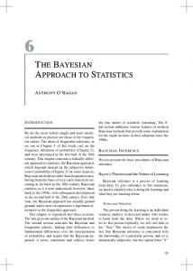
Results: differentially expressed genes

40

The method finds 24 differentially expressed genes out of 2887 analysed genes. | | |

|

| |

30

|

| |

|

| | |

20

| |

| |

|

|

|

10

|

|

|

|

|

|

| | |

|

| |

|

| |

| 0

genes

| |

| |

|

|

| | | | | |

−0.5

0.0

0.5

1.0

1.5

2.0

2.5

3.0

CI – p. 11

Tseng’s model We compared our results with whose obtained with Tseng et al. model on the same data. First we normalised the data externally (Yang et al., 2002). Then the normalised logratio intensities were modelled as ygs ∼ N (θg , σg2 ) θg ∼ N (µθg , σθ2g ) and the hyperparameters µθg , σθ2g had a non informative distribution. The distribution of σg2 is the following σg2

=

wg χ2g k

where k is the number of degree of freedom for the chi squared. wg is a weighted value from the gene-specific and overall variance calculated on the calibration arrays data. – p. 12

Results: comparisons The Tseng et al model found 47 differentially expressed genes out of 2887 analysed genes. Our model

Tseng’s model

2

25 22

24

47

Tseng’s model found 27 down regulated genes out of 47, while our method found only 2 differentially negative expressed genes.

– p. 13

50

Results: comparisons ||

|| || || |

20

genes

30

40

| | || || | | | | || || | | || | | | | | | | || | || | | || || || | | | | |

10

|| |

0

|

−1

||

|

|| ||

|| | | ||| | ||| 0

|

||

|

| || || | | ||| | | | ||| || | | |

| | || || | | || |

|| | ||| | | | | | | || || | |

|

|

|

| | |

|

|

| | || | 1

2

3

4

CI – p. 14

..with the same normalisation

40

To investigate the differences in the results we introduced in Tseng’s et al. model the normalisation inside the model. We found 40 differentially expressed genes:

20 −0.5

0.0

10 |

| | | | | || | | | | || |

0

genes

30

||

| | || | | | || | | || || | || | || || | | | | |

||

||

| | | | || | | | | || | | | | | || | | | | | | | || | 0.5

||

||

| | || | || || | || | | | || || | | | | | | | | | || ||

1.0

1.5

|| | |

2.0

||

2.5

3.0

CI – p. 15

Biological results

– p. 16

Biological results

– p. 17

Discussion Use a fully Bayesian approach: flexible Normalisation as a part of the model: allow to control the noise in the signals Using self self experiment: allows to model the variability on the expression intensity level, as well as on the normalised logratio level as informative. Statistical information on the variability hyperparameters: allows to include and analyse genes that are present in comparative experiments, even if they are missing in self self experiments. Useful to be followed when considering a sequence of experiments: it permits to update prior information and to take under control sources of variations that can be introduced between different experiments. – p. 18

Further works Our model and Tseng’s et al. one differ for 14 upregulated genes.

– p. 19

Further works Our model and Tseng’s et al. one differ for 14 upregulated genes. Deeper analysis to investigate these different results

– p. 19

Further works Our model and Tseng’s et al. one differ for 14 upregulated genes. Deeper analysis to investigate these different results Linear normalisation: doesn’t capture non linear effects.

– p. 19

Further works Our model and Tseng’s et al. one differ for 14 upregulated genes. Deeper analysis to investigate these different results Linear normalisation: doesn’t capture non linear effects. Introduce a non linear normalisation as part of the model

– p. 19

Further works Our model and Tseng’s et al. one differ for 14 upregulated genes. Deeper analysis to investigate these different results Linear normalisation: doesn’t capture non linear effects. Introduce a non linear normalisation as part of the model Too many parameters on τg effects

– p. 19

Further works Our model and Tseng’s et al. one differ for 14 upregulated genes. Deeper analysis to investigate these different results Linear normalisation: doesn’t capture non linear effects. Introduce a non linear normalisation as part of the model Too many parameters on τg effects Use of mixture models, even with an unspecified number of components.

– p. 19

References Lewin A., Richardson S., Marshall C., Glazier A. and Aitman T. (2003) Bayesian modelling of differential gene expression, submitted. Pepe G., Giusti B., Attanasio M., Gori A., Comeglio P., Martini F., Gensini G., Abbate R. and Neri Sernieri G. (1997) Tissue factor and plasminogen activator inhibitor type 2 expression in human stimulated monocytes is inhibited by heparin, Seminars in Thrombosis and Hemostasis, 23, 2, 135–145. Simon R., Korn E. and McShane L. (2003) Design and Analysis of DNA Microarray Investigations, Springer-Verlag. Spiegelhalter D., Thomas A., Best N. and Lunn D. (2003) WinBUGS, version 1.4., MRC Biostatistics Unit, Cambridge, UK. Tseng G., Oh M., Rohlin L., Liao J. and Wong W. (2001) Issues in cDNA microarray analysis: quality filtering, channel normalization, models of variations and assessment of gene effects, Nucleic Acids Research, 29, 2549–2557. Yang Y., Dudoit S., Luu P., Lin D., Peng V., Ngai J. and Speed T. (2002) Normalization for cDNA microarray data: a robust composite method addressing single and multiple slide systematic variation., Nucleic Acids Research, 30, 4.

19-1