A Bayesian Computational Cognitive Model - CEUR-WS.org

A Bayesian Computational Cognitive Model ∗ Zhiwei Shi Hong Hu Zhongzhi Shi Key Laboratory of Intelligent Information Processing Institute of Computing Technology, CAS, China Kexueyuan Nanlu #6, Beijing, China 100080 {shizw, huhong, shizz}@ics.ict.ac.cn Abstract Computational cognitive modeling has recently emerged as one of the hottest issues in the AI area. Both symbolic approaches and connectionist approaches present their merits and demerits. Although Bayesian method is suggested to incorporate advantages of the two kinds of approaches above, there is no feasible Bayesian computational model concerning the entire cognitive process by now. In this paper, we propose a variation of traditional Bayesian network, namely Globally Connected and Locally Autonomic Bayesian Network (GCLABN), to formally describe a plausible cognitive model. The model adopts a unique knowledge representation strategy, which enables it to encode both symbolic concepts and their relationships within a graphical structure, and to generate cognition via a dynamic oscillating process rather than a straightforward reasoning process like traditional approaches. Then a simple simulation is employed to illustrate the properties and dynamic behaviors of the model. All these traits of the model are coincident with the recently discovered properties of the human cognitive process.

1

Introduction

One of the most fundamental issues in cognitive science is knowledge representation. Different strategies lead to different cognitive models. Symbolic approaches, which have relative long tradition, adopt the symbolic concept representation, and employ the rule-based reasoning to construct intelligent systems. This approach is often referred to as the classical view [Russel and Norvig, 1995]. In contrast, connectionist approaches, which emerge relative later, utilize neural networks to perform parallel process on the distributed knowledge representation. Besides the conceptual and implemental differences, all these models exhibit excellent

problem solving capability and provide meaningful insights into mechanisms of human intelligence. Besides the two categories of models, recently, there emerges a novel approach, hybrid neural-symbolic system, which concerns the use of problem-specific symbolic knowledge within the neurocomputing paradigm [d'Avila Garcez et al., 2002]. This new approach shows that both modal logics and temporal logics can be effectively represented in artificial neural networks [d'Avila Garcez and Lamb, 2004]. Different from the hybrid approach above, we adopt Bayesian network [Pearl, 1988] to integrate the merits of rule-based systems and neural networks, due to its virtues as follows. On the one hand, by encoding concepts as nodes and causal relationship between concepts as directed links, BN can manipulate symbolic concepts and perform inference, reasoning and diagnose; on the other hand, the graphical structure enables it to implement neural mechanisms in the brain, which is previously the privilege of neural networks. Furthermore, the probabilistic architecture endows BN the capability of performing reasoning based on incomplete information, which is often the case in cognitive tasks. More importantly, as Judea Pearl [Pearl, 1997] mentioned, “a Bayesian network constitutes a model of the environment rather than, as in many other knowledge representation schemes (e.g., rule-based systems and neural networks), a model of the reasoning process, and it simulates, in fact, the mechanisms that operate in the environment, and thus facilitates diverse models of reasoning, including prediction, abduction and control”. This is extremely significant, because, according to the isomorphism1 of the Gestalt Theory, the brain field of human beings should have the similar structure with that of the external circumstance, which is reflected by the internal cognitive model. Therefore, modeling the environment is a key point towards constructing considerable cognitive models.

1

∗

This work is supported by the National Science Foundation of China (No. 60435010, 90604017, 60675010), National Basic Research Priorities Programme No. 2003CB317004 and the Nature Science Foundation of Beijing No. 4052025.

In mathematics an isomorphism between two systems requires a one-to-one correspondence between their elements (that is, each element of one system corresponds to one and only one element of the other system, and conversely), which also preserves structures. In Gestalt psychology, the one-to-one correspondence between elements is not required; similarity of structures is required [Luchins and Luchins, 1999].

Although many Bayesian cognitive models (see e. g. [George and Hawkins, 2005; Lee and Mumford, 2003]) are carried out, they all focus on some specific aspects of cognition. No overall cognitive architecture based on BN has been proposed by now, mainly due to the inherent limitations of the BN. The primary limitation is about incomplete data. An overall cognitive model based on BN will involve numerous nodes/concepts. Yet, each piece of an observation contains only a tiny part of the external world, as well as its reflection in the cognitive model. It is absolutely impossible to have a completed sample of all the concepts of an overall model within just one observation. This means that the task of learning Bayesian network will inevitably depend on techniques of learning with incomplete data. Although, in the last decade, with the rapid progress in researches on BN, many algorithms (see e.g. [Friedman, 1997; Ramoni and Sebastiani, 2001]) have been developed to deal with the incomplete data in the learning of BN, the proportion of missing data in their researches is less than 50%. Therefore, in cases that only several concepts are observed with millions of concepts missing, their methods will definitely become powerless. The second problem is about directed links. In a BN, edges between nodes are one-way directed. Yet, interrelationships between concepts, which exist in the real world and can be reflected in the cognitive model, are sometimes bidirectional. In these cases, the original BN is incapable due to its inherent limitation. The last point comes from the feasibility. The problem of learning an exact Bayesian network from data under certain broad conditions has been proven worst-case NP-hard [Chickering et al., 2003]. Although researchers have proposed heuristic polynomial learning algorithms [Brown et al., 2005] to alleviate the work, it is still computationally intractable for dealing with the problem with millions of nodes in the domain. Based on the analyses above, we get that it is not wise to exploit a huge global BN to construct a cognitive model. Consequently, we propose a variation of BN, Globally Connected and Locally Autonomic Bayesian Network (GCLABN), which is composed of numerous interconnected and overlapped tiny Bayesian networks, to model the overall cognition. The rest of this paper is organized as follows: in Section 2, we will introduce the novel cognitive model, GCLABN, in detail and discuss some important issues of the model; then we employ a simple simulation to illustrate the properties of the proposed model in Section 3; finally, we conclude our paper in section 4 with a short review of our work and possible directions in the future.

2

The GCLABN Model

2.1 Model Description Before we come to the GCLABN model, we firstly introduce some necessary definitions. Definition 2.1 In a directed acyclic graph G = (V, E), a node C ∈ V is called a center node if and only if for any

node X ∈ V\{C}, the edge ∈ E is satisfied2. For example, in Fig. 1, node n2 in graph G1 and node n3 in graph G2 are all center nodes in their graphs respectively. Definition 2.2 A directed acyclic graph is a centered graph if and only if it has only one center node, and there is no edges ending at non-center nodes. For example, graph G1 in Fig. 1 is a centered graph, and graph G2 is not due to the extra edges between non-center nodes. The center node of a centered graph is specified shortly to C(G). So, in Fig. 1, we have C(G1) = n2. n1

n1

n2

n3

n2

n3

n4

n4

n5

G1

G2

Fig.1. The Sample Graphs

Definition 2.3 A centered Bayesian network (CBN) is a pair (G, P), where G = (V, E) is a centered graph, and P is a set of conditional probabilistic distribution (CPD) of the center node of G given its parents. For convenience, we also call the center of G, C(G), the center of CBN, shortly for C(CBN). Definition 2.4 For any two given centered Bayesian network B1 = (G1, P1) and B2 = (G2, P2), if C(B1) ≠ C(B2), the union B = B1∪B2 of CBN B1 and CBN B2 is a pair (G, P), where G is the union of G1 and G2, and P is the union of P1 and P2. n1

n5

……

……

n2

n3

B1

n4

B2

n6

B = B1∪B2

Fig.2. The union of two CBNs

Fig. 2 illustrates a sample union of two CBNs. From this figure, we can see that, in the left oval is one CBN B1 = (G1, P1), whose edge is solid arrowed lines, and in the right oval is the other CBN B2 = (G2, P2), whose edge is dot arrowed line. For G1 = (V1, E1), we have V1 = {n1, n2, n3, n4} and E1 = {n1 →n2, n3→n2, n4→n2}; for G2 = (V2, E2), we have V2 = {n2, n4, 2

Here X is the start point of the edge.

n5, n6} and E2 = {n2→n4, n5→n4, n6→n4}. The union of B1 and B2 , B, is also a labeled graph model, whose graph structure is G = (V, E), where V = { n1, n2, n3, n4, n5, n6} and E = {n1→n2, n3→n2, n4→n2, n2→n4, n5→n4, n6→n4}. The CPD set P of B is the union of P1 and P2, which are the CPD sets of B1 and B2 respectively. Definition 2.5 A globally connected and locally autonomic Bayesian network (GCLABN) is a union, GCLABN = B1 ∪B2 ∪…∪Bn, where Bi (i = 1, …, n) are centered Bayesian networks, and they are subject to the following constraints:

C ( Bi ) ≠ C ( B j ) 1 ≤ i < j ≤ n

(1)

C ( Bi ) ∈ (UV j ) i = 1, K, n

(2)

and j ≠i

where Vj is the node set of Bj. The first constraint makes every CBN unique. The second constraint makes all the CBNs connected in terms of center nodes. From the definition, we can see that a GCLABN is composed of many interconnected and overlapped CBNs. To some extent, a GCLABN is just like a Cellular Automata (CA). The difference is that all the cells in a CA are homogeneous, while CBNs in a GCLABN are heterogeneous. Besides, the topology of a CA is regular network, while the topology of a GCLABN is not. According to Definition 2.5, we get that GCLABN can represent bidirectional relationship (see Fig. 2 e.g., there are links from node n2 to n4 and vice versa.). Hence, GCLABN successfully solve the problem in BN that one-way directed link cannot represent bidirectional relationship.

2.2 GCLABN as Cognitive Model When a GCLABN is employed as a cognitive model, all its nodes, each of which can be viewed as a neuron, or a functional neural column [Gilbert and Wiesel 1989], or the like, represent the concepts that can be learnt from the external world. Each node takes two states, i.e. ‘1’ for active and ‘0’ for inactive. At any time instant, the probability of state ‘1’ for any given node indicates its current active strength. The directed links, which can be viewed as the connections between neurons, encode direct causal relationships between concepts. Before we make further discussions on GCLABN, we divide all the nodes of a GCLABN into two categories, where center nodes of CBNs are called internal nodes and the other nodes are called external nodes. The external nodes represent concepts that can be identified by the model directly, or without any inference. They serve as the sensory interface of the model. While internal nodes encode high-level concepts, which can be activated only after inference. They deal with information manipulating or some motor tasks.

2.3 CPDs of GCLABN One of the most important issues of GCLABN is about the Conditional Probabilistic Distributions (CPDs) of internal nodes, for the CPDs of a given node defines the updating rule of its active strength and CPDs of all the internal nodes

formulate how the state of a GCLABN varies given the outside inputs. Since each node in GCLABN takes two states, the CPDs of an internal node with N parent nodes will contain 2N entries, e.g. 100 parents correspond to about 1030 entries. It is unimaginable for a neuron to implement such mechanism. Fortunately, the human cerebral structure provides us a hint. As we all know, the entire cerebrum of a human is divided into many functional regions. Each region specializes in some specific function, and neurons in the same functional region carry out similar function. Accordingly, all the nodes of a GCLABN can be clustered into many distinct regions based on the functional similarity between nodes. Thus, to simplify the CPDs of a node in the GCLABN, we import the following two assumptions. The first assumption is that all the nodes in a same region are mutually exclusive, and they compete to be activated. This assumption is referred to as the exclusive competition. Under this assumption, for each region R = {x1, …, xnR}, we have: nR

P( R) = ∑ P( xk )

( 3)

k =1

Note: for P(R) is not larger than 1, all the P(xk) in the same region are normalized. This normalization process can be interpreted as lateral inhibitory effects between neurons, or neural columns. The second assumption is that, for any given node, its parent nodes from different regions produce independent influences. We refer the second assumption as the regional casual independence, which can be formalized as formula 4.

P ( x | R1 , L, Rn ) = P ( x | R1 ) L P ( x | Rn )

( 4)

where x is the target internal node, and Ri (i = 1, 2, …, n) is the region that contains its parent nodes. According to the first assumption, P(x|Ri) can be written as: nk

P ( x | Ri ) = ∑ P ( x | xik ) P ( xik | Ri ) i = 1,L , n

( 5)

k =1 nk

= ∑ P( x | xik ) P( xik ) P ( Ri )

( 6)

k =1

where Ri = {xi1, …, xini} (i = 1, 2, …, n) is the region that contains parent nodes of the target node x. Thus, based on formula 3, 4 and 6, we can easily calculate the probability, or active strength, of any internal node given the status of its parent nodes: n

nk

P ( x | R1 ,L , Rn ) = ∏∑ P ( x | xik ) P( xik ) P( Ri )

( 7)

i =1 k =1

Based on formula 7, we successfully reduce the size of CPDs from O(2N) to O(N).

2.4 Learning a GCLABN Since a GCLABN is composed of many interconnected but autonomic CBNs, the learning task of the model can be divided into many independent tiny learning tasks. Each task just focuses on one local CBN. Compared with ordinary BN, learning a CBN is much simpler, because the network

structure of any CBN is almost fixed (all edges pointing to the center node from its parent nodes), and the CPDs of the center node can be leant based on Hebb rules. As a result, the learning process is not NP hard as the original BN. Besides, local learning strategy avoids the missing data problem as well.

2.5 Generating Cognition The key issue of a cognitive model is to generate cognition according to external inputs. Different from traditional symbolic approaches and neural networks, whose reasoning process is straightforward, the inference task in GCLABN is completed via a dynamic oscillating process. After a GCLABN receives external stimuli via its external nodes, at each time instant, all the internal nodes modified their active strengths according to the states of their parent nodes and their own CPDs (see formula 7). As time goes by, the states of all the internal nodes vary continually. After a period of oscillation, the process will converge to a stationary point, which is called as an “attractor” in the dynamical perspective. At this time, the champion nodes of all the regions connected to the active external nodes in GCLABN together form the current cognition. As we stated above, in GCLABN, external nodes serve as sensors to receive outside inputs. Although there are no nodes in GCLABN explicitly in charge of outputting, given external inputs and after a period of inference, champion nodes in all the regions of GCLABN together represent the cognitive result. During the dynamic cognition generating process, GCLABN demonstrates the capability of both manipulating symbolic concepts and implementing neural mechanisms. On one hand, from the symbolic perspective, after filtering out irrelevant concepts during oscillation, winners represent all the concepts involved in the reasoning process, including preconditions, intermediary results, and final conclusions. Since directed links in GCLABN encode direct causal relationships, the “outputs” of GCLABN virtually provide the symbolic reasoning process as well. On the other hand, from the neural perspective, the cognition process is a dynamic process, and the champion neuron assembly, other than a single neuron alone, represents the cognitive results. This is quite coincident with many neurobiological experimental results [Beer 2000; Engel et al., 2001]. One slight, but very important, difference between GCLABN and common dynamical systems is that in GCLABN there are some external nodes, whose status is neither stochastic nor determined by their parents. They are totally affected by the environment. Thus, once statuses of external nodes are changed due to the transformation of external circumstance, GCLABN will escape from the previous "attractor" and start a new cognitive process.

3 Simulation In this section, we employ a simple simulation to illustrate the properties of a GCLABN. When people perform cognition in the real world, information gained from sensors is usually incomplete compared

with the knowledge stored in the brain. For example, the knowledge about a concept, e.g. an apple, in the brain may involve visual information, aural information, tactual information and so forth; yet in a cognition task, only a small portion of information is available and cognition will be generated based on the incomplete information. Thus, in our simulation, we adopt a word/sentence recognition test based on incomplete inputs to demonstrate the capability and behavior of GCLABN in cognition. In the simulation, we firstly mimic Elman’s work [Elman, 1990] to generate 10000 two-word or three-word sentences with a sentence generator program, which utilizes 29 different lexical items and 16 sentence templates 3 . Then a sample GCLABN is learnt according to these 10000 sentences. After that, different from Elman’s simulation, where the task of predicting the following word is performed, we give some incomplete words and sentences to the GCLABN for recognition. Finally, we examine the "outputs” of the model and its dynamical behavior during the process of cognition making.

3.1 Knowledge Representation In this sample GCLABN, different internal nodes represent distinct words; external nodes represent the letters that compose the words; directed links denote either sequential relationships between words in sentences or composition relationships between words and letters; the probability of each node implies its active strength (0 for completely inactive and 1 for extremely active). Yet, to represent the spatial information, which indicates the position of a word in a sentence, we import three extra internal nodes to denote different positions in a sentence. These position nodes will not be activated simultaneously, and all the word nodes, which are active with a position node concurrently, will form a virtual region and compete to become prominent. For simplicity, in this model there is no node representing a whole sentence.

3.2 Learning Process In this process, all the sentences are processed one pass sequentially. After each sentence is read, related words and letters are recorded as new nodes if they are not in the model yet; then composition relationships between words and corresponding letters and sequential interrelationships between words are interpreted as directed links if not existing; at last related statistical parameters in the model is either created or updated. For example, after the first sentence "girl eat cookie" is read, three new internal nodes, corresponding to "girl", "eat" and "cookie" respectively, are constructed together with necessary external nodes corresponding to letters. Links between word nodes "girl → eat" and "eat → cookie" and links between word nodes and letter ones, are added to the model. For sake of the model simplicity, we do not encode the link "girl → cookie", although interrelationships between subjects and objects are also informative. 3

For detailed information of the word categories and the sentence templates, please see [Elman, 1990] for reference.

3.3 Word/Sentence Recognition

3.4 Dynamical Property

After the GCLABN is learnt, we perform a word/sentence recognition test. First of all, we randomly erase some words in the sentences we generated and leave only one letter for each erased word as a cue4. For example, “-r -t cookie” is the incomplete version of “girl eat cookie”, where ‘-’ indicates a fragmentary word. Then, the model is asked to recognize the words and sentences based on the incomplete information. After that, we evaluate the recognition performance in terms of both words and sentences. For word level performance, we examine the total correctly recognized words in the task. In the sentence level verification, if a recognized sentence matches one of the templates, which are used to generate these sentences, the recognition is successful. Otherwise, the recognition is a failure. To make a contrast, we also exploit a purely bottom-up strategy, which is adopted by many traditional approaches. The bottom-up recognition model identifies the incomplete words/sentences merely according to the letter cues. Table 1 and table 2 show the evaluation result.

As we mentioned in the previous section, the cognition generating

Table2: Sentence level performance Recognition strategy GCLABN Bottom-up Correct number 6129 3644 Correct rate 93% 55% Total incomplete sentences 6601 6601

active strength

0.7 0.6

mouse

0.5

man

0.4

smash

0.3

move

0.2

monster

0.1

woman

0 1

2

3

4

4

In this process, each word is selected at the probability of 1/3 for erasing; for each erased word, all its letters have equal possibility to be remained as the cue. 5 Interestingly, the GCLABN has learnt the word categories, as well as the sentence template, during the learning process. Yet, due to the space limitation, we do not provide further discussion on this issue.

6

7

8

9

10 11 12

smell

(a) The dynamical process at position 1 mouse

1.2

smash

1

glass

0.8

sandwich

0.6

see

0.4

monster

0.2

smell exist

0 1

2

3

4

5

6

7

8

9

10 11 12

Time instant

From the two tables we can see that at the both levels the

chase sleep

(b) The dynamical process at position 2 cookie

1.2

mouse

1

active strength

GCLABN outperforms the purely bottom-up strategy greatly, especially at the sentence level. Clearly, interactions between internodes during the cognitive process facilitate the cognition in the cases that the external information is insufficient. As a matter of fact, if in the learning process the model encodes more information, e.g. subject-object relationships, the performance of cognition will be even better. Besides, if we teach the GCLABN word categories and sentence template knowledge5, and the model performs another pass of learning, the performance will also be improved. Furthermore, we also notice that the GCLABN achieves better accuracy in the sentence level verification. In contrast, the bottom-up method encounters more difficulties when dealing with the sentences as a whole. Therefore, although we do not teach the GCLABN any syntactic knowledge, the interrelationship between concepts has already encoded some syntactic information, according to the experimental result.

5

Time instant

active strength

Table1: Word level performance Recognition strategy GCLABN Bottom-up Correct number 8023 6875 Correct rate 89% 76% Total incomplete words 9015 9015

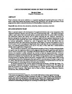
process in GCLABN is a dynamic oscillating process. Hence, we illustrate one sample oscillating process during the word/sentence recognition task as follows. In Fig. 3, the dynamical process of recognizing incomplete sentence “-m -s -o”, which comes from the original sentence “man smell book”, is presented.

book 0.8

lion boy

0.6

dog 0.4

move dragon

0.2

rock

0 1

2

3

4

5

6

7

8

Time instant

9

10

11

12

monster woman

(c) The dynamical process at position 3 Fig. 3 The dynamical process of cognizing the sentence “-m -s –o”, where the final cognitive result is the sentence “man smell book”

From Fig. 3, we can see that although the initial active strengths of the candidate nodes, which are purely determined by the external inputs, are quite similar, as time goes by, with the interaction between the internal nodes, some candidates become prominent very soon (see Fig. 3a and 3b). This means: although input information is very limited in some cognitive tasks, with the pre-learnt knowledge and

other related information gained in the same scene, GCLABN can eventually figure out what it is. While, we also notice that at some position, there are several competitive candidates. See Fig.3a for example, the word “man” and “woman” are quit competitive, and it is hard to decide which one is the winner in very short time oscillation. This gives computational explanation of why sometimes people fail in a dilemma due to less information plus indiscriminative knowledge structure.

4

Conclusion

In this paper, we propose a Bayesian computational cognitive model, Globally Connected and Locally Autonomic Bayesian Network (GCLABN), accompanied by a simple simulation to illustrate its properties. The novel model possesses many attractive traits. Firstly, it employs a unique knowledge representation strategy within a graphical structure, where symbolic concepts are encoded as nodes, relationships between concepts are represented as directed links, and strengths of relationships are stored as CPDs. Secondly, by generating cognition via dynamic oscillation, it integrates the merits of both the symbolic approaches and the connectionist approaches. On the one hand, the GCLABN provide a white-box architecture by manipulating the symbolic concepts with probabilistic reasoning (Formula 7); on the other hand, the graphical structure enables the GCLABN to implement some neural mechanisms in the brain, e.g. neural assembly theory and dynamic oscillation (see Fig. 3). Last, but not least, the GCLABN, like traditional BN, models the environment rather than performs specific problem solving. By this means, it possesses more general problem solving capability. Before we end up this paper, we have to point out that the model is far from fully developed. There are still some important issues deserving further research. For example, how to divide the entire GCLABN into different functional regions? Is it necessary to make regions explicitly? How to perform communication between different GCLABN models? At what abstract level should sensory nodes be placed? For instance, in our simulation, should a sensory node represent a word, or a letter, or some low-level visual stimulus? How can links fade out, so that the model can filter out the input noises like the human beings? So, actually we propose more questions than offer a complete solution. To sum up, our work makes a meaningful attempt to model the cognition in the brain, and we hope it can open up a new avenue for the study of the computational model of the cerebrum or even constructing an artificial brain.

References [Beer, 2000] Randall D. Beer. Dynamical approaches to cognitive science. Trends in Cognitive Sciences, 4(3): 91-99, March 2000. [Brown et al., 2005] L.E. Brown, I. Tsamardinos and C.F. Aliferis. A Comparison of Novel and State-of-the-Art Polynomial Bayesian Network Learning Algorithms, In Proceedings of AAAI 2005, pages 739-745, 2005.

[Chickering et al., 2003] D. Chickering, C. Meek and D. Heckerman. Large-sample learning of bayesian networks is np-hard. In Proceedings of the 19th Annual Conference on Uncertainty in Artificial Intelligence (UAI-03), pages 124-133, 2003. [d'Avila Garcez and Lamb, 2004] Artur S. d'Avila Garcez and Luis C. Lamb. Reasoning about Time and Knowledge in Neural-Symbolic Learning Systems. In Advances in Neural Information Processing Systems 16, Proceedings of the NIPS 2003 Conference, MIT Press, 2004. [d'Avila Garcez et al., 2002] Artur S. d'Avila Garcez, Krysia Broda and Dov M. Gabbay. Neural-Symbolic Learning Systems: Foundations and Applications, Perspectives in Neural Computing, Springer-Verlag, 2002. [Elman, 1990] J.L. Elman. Finding structure in time. Cognit. Sci. 14: 179-211, 1990. [Engel et al., 2001] A.K. Engel, P. Fries, and W. Singer. Dynamic predictions: oscillations and synchrony in top-down processing. Nature Rev. Neurosci. 2: 704-716, 2001. [Friedman, 1997] N. Friedman. Learning Belief Networks in the Presence of Missing Values and Hidden Variables. In Proceedings of the Fourteenth International Conference on Machine Learning, pages 125-133, San Francisco, CA, USA, 1997. [George and Hawkins, 2005] D. George and J. Hawkins. A hierarchical Bayesian model of invariant pattern recognition in the visual cortex. In Proceedings of the International Joint Conference on Neural Networks, 2005. [Gilbert and Wiesel, 1989] C. D. Gilbert and T. N. Wiesel. Columnar specificity of intrinsic horizontal and corticocortical connections in cat visual cortex. Journal of Neuroscience, 9:2432-2442, 1989. [Lee and Mumford, 2003] T. S. Lee and D. Mumford. Hierarchical Bayesian inference in the visual cortex. Journal of the Optical Society of America 2(7): 1434-1448, 2003. [Luchins and Luchins, 1999] A.S. Luchins and E.H. Luchins Isomorphism in Gestalt Theory: Comparison of Wertheimer's and K?hler's Concepts. GESTALT THEORY, 21(3): 208-234, Nov. 1999. [Pearl, 1988] J. Pearl. Probabilistic Reasoning in Intelligent Systems: Networks of Plausible Inference. Morgan Kaufmann, San Mateo, California, 1988. [Pearl, 1997] J. Pearl. Bayesian Networks. Technical Report R-246 (Rev. II), October 1997. To appear in MIT Encyclopedia of the Cognitive Sciences. [Ramoni and Sebastiani, 2001] M. Ramoni and, P. Sebastiani. Robust learning with missing data. Machine Learning, 45(2): 147-170, 2001. [Russel and Norvig, 1995] S. Russell and P. Norvig. Artificial Intelligence: A Modern Approach. Prentice-Hall, Upper Saddle River, NJ, 1995.