Hydrol. Earth Syst. Sci., 10, 413–426, 2006 www.hydrol-earth-syst-sci.net/10/413/2006/ © Author(s) 2006. This work is licensed under a Creative Commons License.
Hydrology and Earth System Sciences
A Bayesian decision approach to rainfall thresholds based flood warning M. L. V. Martina, E. Todini, and A. Libralon Dept. of Earth and Geo-Environmental Sciences, Univ. of Bologna, Piazza di Porta San Donato, 1, Bologna, 40126, Italy Received: 13 October 2005 – Published in Hydrol. Earth Syst. Sci. Discuss.: 13 December 2005 Revised: 31 March 2006 – Accepted: 1 April 2006 – Published: 7 June 2006
Abstract. Operational real time flood forecasting systems generally require a hydrological model to run in real time as well as a series of hydro-informatics tools to transform the flood forecast into relatively simple and clear messages to the decision makers involved in flood defense. The scope of this paper is to set forth the possibility of providing flood warnings at given river sections based on the direct comparison of the quantitative precipitation forecast with critical rainfall threshold values, without the need of an on-line real time forecasting system. This approach leads to an extremely simplified alert system to be used by non technical stakeholders and could also be used to supplement the traditional flood forecasting systems in case of system failures. The critical rainfall threshold values, incorporating the soil moisture initial conditions, result from statistical analyses using long hydrological time series combined with a Bayesian utility function minimization. In the paper, results of an application of the proposed methodology to the Sieve river, a tributary of the Arno river in Italy, are given to exemplify its practical applicability.
1 Introduction 1.1
The flood warning problem
The aim of any flood warning system is to provide useful information to improving decisions such as for instance issuing alerts or activating the required protection measures. Traditional flood warning systems are based on on-line hydrological and/or hydraulic models capable of providing forecasts of discharges and/or water stages at critical river sections. Recently, flood warning systems have also been coupled with quantitative precipitation forecasts (QPF) gener-
ated by numerical weather models (NWM), in order to extend the forecasting horizon from a few hours to a few days (EFFS, 2001–2004). Consequently, flood forecasting systems tend to require hydrological/hydraulic models to run in real time during flood emergencies, with increasing possibility of system failures due to several unexpected causes such as model instabilities, wrong updating procedures, error propagation, etc. In several countries operational flood management rests with professional who have the appropriate technical background to interpret all of the information provided by the real-time flood forecasting chain. However, in many other cases, the responsibility of issuing warnings or to take emergency decisions rests with non hydro-meteorology knowledgeable stakeholders, this is the case for instance of flood emergency managers or mayors. The aim of this paper is to explore the possibility of issuing flood warnings by directly comparing the forecast QPF to a critical rainfall threshold value incorporating all the important aspects of the problem (initial soil moisture conditions as well as expected costs), without the need to run the full chain of meteorological and hydrological/hydraulic real time forecasting models. Although it should not be considered as an alternative to the comprehensive hydro-meteorological forecasting chain, due to the simplicity of the final product (a couple of graphs), this approach can be an immediate tool for non purely technical decision makers in the case of early warnings and flash floods. Apart from their extensive use in the United States (Georgakakos, 2006) and in Central America, in Europe, the Integrated Project FLOODSite (http://www.floodsite.net) among others aims at assessing the advantage for using the rainfall threshold approach as an alternative to the traditional ones in the case of flash floods.
Correspondence to: M. L. V. Martina (
[email protected]) Published by Copernicus GmbH on behalf of the European Geosciences Union.
414
M. L. V. Martina et al.: Bayesian rainfall thresholds
Fig. 1. Example of a rainfall threshold and its use.
1.2
The rainfall threshold approach
The use of rainfall thresholds is common in the context of landslides and debris flow hazard forecasting (Neary et al., 1986; Annunziati et al., 1996; Crosta and Frattini, 2000). Rainfall intensity increases surface landslide hazard (Crosta and Frattini, 2003) while soil moisture content affects slope stability (Iverson, 2000; Hennrich, 2000; Crosta et Frattini, 2001). In the context of flood forecasting/warning, rainfall thresholds have been generally used by meteorological organizations or by the Civil Protection Agencies to issue alerts. For instance, in Italy an alert is issued by the Civil Protection Agency if a storm event of more than 50 mm is forecast for the next 24 h over an area ranging from 2 to 50 km2 . Unfortunately, this type of rainfall threshold, which does not account for the actual soil saturation conditions at the onset of a storm event, tends to heavily increase the number of false alarms. In order to analyze flood warning rainfall thresholds in more detail, following the definition of thresholds used for landslides hazard forecast, let us define them as “the cumulated volume of rainfall during a storm event which can generate a critical water stage (or discharge) at a specific river section”. Figure 1 shows an example of rainfall thresholds i.e. accumulated volume of rain versus time of rainfall accumulation. In order to establish the landslides warning thresholds, De Vita and Reichenbach (1998) use a number of statistics (such as the mean), to be derived from long historical records, of the amount of precipitation that happened immediately before the event. Mancini et al. (2002), as an alternative to the use of historical records in the case of floods, proposed an approach based on synthetic hyetographs with different shapes and durations for the estimation of flood warning rainfall thresholds. The threshold values are estimated by trial and error with an event based rainfall-runoff model, as the value of rainfall producing a critical discharge or critical water stage. Although the Mancini et al. (2002) approach overcomes the limitations of the statistical analysis based exclusively on Hydrol. Earth Syst. Sci., 10, 413–426, 2006
historical records, rarely sufficiently long to produce statistically meaningful results, it presents some drawbacks due to the use of an event based hydrological model. In particular, it requires assumptions both on the temporal evolution of the designed storms and on the antecedent moisture conditions of the catchment, which one would like to avoid. A rainfall threshold approach has also been developed and used within the U.S. National Weather Service (NWS) flash flood watch/warning programme (Carpenter et al., 1999). Flash flood warnings and watches are issued by local NWS Weather Forecast Offices (WFOs), based on the comparison of flash flood guidance (FFG) values with rainfall amounts. FFG refers generally to the volume of rain of a given duration necessary to cause minor flooding on small streams. Guidance values are determined by regional River Forecast Centers (RFCs) and provided to local WFOs for flood forecasting and the issuance of flash flood watches and warnings. The basis of FFG is the computation of threshold runoff values, or the amount of effective rainfall of a given duration that is necessary to cause minor flooding. Effective rainfall is the residual rainfall after losses due to infiltration, detention, and evaporation have been subtracted from the actual rainfall: it is the portion of rainfall that becomes surface runoff at the catchment scale. The determination of FFG value in an operational context requires the development of (i) estimates of threshold runoff volume for various rainfall durations, and (ii) a relationship between rainfall and runoff as a function of the soil moisture conditions to be estimated for instance via a soil moisture accounting model (Sweeney et a., 1992). As applied in the USA, approaches for determining threshold runoff estimates varied from one RFC to another, and in many cases, were not based on generally applicable, objective methods. Carpenter et al. (1999) developed a procedure to provide improved estimates of threshold runoff based on objective hydrologic principles. For any specific duration, the runoff thresholds are computed as the flow causing flooding divided by the catchment area times the Unit Hydrograph peak value. The procedure includes four methods of computing threshold runoff according to the definition of flooding flow (two-year return period flow or bankfull discharge) and the methodology to estimate of the Unit Hydrograph peak (Synder’s synthetic Unit Hydrograph or Geomorphologic Unit Hydrograph). A Geographic Information System is used to process digital terrain data and to compute catchment-scale characteristics (such as drainage area, stream length and average channel slope), while regional relationships are used to estimate channel cross-sectional and flow parameters from the catchment-scale characteristics in the different locations within the region of application. However the quality of the regional relationships, along with the assumptions of the theory, limits the applicability of the approach. For example, the assumption that the catchment responds linearly to rainfall excess, which is needed to apply the unit hydrograph theory, imposes lower limits on the size of the catchment, as small catchments are more non-linear www.hydrol-earth-syst-sci.net/10/413/2006/
M. L. V. Martina et al.: Bayesian rainfall thresholds than larger ones (Wang et al., 1981). But at the same time, the assumption of uniform rainfall excess over the whole catchment implicitly introduces upper bounds on the size of the catchments where a Unit Hydrograph approach could be considered reasonable. Furthermore, the assumption of uniform rainfall excess over the catchment also implicitly limits the size of the catchment for which a unit hydrograph approach is reasonable. With reference to the second aspect of the FFG, namely the estimation of the relationship between rainfall and runoff as a function of the soil moisture conditions, in a recent paper Georgakakos (2005) derives a relationship between actual rainfall and runoff, which is taken equal to the effective rainfall, both for the operational Sacramento soil moisture accounting (SAC) model and for a simpler general saturationexcess model. The results of this work have significant implications in operational application of the methodology. The threshold runoff is a function of the watershed surface geomorphologic characteristics and channel geometry but it also depends on the duration of the effective rainfall. This dependence implies one more relationship that must be invoked to determine the appropriate value and duration of the threshold runoff for any given initial soil moisture conditions. In other words operationally it is necessary to determine not only the relationship between the runoff thresholds and the flash flood guidance in terms of volumes but also in terms of their respective duration. The method presented in this paper overcomes all the limitations due to historical records length, and the restrictive linearity assumptions required by the Unit Hydrograph approach as well as the ones required by the Mancini et al. (2002) approach, by generating a long series of synthetic precipitation, which is then coupled to a continuous time Explicit Soil Moisture Accounting (ESMA) rainfall-runoff model. The use of continuous simulation, which necessarily implies continuous hydrological models of the ESMA type, was also advocated by Bras et al. (1985); Beven (1987); Cameron et al. (1999), and seems the most appropriate way for determining the statistical dependence of the rainfallrunoff relation to the initial soil moisture conditions. The statistical analysis of the long series of synthetic results allows in development of joint and conditional probability functions, which are then used within a Bayesian context to determine the appropriate rainfall thresholds. As presently implemented, the approach does not take into account the uncertainty in the quantitative precipitation forecasts (QPF) provided by the numerical weather prediction (NWP) models. However, since the uncertainty of QPF is still quite substantial, an extension of the present approach is under development to incorporate this uncertainty by means of a Bayesian technique. Nonetheless, this first step was felt essential to demonstrate the feasibility of the proposed technique with respect to the simple unconditional rainfall thresholds, i.e. independent from the initial soil moisture condiwww.hydrol-earth-syst-sci.net/10/413/2006/
415 tions, which today are the basis for issuing warnings in many countries.
2
Description of the proposed methodology
In order to simplify the description of the methodology, two phases are here distinguished: (1) the rainfall thresholds estimation phase and (2) the operational utilization phase. The first phase includes all the procedures aimed at estimating the rainfall thresholds related to the risk of exceeding a critical water stage (or discharge) value at a river section. These procedures are executed just once for each river section of interest as well as for each forecasting horizon. The second phase includes all the operations to be carried out each time a significant storm is foreseen, in order to compare the precipitation volume forecast by a meteorological model with the critical threshold value already determined in phase 1. 2.1
The rainfall thresholds estimation
As presented in Sect. 1.2, rainfall thresholds are here defined as the cumulated volume of rainfall during a storm event which can generate a critical water stage (or discharge) at a specific river section. When the rainfall threshold value is exceeded, the likelihood that the critical river level (or discharge) will be reached is high and consequently it becomes appropriate to issue a flood alert; alternatively, no flood alert is going to be issued when the threshold level is not reached. In other words the rainfall thresholds must incorporate a “convenient” dependence between the cumulated rainfall volume during the storm duration and the possible consequences on the water level or discharge in a river section. The term “convenient” is here used according to the meaning of the decision theory under uncertainty conditions, namely the decision which corresponds to the minimum (or the maximum) expected value of a Bayesian cost utility function. Given the different initial soil moisture conditions, which can heavily modify the runoff generation in a catchment, it is necessary to clarify that it is not possible to determine a unique rainfall threshold for a given river section. It is well known that the water content in the soil strongly affects the basin hydrologic response to a given storm, with the consequence that a storm event considered irrelevant in a dry season, can be extremely dangerous in a wet season when the extent of saturated areas may be large. This implies the necessity of determining several rainfall thresholds for different soil moisture conditions. Although one could define a large number of them, for the sake of simplicity and applicability of the method, similar to what is done in the Curve Number approach (Hawkins, 1985), only three classes of soil moisture condition have been considered in this work: dry soil, moderately saturated soil, wet soil. A useful indicator for discriminating among soil moisture classes, the AnHydrol. Earth Syst. Sci., 10, 413–426, 2006
416
M. L. V. Martina et al.: Bayesian rainfall thresholds
Fig. 2. Schematic representation of the proposed methodology. (1) Subdivision of the three synthetic time series according to the soil moisture conditions (AMC); (2) Estimation of the joint pdfs between rainfall volume and water stage or discharge; (3) Estimation of the “convenient” rainfall threshold based on the minimisation of the expected value of the associated utility function.
tecedent Moisture Condition (AMC) can be found in the literature (Gray, 1982; Hawkins, 1985), which leads to the following three classes of soil moisture AMC I (dry soil), AMC II (moderately saturated soil ) and AMC III (wet soil). Since each AMC class will condition the magnitude of the rainfall threshold, three threshold values have to be determined. Given the loose link that can be found between rainfall totals and the corresponding water stages (or discharges) at a given river section, the estimation of the rainfall thresholds requires the derivation of the joint probability function of rainfall totals over the contributing area and water stages (or discharges) at the relevant river section. This derivation is based on the analysis of three continuous time series: (i) the precipitation averaged over the catchment area, (ii) the mean soil moisture value, (iii) the river stage (or the discharge) in the target river section. It is obvious that these time series must be sufficiently long (possibly more than 10 years) to obtain statistically meaningful results. In the more usual case when the historical time series are not long enough, the average rainfall over the catchment is simulated by a stochastic rainfall generation model whose parameters are estimated on the basis of the observed historical time series. The rainfall stochastic model adopted in this work is the Neyman-Scott Rectangular Pulse NSRP model, widely documented in the Hydrol. Earth Syst. Sci., 10, 413–426, 2006
literature (Rodriguez-Iturbe et al., 1987a; Cowpertwait et al., 1996). With the above mentioned model, 10 000 years of hourly average rainfall over the catchment were generated and used as the forcing of a hydrologic model. The model used in this work is the lumped version of TOPKAPI (Todini and Ciarapica, 2002; Ciarapica and Todini, 2002; Liu and Todini, 2002). described in Appendix A with which the corresponding 10 000 years of hourly discharges and soil moisture conditions have been generated. At this point it is worthwhile noting that: – The choice of the stochastic rainfall generation model and the rainfall-runoff model is absolutely arbitrary and does not affect the generality of the proposed methodology. – Only the average areal rainfall on the basin is used in the proposed approach thus neglecting the influence of its spatial distribution. Therefore, the suitable range for applying the proposed methodology is limited to small and medium size basins (roughly up to 1000– 2000 km2 ), where the extension of the forecasting lead time by means of QPF may be of great interest for operational purposes, also taking into account that the QPF www.hydrol-earth-syst-sci.net/10/413/2006/
M. L. V. Martina et al.: Bayesian rainfall thresholds
Fig. 3. The synthetic time series and the three time values used in the analysis: t0 is the time of the storm arrival, T is the time interval for the rainfall accumulation, TC is the time of concentration for the catchment.
is generated by the meteorological models with a rather coarse resolution (generally larger than 7×7 km2 ). – The results obtained via simulation are not the threshold values, but less stringent relations such as: (1) indicators incorporating the information on the mean soil moisture content, which are used to discriminate the appropriate AMC class and (2) the joint probability density functions between total rainfall over the catchment and the water stage (or discharge) at the river section of interest. Phase 1 of the proposed methodology for deriving the rainfall thresholds follows the three steps illustrated in Fig. 2: Step 1. Subdivision of the three time series obtained via simulation (generated average rainfall, simulated average soil moisture content, simulated water stage or discharge at the outlet) according to the defined soil moisture conditions (AMC) (Sect. 2.2); Step 2. Estimation, for each of the identified AMC classes, of the joint probability density function of the rainfall cumulated over the forecasting horizon(s) of interest and the maximum discharge in a related time interval (Sect. 2.3); Step 3. Estimation of a rainfall alarm threshold, for each of the identified AMC classes (Sect. 2.4). 2.2
Step 1: Sorting the time series according to the AMC classes
In order to account for the different soil moisture initial conditions, it is necessary to divide the three synthetic records, namely the stochastically generated rainfall, the soil moisture conditions and the water levels (or discharges) obtained via simulation, in three subsets, each corresponding to a different AMC class. This subdivision is performed on the basis of the AMC value relevant to the soil moisture condition preceding a www.hydrol-earth-syst-sci.net/10/413/2006/
417
Fig. 4. A typical joint probability density function for rainfall volume and discharge with different (exponential and log-normal) marginal densities for a given soil moisture AMC class.
storm event. According to this value, the corresponding rainfall and discharge time series will be grouped in the appropriate AMC classes. This operation needs some further clarification, since the search for the rainfall totals and the corresponding discharge (or water stage) must each be done in different time intervals in order to account for the catchment concentration time. With reference to Fig. 3, three time values are defined: the storm starting time the rainfall accumulation time the catchment concentration time can be estimated from empirical relationships based on the basin geomorphology or from time series analysis, when long records are available. As it emerged from the sensitivity analysis of the proposed methodology, in reality there is no need of great accuracy in the determination of TC . On the basis of the above defined time values, the rainfall volume VT (or rainfall depth) accumulated from t0 to t0 +T and the maximum discharge value Q (or the maximum water stage) occurring in the time interval from t0 to t0 +T +TC are retained and grouped in one of the classes according to the AMC value at t0 . t0 T TC TC
For a better description of the probability densities, although not essential, it was decided to construct the AMC classes so that they would each incorporate approximately the same number of joint observations. Therefore, the soil moisture contents corresponding to the 0.33 and 0.66 percentiles can be used to discriminate among the three classes. Accordingly, based on the initial soil moisture condition at t0 , the different events are classified as AMC I (dry soil), AMC II (moderately saturated soil ) and AMC III (wet soil). It is evident that this convenient class labelling has a different meaning from the SCS method with which should not be confused. Hydrol. Earth Syst. Sci., 10, 413–426, 2006
418
M. L. V. Martina et al.: Bayesian rainfall thresholds
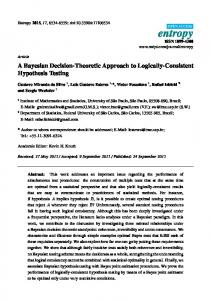
Fig. 5. Cost utility functions used to express the stakeholder perceptions.
Fig. 6. Expected value of the cost utility as a function of different rainfall threshold values. This analysis is repeated for each time rainfall accumulation time T and for each Antecedent Soil Moisture conditions class. For instance this graph is referred to AMC II and T=12 h.
2.3
Step 2: Fitting the joint probability density function
Once the corresponding pairs of values (the rainfall total and the relevant maximum water stage or discharge) have been sorted into the three AMC classes, for each class one can use these values to determine the joint probability density functions (jpdf) between the rainfall total and the relevant maximum discharge (or the water stage), to be used in step three. A jpdf will be estimated for each different forecasting horizon T , which will coincide with the rainfall accumulation time. The problem of fitting a bi-variate density f (q, v |T ) in which marginal densities are vastly different (quasi lognormal for that of discharges and quasi exponential in terms Hydrol. Earth Syst. Sci., 10, 413–426, 2006
Fig. 7. Example of the rainfall thresholds derived for each AMC class as a function of rainfall accumulation time: when the soil is wet the threshold will obviously be lower.
Fig. 8. Box plot of the mean monthly soil moisture condition calculated using the TOPKAPI model for the Sieve catchment.
of rainfall totals) can be overcome either by using a “copula” (Nelsen, 1999) or more interesting a Normal Quantile Transform (NQT) (Van der Waerten, 1952, 1953; Kelly and Krzysztofowicz, 1997). Figure 4 shows an example of the shape of one of the resulting bi-variate densities. 2.4
Step 3: Estimation of the most convenient rainfall threshold
The concept of flood warning thresholds takes its origins from the flood emergency management of large rivers, where the travel time is longer than the time required to implement the planned protection measures. In this case, the measurement of water stages at an upstream cross section can give accurate indications of what will happen at a downstream section in the following hours. Therefore, critical threshold levels were established in the past on the basis of water stage www.hydrol-earth-syst-sci.net/10/413/2006/
M. L. V. Martina et al.: Bayesian rainfall thresholds
419
Fig. 9. The AMC calendar for the antecedent soil moisture condition estimation.
measurements rather than on their forecasts. Unfortunately, when dealing with smaller catchments, the flood forecasting horizon is mostly limited by the concentration time of the basin, which means that one has to forecast the discharges and the river stages as a function of the measured or forecasted precipitation. In this case, uncertainty affects the forecasts and the problem of issuing an alert requires determining the expected value of some utility or loss function. In the present work, following Bayesian decision theory (Benjamin and Cornell, 1970; Berger, 1986), the concept of “convenience” is introduced as the minimum expected cost under uncertainty. The term “cost” does not refer to “actual costs” of flood damages that are probably impossible to be determined, but rather a Bayesian utility function describing the damage perception of the stakeholder, which may even include the non commensurable damages due to “missed alert”. Without loss of generality, in the present work the following cost function, graphically shown in Fig. 5, is expressed in terms of discharge: ( U (q, v|VT , T ) =
a ∗ 1+be−c(q−Q ) a0 C0 + 0 ∗ 1+b0 e−c (q−Q )
when v ≤ VT and no alert is issued when v > VT and an alert is issued
(1) with T the time of rainfall depth accumulation, v the forewww.hydrol-earth-syst-sci.net/10/413/2006/
casted volume and VT the rainfall threshold value, while a, b, c and a 0 , b0 , c0 are appropriate parameters. Due to the fact that the utility functions are only functional to the final objective of providing the decision makers with tools reflecting their risk perception, the shape of such functions, as well as the relevant parameter values, can be jointly assessed, by analysing the relevant effects on the decision process over past events. U (q, v |VT , T ) is the utility cost function, which if v≤VT expresses the perception of damages when no alert is issued (the dashed line in Fig. 5): no costs will occur if the discharge q will remain smaller than a critical value Q∗ , while damage costs will grow noticeably if the critical value is overtopped. On the contrary, if v¿VT it expresses the perception of damages when the alert is issued (the solid line in Fig. 5) a cost which will be inevitably paid to issue the alert (evacuation costs, operational cost including personnel, machinery etc.), and damage costs growing less significantly when the critical value Q∗ is overtopped and the flood occurs. As can be seen from Fig. 5, the utility function to be used will differ depending on the value of the cumulated rainfall forecast v and the rainfall threshold VT . If the forecast precipitation value is smaller or equal to the threshold value, the alert will not be issued; on the contrary, if the forecasted precipitation value Hydrol. Earth Syst. Sci., 10, 413–426, 2006
420
M. L. V. Martina et al.: Bayesian rainfall thresholds
Table 1. AMC classes definition according to the SCS approach
Table 2. Two-by-two contingency table for the assessment of a threshold based forecasting system
5-day antecedent rainfall totals [mm] AMC class AMC I (dry) AMC II (medium) AMC III (wet)
Dormant season
Growing season
P