Er (0.3,0.2,0.1,0,-0.1,-0.2,-0.3). DA (0.7). 2 inspectors. 3 inspectors. 4 inspectors. MtCh(2 Inspectors). MtCh(3 Inspectors). MtCh(4 Inspectors). 0. 0.2. 0.4. 0.6. 0.8.
A Bayesian Model for Controlling Software Inspections V. Gupta, A.R. Patnaik, N. Goel Cistel Technology Inc., 210 Colonnade Road, Suite 200, Ottawa, Ontario, Canada K2E 7L5. K. El Emam Institute for Information Technology, NRC, Montreal Road, Ottawa, Canada K1A OR6. C. H. Lung Department of Systems and Computer Engineering, Carleton University, Ottawa, Canada K1S 5B6. A. R. Nayak School of Information Technology and Engineering, University of Ottawa, Canada K1N 6N5.
Abstract We investigate both the objective and the subjective defect content estimation techniques (DCETs) for controlling software inspections. We performed extensive Monte Carlo simulations for the evaluation of these techniques under realistic software conditions. Capture-recapture (CR) models, the most popular objective DCETs, used in biology to estimate the size of animal population, have been proposed for the estimation of defects in the software artefact. The objective of the simulations was to find the best CR model. The results indicate that the CR models break down with sparse data. Due to the general failure of CR models under realistic conditions, we investigated an alternative approach: the use of subjective estimates of effectiveness by the inspectors for making the reinspection decision. In this study, we evaluated one of the Bayesian CR models, subjective DCETs, to estimate the defect content. Our results suggest that introducing the subjective estimate significantly improves the decision accuracy over the previously used CR models. 1 Introduction Inspection of software products is a cost-effective way to find defects for timely removal and to determine the quality level of working products immediately after their development (Gilb, 1993). Throughout the development phases of a software project, project managers need feedback on product quality to decide on appropriate further development and quality assurance activities. Michael Fagan first described software inspections in 1976 (Fagan, 1976). Since then there have been many variations and experiences described (Peterson et al. 2002). A typical inspection involves a team of three to five people examining and understanding a document to find defects. It has been shown that software inspection can lead to the detection and correction of anywhere between 50 and 90 percent of the defects in a software artefact (Fagan 1986, Briand et al. 1998). The industrial experience indicating a 30 times return on investment for every hour devoted to inspection of software require ment specifications has been reported by Doolan (Doolan 1992). Russell reports a similar return of 33 hours of maintenance saved for every hour of inspection invested (Russell 1991). The magnitude of this benefit depends primarily on the quality of the inspection. Contemporary research has focused on improved reading techniques and on reinspections for increasing the effectiveness of inspections (Emam and Laitenberger, 2001). Our focus in this paper is on the later. Reinspections can be considered a part of the general problem of when to stop inspections. The decision of whether to reinspect, further depends on a good estimation of the number of defects in the software artefact. In the recent past, there has been an increase of research activity in developing and improving defect content estimation techniques (DCETs) for software inspections. All of these techniques use quantitative models for estimating the number of defects in a software document from data collected after a software inspection has been carried out. The logic behind applying DCETs is that by estimating the number of defects in a document, the remaining defects can be calculated, and subsequently an objective decision can be made on whether to reinspect the software document or let it pass to the next phase. In this manner, the document quality (defined in terms of defect density) and the inspection process quality (defined in terms of its effectiveness) can be controlled.
Six commonly used CR models were evaluated to estimate the population size (Briand et al. 2000, Emam and Laitenberger, 2001). These authors used mixed set of defects. Using 6 inspectors and actual inspection data Briand et al. concluded that a minimum of 4 inspectors to be used in CR models. They also reported that the models Mh and Jackknife perform better than the other models. Emam and Laitenberger on the other hand used Monte Carlo simulations and two inspectors and a set of mixed type of defects. These authors find that though none of the six models performed satisfactorily, the model MtCh performed the best with respect to failures and decision accuracy. Gupta et al. (2003) extended the work of Emam and Laitenberger (2001) under realistic conditions. A realistic scenario includes few hard (major) defects and few inspectors. While it is relatively simpler to find and correct minor defects, the major defects, though their number is small, remain largely undetected and cause potentially the most serious damage. Their aim was to estimate the population of difficult defects. This paper concludes that the model MtCh performs better than the rest of the models. However, the models tend to perform poorly when the data are sparse. The accuracy of the models can be improved by adding more information. Specifically, three promising avenues can be considered. The first avenue is to improve on the objective data, e.g., by adding metrics such as the size of the module under inspection and effort to the models. The limitations associated with these two parameters are: firstly, it is hard to get people to accurately collect objective data consistently and secondly, the size depends on the type of artefact. We would need a different model for each artefact. The second avenue is to look into subjective data. Subjective estimates depend on the knowledge and capability of the individual inspector, who inspects the object carefully and reports the defects. The basic concept behind the subjective estimates is to ask inspectors after an inspection to estimate the percentage of defects in a document they believe they have actually found (Emam et al. 1999). Combining this information with a control data in a Bayesian DCET, one can estimate the total number of defects in a document. There is evidence that subjective estimates by professional inspectors of their personal effectiveness can be very accurate. This approach is appealing because it requires the estimate from the most experienced inspector, therefore is applicable irrespective of the total number of inspectors in the team. Also, it does not require significant changes to an existing inspection implementation such as collecting more detailed data on defects, nor any extra effort for inspection participants. Therefore, we decided to take this approach. The third avenue is to use models that use estimation techniques particularly suited to small data sets, for e.g., used to estimate the size of endangered species. We strongly recommend this approach for future work. The motivation for investigating the subjective estimates of effectiveness comes from the earlier work of Emam et al. (1999). In a study comparing code reading, functional testing, and structural testing, it was noted that readers could estimate quite accurately their own effectiveness. In the CR models, we only considered the capability of the inspectors in an objective manner and not their experience, which is a subjective quantity. In software inspection, often the inspectors can, to some degree of certainty based on their experience, predict the percentage of defects found by them after the inspection process. This prior information can be used in capture-recapture to formulate Bayesian models. In fact, Bayesian techniques are applied in wildlife studies. However, so far, such techniques have not been applied to software engineering studies. We decided to apply the Bayesian techniques for the first time, to estimate the defect population from the inspected data. In this paper, we show how subjective estimates of effectiveness can be applied to making the reinspection decision for code documents. In section 2, we discuss the Bayesian technique used in the software engineering context. Section 3 gives the overview of the research method and the evaluation criteria. In section 4, we present the results and section 5 discusses the results in detail. Finally, the conclusion of the research and the scope for future work are given in section 6. 2 Background We consider the problem of estimating the size of the closed population based on the results of certain type mark-resighting sampling design. In many cases of population studies, prior information is available about the population size. We have incorporated the prior information using a beta distribution and derived Bayesian estimators for the population size. 2.1 Multiple mark resighting model in software engineering context and Bayesian inference We follow the Bayesian model as described by Ananda (1997) used to estimate the population of mountain sheep. In software engineering context, the defects correspond to the animals and each trapping corresponds to an independent inspection done by an inspector.
Let N be the total number of defects in the software, n 0 be the number of defects found by the most experienced inspector from the inspection team, s be the number of inspectors, ni ( i=1,…,s-1) be the number of defects found by each inspector and
mi
(I=1,…,s-1) are the number of defects found by each inspector that overlapped with the most experienced inspector (these are the subset of n0 defects). These sample sizes ni are assumed to be coming from a density φ λ (n) , where λ is an unknown
mi given ni follows the hypergeometric distribution. When ni values are small and n0 is large, this distribution can be approximated by the binomial distribution with parameters n 0 and p = n 0 / N , parameter. The distribution of
As the second stage samples are independent, the likelihood function
L ( p, λ ) =
∏
s −1 i =1
L( p, λ ) can be written as
ni mi p (1 − p) ni − mi φ λ (n) mi
Eq 1
and the maximum likelihood estimate of population size N is given by
Nˆ = n0 (∑ n i ) / (∑ mi )
Eq 2
which is called the Lincoln-Peterson estimator. In the Bayesian method, the maximum likelihood function is modified by the prior distribution to give the posterior density. The prior distribution is described by a beta density with parameters a and b. Using this modified function the Bayesian estimate of the population size N is given by s −1 Nˆ ab = n0 a + b + ∑ ni − 1 i= 1
s −1 a + ∑ mi − 1 i =1
Eq 3
In case of no prior information for the estimation, then a uniform prior on p corresponding to the choice (a=1, b=1) or a generalized prior density on p with a choice such as (a=1, b=0) can be taken. With the second choice, the generalized Bayesian estimate of the population size will be the same as the maximum liklelihood estimate. The approach we have taken for our research involves the estimation of the prior parameters a and b using the available prior data. With the prior data, given mean E(p) and standard deviationσ p , the prior parameters a and b were evaluated by using the formula E(p) = a / (a + b), and
σ p2 = ab(a + b + 1) -1 (a+b) –2
Eq 4
2.2 The use of subjective estimates in software engineering context The subjective DCET, as used in this paper, uses the prior knowledge of the most experienced inspector involved in the inspection process. The prior information or the subjective estimate is based on an individual inspector’s perception of the percentage of defects in a document that s/he has found. This estimate is produced after reading the document and logging the defects. The subjective estimate is affected by many different factors such as the particular reading technique used by the inspectors (Laitenberger et al. 1999), the degree of difficulty of the defects as well as the experience of the inspectors (Gupta et al. 2003). 3 Research Method In this section we specify the study points for our simulation, and describe the methodology used for the evaluation of the subjective DCET.
3.1 Study Points Three sets of variables were considered for the simulations: the number of hard type of defects, the probability of a defect being found, and the inspector capability. We performed Monte Carlo simulations with the population size of 10, 20 and 30 defects with detection probabilities of 0.1 (very difficult to detect) and 0.4 (moderately difficult). We used 2, 3 and 4 inspectors for the simulations. These parameters resemble what one would expect to see in a real inspection. Inspectors 2 3
Ability to detect defects (0.1, 0.9), (0.25, 0.75), (0.4,0.6), (0.3, 0.3), (0.8, 0.8), (0.5, 0.5) (0.1, 0.5, 0.9), (0.25, 0.5, 0.75), (0.4, 0.5, 0.6), (0.3, 0.5, 0.3), (0.8,0.5,0.8), (0.5, 0.5, 0.5) (0.1,0.4,0.6,0.9), (0.1,0.1,0.9,0.9), (0.5,0.5,0.9,0.9), (0.9,0.9,0.9,0.9), (0.1,0.1,0.1,0.1), (0.5,0.5,0.5,0.5), (0.5,0.5,0.5,0.9), (0.1,0.5,0.5,0.5), (0.1,0.1,0.1,0.9), (0.1,0.9,0.9,0.9)
4 Table 1 Numbers within the brackets indicate the ability of an inspector to detect a defect for each inspection. For example, (0.9,0.9,0.9,0.9) is a team of four experts, while (0.1,0.1,0.1,0.1) is a team of four novices. For each study point, defined as a combination of inspector ability, defect population size and defect difficulty, 1000 inspections were simulated. 3.2 Capture-recapture data matrix The basic capture data we obtain after an inspection can be conveniently expressed in the form of a data matrix where, for each defect one must note all the inspectors who detected this defect. Assuming that we denote the total (and unknown) number of defects as N and the number of inspectors involved in the estimation procedure as k we can obtain the capture-recapture data matrix in the following manner:
x .11 x 21 X = . x N1
x 12
....
x 22
.....
.
.....
xN2
......
x1 K x2K . x Nk
X ij = 1 if inspector i detected defect j = 0 if undetected 3.3 Selection of Bayesian parameters The prior distribution is critical to the Bayesian method. This distribution is described by a and b parameters which are determined by the prior mean E(p) and the standard deviation σ p . In our simulations we select σ p and E(p) in the following manner. Since we do not have any knowledge of the prior, we try to determine these parameters from the data matrix described above. We define the mean as n0 / N . We allow for the fact that our estimated number can deviate as much as upto
± 30 %.
Thus the prior mean can now be written as
E ( p) = where
Er = 0, ± 0.1, ± 0.2, ± 0.3.
n0 N − Er × N
Eq 5
We chose values of 0.025, 0.05, 0.075, 0.1 and 0.2 for standard deviation. For each value of standard deviation, we had seven values of E(p) as given above. 3.4 Evaluation Criteria We evaluated the performance of the model under the following three criteria. 1.
The central tendency of the accuracy of the estimator. This was used to describe the average performance of the estimator. 2. The failure rate of the model. 3. The decision accuracy of the model. For controlling inspections, this decision was based on whether the effectiveness of the inspection is above a specified threshold. The above mentioned criteria are explained in detail below. 3.4.1 Decision Accuracy We are using DCETs for making a binary reinspection decision. For controlling inspections, this decision would be based on whether the effectiveness of the inspection is above a specified threshold. The effectiveness threshold is set to achieve a high quality inspection that ensures that the most detectable defects have been detected in the software artefact. Since we do not know the actual effectiveness, we use the model’s estimate to calculate the estimated effectiveness. Let Qp denote the threshold effectiveness set by the organization, then the decision can be stated in terms of the following inequality:
Qp ≤
where
D ˆ N ab
D denotes the total number of unique defects found by the inspection team and
Eq 6
D is the estimated inspection Nˆ ab
effectiveness. The artefact is passed on to the next phase if this inequality is satisfied. If it is not satisfied, then the artefact should be reinspected. We used the same two values of thresholds, 0.57 and 0.7 for our simulations as was used by Emam and Laitenberger (2001). The lower threshold is intended to ensure “above average” defect detection effectiveness, and the higher threshold is intended to ensure “best in class” effectiveness. 4 Results The primary aim of this research was to evaluate the Bayesian method of estimating the population of defects in a piece of software. In this method we use the subjective estimate (i.e. prior) of the most experienced inspector. As mentioned earlier, we have four main variables for our simulations: number of inspectors and their abilities, number of defects and their degree of difficulty. We observe that the decision accuracy (DA) decreases as the standard deviation of the prior increases. We also note that within a given standard deviation, the DA does not seem to change significantly. It was also observed that the failure rate in each simulation increases when the abilities of the inspectors decrease and also when the defects become more difficult to find. These three general trends are observed for the entire simulations. 1.
We first considered changing the number of inspectors while keeping all the other parameters fixed. The results for 10, 20 and 30 defects and the degree of difficulty of 0.1 and standard deviation of 0.025 are shown in Tables 2a, b and c. The DA for both the thresholds (0.57 and 0.7) increases as the number of inspector increases. Here we chose the inspector abilities as 0.5 for all the inspectors, which is a moderate ability. The DA of 10 defects increases from 0.62 to 0.87 for a threshold of 0.7 as the number of inspectors increase from 2 to 4. There is a similar increase in DA for a threshold of 0.57. This trend is observed for 20 and 30 defects as well.
2.
We obtain the second set of results by varying the ability of the inspectors. In Table 3, we show the DA for a case of 4 inspectors and 20 defects. The two groups of inspectors have been chosen to illustrate the extreme variations
i.e. a team of 4 experts and a team of 4 novices. The DA for the team of experts is significantly more than the DA of a team of novices, for both the thresholds used in our simulations. 3.
Next, we vary the number of defects while not changing the number and the ability of the inspectors. Table 4a, b and c show the results of DA for 2, 3 and 4 inspectors respectively. The DA increases with increasing number of defects for a given number of inspectors. For example, the DA increases from 0.63 to 0.96 for a threshold of 0.7. Similar increase in DA is observed for 0.57 threshold as well. The same trend is observed for all the inspection teams.
Er 0.3 0.2 0.1 0 -0.1 -0.2 -0.3
2 Inspectors DA(.7) DA(.57) 0.62 0.62 0.66 0.66 0.64 0.64 0.65 0.65 0.60 0.60 0.64 0.64 0.66 0.66
3 Inspectors DA(.7) DA(.57) 0.76 0.73 0.79 0.78 0.79 0.79 0.78 0.78 0.79 0.79 0.81 0.81 0.79 0.79
4 Inspectors DA(.7) DA(.57) 0.87 0.78 0.86 0.84 0.86 0.86 0.87 0.87 0.87 0.87 0.88 0.87 0.86 0.86
Table 2a: 10 Defects of .1 degree of difficulty and standard deviation of 0.025 Er 0.3 0.2 0.1 0 -0.1 -0.2 -0.3
2 Inspectors DA(.7) DA(.57) 0.88 0.88 0.86 0.86 0.89 0.89 0.88 0.88 0.87 0.87 0.86 0.86 0.87 0.87
3 Inspectors DA(.7) DA(.57) 0.94 0.94 0.95 0.95 0.96 0.96 0.95 0.95 0.95 0.95 0.96 0.96 0.95 0.95
4 Inspectors DA(.7) DA(.57) 0.98 0.96 0.98 0.98 0.99 0.99 0.99 0.99 0.99 0.99 0.99 0.99 0.98 0.98
Table 2b: 20 Defects of .1 degree of difficulty and standard deviation of 0.025
Er 0.3 0.2 0.1 0 -0.1 -0.2
2 Inspectors DA(.7) DA(.57) 0.95 0.95 0.94 0.94 0.94 0.94 0.94 0.94 0.96 0.96 0.96 0.96
3 Inspectors DA(.7) DA(.57) 0.99 0.99 0.99 0.99 0.99 0.99 0.99 0.99 1.0 1.0 0.99 0.99
4 Inspectors DA(.7) DA(.57) 0.99 0.99 0.99 0.99 0.99 0.99 1.0 1.0 0.99 0.99 0.99 0.99
-0.3
0.96
0.99
0.99
0.96
0.99
0.99
Table 2c: 30 Defects of .1 degree of difficulty and standard deviation of 0.025
Er
0.3 0.2 0.1 0 -0.1 -0.2 -0.3
4 Inspectors abilities (experts) (0.9,0.9,0.9,0.9) DA(.7) DA(.57) .93 .74 .99 .94 1.0 0.98 1.0 1.0 1.0 0.99 1.0 0.99 1.0 0.99
4 Inspectors abilities (novices) (0.1, 0.1, 0.1, 0.1) DA(.7) DA(.57) 0.55 0.55 0.55 0.55 0.53 0.53 0.56 0.56 0.57 0.57 0.58 0.58 0.53 0.53
Table 3: 20 Defects of .1 degree of difficulty and standard deviation of 0.025
Er 0.3 0.2 0.1 0 -0.1 -0.2 -0.3
10 defects DA(.7) DA(.57) 0.63 0.62 0.64 0.63 0.65 0.65 0.64 0.64 0.64 0.64 0.62 0.62 0.63 0.63
20 defects DA(.7) DA(.57) 0.86 0.86 0.88 0.88 0.86 0.86 0.85 0.85 0.87 0.87 0.88 0.88 0.86 0.86
30 defects DA(.7) DA(.57) 0.96 0.96 0.96 0.96 0.96 0.96 0.96 0.96 0.95 0.95 0.96 0.96 0.95 0.95
Table 4a: 2 Inspectors with .1 degree of difficulty and standard deviation of 0.025
Er 0.3 0.2 0.1 0 -0.1 -0.2 -0.3
10 defects DA(.7) DA(.57) 0.78 0.76 0.78 0.78 0.79 0.79 0.79 0.79 0.80 0.80 0.78 0.78 0.77 0.77
20 defects DA(.7) DA(.57) 0.96 0.95 0.96 0.96 0.96 0.96 0.96 0.96 0.96 0.96 0.96 0.96 0.95 0.95
30 defects DA(.7) DA(.57) 0.99 0.99 0.99 0.99 0.99 0.99 0.99 0.99 1.0 1.0 0.99 0.99 0.99 0.99
Table 4b: 3 Inspectors with .1 degree of difficulty and standard deviation of 0.025
Er
10 defects DA(.7) DA(.57)
0.3 0.2 0.1 0 -0.1 -0.2 -0.3
0.87 0.89 0.87 0.87 0.86 0.86 0.86
0.80 0.87 0.87 0.87 0.85 0.86 0.86
20 defects DA(. DA(.57) 7) 0.99 0.96 0.98 0.98 0.98 0.98 0.98 0.98 0.99 0.99 0.99 0.99 0.99 0.99
30 defects DA(.7) DA(.57) 1.0 1.0 1.0 1.0 1.0 1.0 1.0
1.0 1.0 1.0 1.0 1.0 1.0 1.0
Table 4c: 4 Inspectors with .1 degree of difficulty and standard deviation of 0.025 5 Discussion We can understand the results and the behaviour of the Bayesian model in terms of the data matrix and the prior. The product of the ability of the inspectors and the number of defects and their degree of difficulty determine the sparseness of the data matrix. The estimated population depends on the values of n 0 , m1, n1 and a and b parameters of the beta distribution (see Eq 3). The parameter m1 determines the overlap of defects found by more than one inspector. It is clear from Eq 3 that if m1=0 (happens when data matrix is sparse), the estimated population depends more on a and b values, and hence the prior mean E(p) and standard deviation σ p . On the other hand when the data matrix is filled (happens when the ability of the inspectors is high and the defects are easier to find, as well as the defects being more in number) the estimated population depends more on overlap parameter m1 and n1. Therefore, in the case of a sparse data matrix, the estimated population depends entirely on the prior mean and standard deviation, hence it is very important to have an accurate value of the prior. This can be achieved with a team of experts as was shown earlier. However, if the prior happens to be significantly off the actual value, then it is likely that the estimated population would be equally inaccurate as well. The failure to estimate the population occurs when the data matrix is completely empty. This happens when the team consists of novices and the degree of difficulty of the defects is high. Given the above explanation of the data matrix we can easily understand all the results of the Bayesian model. The data matrix is sparse for low number of defects and gets filled with large number of defects as well as larger number of inspectors, thereby increasing the DA. Prior research has identified a specific CR model, model MtCh, as the most appropriate for inspections (Briand et al. 2000, Emam and Laitenberger 2001, Gupta et al. 2003). Next we compare the Bayesian results with the model MtCh obtained earlier. Figures 1 and 2 show the DA (0.7 and 0.57 respectively) as a function of Er for 2,3 and 4 inspectors for both Bayesian and MtCh models for 10 defects and 0.1 degree of difficulty. In each case the Bayesian results are much better than MtCh. Under all the circumstances the DA values of Bayesian are remarkably high than that of MtCh. Since Er parameter was fixed for MtCh, we have the same value of DA plotted for all values of Er. Though we have shown the graphs for σ p =0.025, the result is same for other values of σ p . Even 4-inspector MtCh is much less than 2, 3-inspector Bayesian. 6 Conclusion and Future Prospects In this paper we have applied a Bayesian technique to estimate the population of defects in the software engineering context. The results are extremely encouraging, particularly with respect to sparse data. Addition of subjective estimate improves the DA over the objective DCETs. The most critical parameter in Bayesian technique is the prior mean. In this respect it is extremely important to obtain the prior as accurately as possible. Having one expert in the team of inspectors helps more than having a large number of novices. There are other Bayesian estimation techniques but they differ in sampling methods (Basu and Ebrahimi 1998).
DA (0.7)
1 0.8
2 inspectors
0.6
3 inspectors 4 inspectors MtCh(2 Inspectors)
0.4 0.2 0 1
2
3
4
5
6
7
MtCh(3 Inspectors) MtCh(4 Inspectors)
Er (0.3,0.2,0.1,0,-0.1,-0.2,-0.3)
Fig 1: Comparison of DA of 0.7 for Bayesian and MtCh for 10 defects
DA (.57)
1 0.8
2 inspectors
0.6
3 inspectors
0.4
4 Inspectors
0.2
MtCh(2 Inspectors) MtCh(3 Inspectors)
0 1
2
3
4
5
6
7
MtCh(4 Inspectors)
Er (0.3,0.2,0.1,0,-0.1,-0.2,-0.3)
Fig 2: Comparison of DA of 0.57 for Bayesian and MtCh for 10 defects References Ananda, M. M. A., “Bayesian Methods for Mark-Resighting Surveys”, Communications in Statistics - Theory and Methods, 26(3), 685 - 697 (1997). Basu, S., Ebrahimi, N., "Estimating the number of undetected errors: Bayesian model selection", Division of Statistics, Northern Illinois University. Ninth International Symposium on Software Reliability Engineering, 4-7 Nov 1998. Briand, L., Freimut, B., Laitenberger, O., Ruhe, G., and Klein, B., “Quality Assurance Technologies for the EURO Conversion – Industrial Experience at Allianz Life Assurance”, In Proc. of Quality Week Europe, 1998. Briand, L., El Emam, K. and Freimut, B., “A Comprehensive Evaluation of Capture-Recapture Models for Estimating Software Defect Content”, IEEE Transactions on Software Engineering, 26(6):518-540, 2000. Doolan, E.P., “Experience with Fagan’s Inspection Method ,” Software-Preactice and Experience, vol. 22(2), pp. 173-182. , Feb 1992. Emam, Khaled. El., Laitenberger, O. and Harbich, T, “The Application of Subjective Estimates of Effectiveness to Controlling Software Inspections”, Technical Report, NRC/ERB-1060, 36 pages, NRC 43604, October 1999. Emam, K.El and Laitenberger, O., “Evaluating Capture-Recapture Models with Two Inspectors,” IEEE Thransactions on Software Engineering, vol 27, Sep 2001. Fagan, M.E., “Design and Code Inspections to Reduce Errors in Program Development,” IBM Systems Journal, 15(3): 182- 211,1976.
Fagan, M. E., “Advances in Software Inspections”, IEEE Transaction on Software Engineering, 12(7): 744-751, 1986. Gilb, T. and Graham, D., “Software Inspection”, Addison-Wesley Publishing Company, 1993. Gupta, V., Patnaik, A. R., Emam, K. El. and Goel, N., “System for Controlling Software Inspection”, CCECE 2003 Canadian Conference on Electrical and Computer Engineering, May 2003. Petersson, H., Thelin, T., Runeson, P. and Wohlin, C., “Capture-Recapture in Software Inspections after 10 Years Research – Theory, Evaluation and Application”, to appear in Journal of Systems and Software, 69(1), 2004. Russell, G.W., “Experience with Inspections in Ultralarge-Scale Developments,” IEEE Software, vol 8, pp. 25-31, 1991.