a bayesian network integration framework for modeling biomedical data

KATHOLIEKE UNIVERSITEIT LEUVEN FACULTEIT INGENIEURSWETENSCHAPPEN DEPARTEMENT ELEKTROTECHNIEK Kasteelpark Arenberg 10, B-3001 Leuven (Heverlee)

A BAYESIAN NETWORK INTEGRATION FRAMEWORK FOR MODELING BIOMEDICAL DATA

Promotoren: Prof. dr. ir. Bart De Moor Prof. dr. dr. Dirk Timmerman

Proefschrift voorgedragen tot het behalen van het doctoraat in de ingenieurswetenschappen door Olivier GEVAERT

December 2008

KATHOLIEKE UNIVERSITEIT LEUVEN FACULTEIT INGENIEURSWETENSCHAPPEN DEPARTEMENT ELEKTROTECHNIEK Kasteelpark Arenberg 10, B-3001 Leuven (Heverlee)

A BAYESIAN NETWORK INTEGRATION FRAMEWORK FOR MODELING BIOMEDICAL DATA

Jury: Prof. dr. ir. Yves Willems, voorzitter Prof. dr. ir. Bart De Moor, promotor Prof. dr. dr. Dirk Timmerman, promotor Prof. dr. ir. Yves Moreau Prof. dr. ir. Johan Suykens Prof. dr. Mia Hubert Prof. dr. dr. Karin Haustermans Prof. dr. Peter J. van der Spek (Erasmus MC, Rotterdam)

U.D.C. 681.3*J3

December 2008

Proefschrift voorgedragen tot het behalen van het doctoraat in de ingenieurswetenschappen door Olivier GEVAERT

c

Katholieke Universiteit Leuven – Faculteit Ingenieurswetenschappen Arenbergkasteel, B-3001 Heverlee (Belgium) Alle rechten voorbehouden. Niets uit deze uitgave mag vermenigvuldigd en/of openbaar gemaakt worden door middel van druk, fotocopie, microfilm, elektronisch of op welke andere wijze ook zonder voorafgaande schriftelijke toestemming van de uitgever. All rights reserved. No part of the publication may be reproduced in any form by print, photoprint, microfilm or any other means without written permission from the publisher. ISBN 978-94-6018-001-9 U.D.C. 681.3*J3 D/2008/7515/110

Dankwoord Toen ik in 2004 op zoek was naar een thesisonderwerp kwam ik in contact met Prof. Bart De Moor. Na enkele mailtjes kwam ik uiteindelijk op zijn bureau waar ik slechts enkele woorden stamelde: ”Euh, ja.”. Enkele weken later gaf Bart mij het vertrouwen en mocht ik een doctoraat starten in de bioinformatica groep binnen Sista. Bedankt, Bart voor de kansen die je mij gegeven hebt en het continue enthousiasme waarmee je mij hebt ge¨ınspireerd! Ik kwam al snel in contact met mijn huidige co-promotor Prof. Dirk Timmerman. Hij introduceerde mij in het klinische onderzoek in de gynaecologische oncologie en bracht mij in contact met vele clinici. Bedankt voor alles Dirk, jij was de katalysator voor ontelbare projecten. Vervolgens wil ik mijn begeleidingscommissie, Prof. Johan Suykens, Prof. Yves Moreau en Prof. Mia Hubert, bedanken voor het kritisch evalueren van mijn onderzoek en doctoraatstekst. Bovendien wil ik ook Prof. Yves Willems, bedanken voor de bereidheid om mijn jury voor te zitten. Verder wil ik Prof. Karin Haustermans bedanken voor de super interessante samenwerking op een heel uitdagende data set. Bedankt dat je in mijn jury wil zetelen en bedankt voor alle steun. Tenslotte wil ik Prof. Peter van der Spek bedanken om deel uit te maken van mijn doctoraatsjury. Bedankt Peter voor de samenwerking die ontstaan is op familie- en trouwfeesten. Ik had nooit gedacht over bioinformatica te babbelen op deze familiegelegenheden en hier is een heel fijne samenwerking uit voortgevloeid met Andrew en Pim. Natuurlijk wil ik ook zowel de voormalige als huidige collega’s van SISTA bedanken: Nathalie, Gert, Kathleen, Kristof, Ruth, Pieter, Qizheng, Joke, Steven, Bert C, Bert P, Frizo, Peter V, Tom, Raf, Wout, Shi, Tim, Karen, Thomas, Anneleen, Niels, Fabian, Riet, Léo, Liesbeth, Lieven, Peter K, Sonia, Daniela, Tunde, Ernesto, Peter C en Jiqiu voor de fijne sfeer, koffiepauzes, discussies en sofa-momenten. Verder ben ik veel dank verschuldigd aan Frank De Smet. Bedankt Frank dat je me binnengeloodst hebt in de wondere wereld van de bioinformatica en microarrays. Je hebt een grote invloed gehad op mijn onderzoek en zonder jou had het mischien helemaal anders uitgedraaid. Bedankt ook voor het kritisch nalezen, niet alleen van mijn thesis maar van al mijn manuscripten! Verder wil ik de IT en website specialisten bedanken: Kris en Maarten zonder jullie i

ii hulp zouden we heel veel tijd moeten investeren om de juiste ICT keuzes te maken. Ida, Ilse en Mimi bedankt voor de administratieve en financiële assistentie. Geen enkele thesis komt tot stand zonder samenwerkingen, zeker in het multidisciplinaire bioinformatica domein. Ik moet dan ook veel mensen bedanken voor de fijne samenwerking: Prof. Ignace Vergote, Toon en Isabelle voor de microarray en proteomics projecten op ovarium en andere tumoren. Caroline voor jouw niet te onderschatten bijdrage aan het IOTA data set. Prof. Tom Bourne, Dr. Emma Kirk and Prof. George Condous for the nice collaboration on pregnancies of unknown location. Karin L, Prof. Legius en Eline voor de oude en nieuwe samenwerkingen op arrayCGH data. Prof. Sabine van Huffel en de Biomed studenten onder haar begeleiding: Ben, Vanya en Lieven. Prof. Etienne Waelkens voor de soms hilarische vergaderingen en zeker voor de expertise in alle proteomics projecten. Prof. Sabine Tejpar, Annelies, Wendy en Bart voor de oude en nieuwe samenwerkingen. Andrew for the nice collaboration with the Rotterdam bioinformatics group en Pim voor de samenwerking rond hersentumoren. Prof. Thomas D’Hooghe, Kyama, Attila en Amelie voor de fijne samenwerking rond endometriose. Ann voor de toffe samenwerking rond borsttumoren. Tenslotte, de hepatologie onderzoekers Prof. Jos van Pelt, Prof. Chris Verslype, Hannah en Louis. Verder wil ik ook Jacqueline bedanken voor alle tijd die je hebt ge¨ınvesteerd om mijn tekst na te lezen. Hier wil ik ook graag mijn ouders bedanken voor de kansen die ze mij hebben gegeven om hier te geraken, en mijn familie, kleine zus Julie, Tom, grote zus Gretel, Dan, mijn petekind Hanne en Jutta. Tenslotte, Leen bedankt om in mij te geloven, mijn vele uiteenzettingen over mijn onderzoek te aanhoren en de bereidheid om misschien binnenkort andere horizonten te verkennen. Olivier

Leuven 8 december 2008

Abstract In the past decade microarray technology has had a big impact on cancer research. More recently other technologies such as mass spectrometry-based proteomics or array comparative genomic hybridization have emerged as data providers with potentially similar impact. These technologies have a top-down approach in common instead of a bottom-up. Whether it is the genome, transcriptome or proteome that is targeted, each technology attempts to capture its corresponding ‘omics’ as a whole. Moreover, the data resulting from these technologies potentially hold information on the actual biological reasons why subsets of tumors behave differently, instead of relying on general clinical data or morphological characteristics of a tumor. In our research, we investigated how omics data can be used to predict diagnosis, prognosis or therapy response in cancer. The large dimensionality of omics data however prohibits direct interpretation and requires dedicated models. Biomedical decision support modeling attempts to tackle this issue and aims to build reliable models. We focused on the use of Bayesian networks as biomedical decision support model. More specifically, we developed a Bayesian network integration framework able to integrate heterogeneous and high-dimensional data. We consider two specific types of data in our framework: patient specific data or entity specific data. We define patient specific data as primary data and entity specific data as secondary data. The latter characterizes entities within each omics layer such as genes in the genome, mRNA in the transcriptome or proteins in the proteome. First, we illustrate Bayesian network modeling on two primary data sources separately: clinical and genomic data. Secondly, we develop algorithms to integrate primary data sources. Finally, we extend the framework to include secondary data sources. Besides the use of publicly available data and due to the availability of unique data gathered at the University Hospitals Leuven, we applied our framework on two main cancer sites: ovarian cancer and rectal cancer. Our results show the potential of integrating both primary and secondary data sources. Finally, we look into the future and project which research avenues should be pursued to improve the framework.

iii

iv

Korte Inhoud Microroostertechnologie heeft een grote impact gehad op het kankeronderzoek in het laatste decennium. Recent zijn ook andere technologieën zoals proteomica gebaseerd op massa spectrometrie en microroostertechnologie voor comparatieve genomische hybridisatie opgedoken als data leveranciers met potentieel gelijkaardige impact. Deze technologieën hebben een “top-down” aanpak gemeenschappelijk waarbij het genoom, transcriptoom of proteoom in hun geheel onderzocht worden. Bovendien bevatten de “omics” data die geleverd worden door deze technologieën potentieel informatie betreffende de biologische kenmerken die verantwoordelijk zijn voor het gedrag van tumoren in plaats van klinische of morfologische karakteristieken. In ons onderzoek hebben we onderzocht hoe omics data gebruikt kunnen worden voor het voorspellen van de diagnose, prognose of therapierespons van kankerpatiënten. De hoge dimensionaliteit van omics data echter verhindert de directe interpretatie van deze data and vereist specifieke modelleringstechnieken. Biomedische besluitvormingssystemen hebben als doel om dit probleem aan te pakken en het gebruik hiervan is gericht op het bouwen van betrouwbare modellen ter ondersteuning van de behandeling van patiënten. Meer specifiek hebben we gebruik gemaakt van een Bayesiaans netwerk als besluitvormingsysteem. Hiervoor hebben we een raamwerk uitgebouwd voor de integratie van heterogene en hoog dimensionale data waarbij twee verschillende types data werden gemodelleerd: primaire en secundaire data. We definiëren primaire data als patiënt specifiek terwijl secundaire data specifiek zijn voor de entiteiten binnen elk omics dataset. Deze entiteiten zijn genen voor het genoom, mRNA voor het transcriptoom en prote¨ınen voor het proteoom. Ten eerste, hebben we het gebruik van Bayesiaanse netwerken ge¨ıllustreerd voor het modelleren van twee primaire databronnen: klinische en genomische data. Ten tweede, hebben we algoritmes ontwikkeld om primaire databronnen te integreren. Tenslotte, hebben we het raamwerk uitgebreid om ook secundaire databronnen te kunnen gebruiken. Naast het gebruik van publiek beschikbare data en ook door de aanwezigheid van unieke data verzameld in de Universitaire Ziekenhuizen Leuven, hebben we onze methodologie ook toegepast op data van ovarium- en darmkankerpatiënten. Onze resultaten tonen het potentieel aan van het integreren van primaire en secundaire databronnen. Tenslotte, kijken we naar de toekomst en vermelden we enkele uitdagingen om dit onderzoek voort te zetten.

v

vi

Acronyms ANN AUC BDIM BPIM BRCA CA125 CGH CNA CNG CNL CNV CPT CRT CT DNA EGFR ELISA ER FIGO HMM IDF IOTA LOO-CV LS-SVM MALDI-TOF MAP MCMC MRI mRNA pCR PI PPTC PR PRM

Artificial neural network Area under the ROC curve Best Decision Integration Model Best Partial Integration Model Breast cancer early onset gene Cancer antigen 125 Comparative genomic hybridization Copy number alteration Copy number gain Copy number loss Copy number variation Conditional probability table Chemo-radiation therapy Computed tomography Deoxyribonucleic acid Epidermal growth factor receptor Enzyme-linked immunosorbent assay Estrogen receptor Fédération Internationale de Gynécologie Obstétrique Hidden Markov model Inverse Document Frequency International ovarian tumor analysis consortium Leave one out cross validation Least squares support vector machine Matrix assisted laser desorption ionization time-of-flight Maximum a posteriori Markov chain monte carlo Magnetic resonance scan messenger RNA pathological complete response Pulsatility index Probability propagation in tree of cliques Progesteron receptor Probabilistic Relational Models

vii

viii PSV qRT-PCR RBF RCRG RI RMA RNA ROC SELDI-TOF SNP TAMXV TME TNM

Peak systolic velocity quantitative real time polymerase chain reaction Radial basis function Rectal cancer regression grade Resistance index robust multi-chip average Ribonucleic acid Receiver operator characteristic curve Surface enhanced laser desorption ionization time-of-flight Single nucleotide polymorphism Time-averaged maximum velocity Total mesorectal excision Tumor Node Metastases

Contents Dankwoord

i

Abstract

iii

Korte Inhoud

v

Acronyms

vii

Contents

ix

Nederlandse samenvatting 1

2

xiii

Introduction 1.1 Context . . . . . . . . . . . . . . . . . . . . . . . 1.2 Biomedical decision support . . . . . . . . . . . . 1.3 The omics revolution: technological breakthroughs 1.4 The molecular biology of cancer . . . . . . . . . . 1.5 Bayesian networks and Bayesian modeling . . . . 1.6 Objectives . . . . . . . . . . . . . . . . . . . . . . 1.7 Chapter-by-chapter overview . . . . . . . . . . . . 1.8 Specific contributions of this thesis . . . . . . . . . 1.9 Other research . . . . . . . . . . . . . . . . . . . .

. . . . . . . . .

. . . . . . . . .

. . . . . . . . .

. . . . . . . . .

. . . . . . . . .

. . . . . . . . .

. . . . . . . . .

. . . . . . . . .

. . . . . . . . .

. . . . . . . . .

1 1 2 4 7 10 11 13 14 15

A Bayesian network primer 2.1 Introduction . . . . . . . . . . . . . . . . . . . 2.2 Two paradigms for statistical inference . . . . . 2.3 Bayesian networks . . . . . . . . . . . . . . . 2.3.1 Definition . . . . . . . . . . . . . . . . 2.3.2 Bayesian network learning . . . . . . . 2.3.3 Priors . . . . . . . . . . . . . . . . . . 2.3.4 Inference . . . . . . . . . . . . . . . . 2.4 Evaluation measures . . . . . . . . . . . . . . 2.4.1 Receiver Operating Characteristic curve 2.4.2 Cross validation and randomization . . 2.5 Discretization . . . . . . . . . . . . . . . . . .

. . . . . . . . . . .

. . . . . . . . . . .

. . . . . . . . . . .

. . . . . . . . . . .

. . . . . . . . . . .

. . . . . . . . . . .

. . . . . . . . . . .

. . . . . . . . . . .

. . . . . . . . . . .

. . . . . . . . . . .

17 17 19 20 20 22 24 26 27 27 29 29

ix

. . . . . . . . . . .

. . . . . . . . . . .

x

Contents . . . .

. . . .

. . . .

. . . .

. . . .

. . . .

. . . .

. . . .

. . . .

. . . .

29 30 31 32

Ovarian and rectal cancer: background, aims and data. 3.1 Overview . . . . . . . . . . . . . . . . . . . . . . . 3.2 Ovarian cancer . . . . . . . . . . . . . . . . . . . . 3.2.1 Background . . . . . . . . . . . . . . . . . . 3.2.2 Previous research . . . . . . . . . . . . . . . 3.2.3 Aims for ovarian cancer decision support . . 3.3 Rectal cancer . . . . . . . . . . . . . . . . . . . . . 3.3.1 Background . . . . . . . . . . . . . . . . . . 3.3.2 Aims for rectal cancer decision support . . . 3.4 Publicly available data . . . . . . . . . . . . . . . . 3.4.1 van ’t Veer data set . . . . . . . . . . . . . . 3.4.2 Bild data . . . . . . . . . . . . . . . . . . .

. . . . . . . . . . .

. . . . . . . . . . .

. . . . . . . . . . .

. . . . . . . . . . .

. . . . . . . . . . .

. . . . . . . . . . .

. . . . . . . . . . .

. . . . . . . . . . .

. . . . . . . . . . .

33 34 34 34 37 41 41 41 42 44 44 46

Clinical data 4.1 Introduction . . . . . . . . . . . . . . . . . . . . . 4.2 Overview . . . . . . . . . . . . . . . . . . . . . . 4.3 Data . . . . . . . . . . . . . . . . . . . . . . . . . 4.4 Results . . . . . . . . . . . . . . . . . . . . . . . . 4.4.1 Predictive performance of BN1 . . . . . . 4.4.2 Markov blanket of outcome . . . . . . . . 4.4.3 Comparison with logistic regression models 4.5 Conclusions . . . . . . . . . . . . . . . . . . . . .

. . . . . . . .

. . . . . . . .

. . . . . . . .

. . . . . . . .

. . . . . . . .

. . . . . . . .

. . . . . . . .

. . . . . . . .

. . . . . . . .

47 47 48 49 50 51 52 55 55

Genomic data 5.1 Introduction . . . . . . . . . . . . . . . . . . . . . . . . . . 5.2 Aims and data . . . . . . . . . . . . . . . . . . . . . . . . . 5.3 Modeling . . . . . . . . . . . . . . . . . . . . . . . . . . . 5.3.1 Pooled analysis . . . . . . . . . . . . . . . . . . . . 5.3.2 Differential analysis . . . . . . . . . . . . . . . . . 5.3.3 Recurrent hidden Markov model . . . . . . . . . . . 5.3.4 Signature construction . . . . . . . . . . . . . . . . 5.3.5 Pathway enrichment analysis . . . . . . . . . . . . . 5.4 Results . . . . . . . . . . . . . . . . . . . . . . . . . . . . . 5.4.1 Identification of CNA . . . . . . . . . . . . . . . . . 5.4.2 Statistical analysis of CNA from differential analysis 5.4.3 Signature construction . . . . . . . . . . . . . . . . 5.4.4 Pathway enrichment analysis . . . . . . . . . . . . . 5.5 Conclusions . . . . . . . . . . . . . . . . . . . . . . . . . . 5.5.1 Previous work . . . . . . . . . . . . . . . . . . . . 5.5.2 Our results . . . . . . . . . . . . . . . . . . . . . .

. . . . . . . . . . . . . . . .

. . . . . . . . . . . . . . . .

. . . . . . . . . . . . . . . .

. . . . . . . . . . . . . . . .

. . . . . . . . . . . . . . . .

59 59 60 61 61 62 64 64 64 65 65 70 70 70 77 77 78

2.6 3

4

5

2.5.1 Motivation . . 2.5.2 Algorithms . . 2.5.3 Implementation Conclusions . . . . . .

. . . .

. . . .

. . . .

. . . .

. . . .

. . . .

. . . .

. . . .

. . . .

. . . .

. . . .

. . . .

. . . .

. . . .

. . . .

. . . . . . . .

Contents 6

7

8

xi

Integration of primary data sources 6.1 Introduction . . . . . . . . . . . . . . . . . . 6.2 Integration of clinical and microarray data . . 6.2.1 Data and model building . . . . . . . 6.2.2 Integration Methods . . . . . . . . . 6.2.3 Results . . . . . . . . . . . . . . . . 6.2.4 Discussion . . . . . . . . . . . . . . 6.3 Integration of microarray and proteomics data 6.3.1 Data preprocessing . . . . . . . . . . 6.3.2 Integration framework . . . . . . . . 6.3.3 Model evaluation . . . . . . . . . . . 6.3.4 Results . . . . . . . . . . . . . . . . 6.3.5 Discussion . . . . . . . . . . . . . . 6.4 Conclusions . . . . . . . . . . . . . . . . . .

. . . . . . . . . . . . .

. . . . . . . . . . . . .

. . . . . . . . . . . . .

. . . . . . . . . . . . .

. . . . . . . . . . . . .

. . . . . . . . . . . . .

. . . . . . . . . . . . .

. . . . . . . . . . . . .

. . . . . . . . . . . . .

. . . . . . . . . . . . .

. . . . . . . . . . . . .

. . . . . . . . . . . . .

81 . 81 . 83 . 83 . 83 . 85 . 87 . 89 . 92 . 92 . 93 . 94 . 99 . 101

Integration of secondary data sources 7.1 Introduction . . . . . . . . . . . . 7.2 Structure prior . . . . . . . . . . . 7.2.1 Gene prior . . . . . . . . 7.2.2 Outcome variable prior . . 7.3 Data . . . . . . . . . . . . . . . . 7.3.1 Model evaluation . . . . . 7.3.2 Discretization . . . . . . . 7.4 Results . . . . . . . . . . . . . . . 7.4.1 van ’t Veer data . . . . . . 7.4.2 Bild data . . . . . . . . . 7.5 Conclusions . . . . . . . . . . . .

. . . . . . . . . . .

. . . . . . . . . . .

. . . . . . . . . . .

. . . . . . . . . . .

. . . . . . . . . . .

. . . . . . . . . . .

. . . . . . . . . . .

. . . . . . . . . . .

. . . . . . . . . . .

. . . . . . . . . . .

. . . . . . . . . . .

. . . . . . . . . . .

. . . . . . . . . . .

Conclusions and Future Research 8.1 Conclusions . . . . . . . . . . . . . . . . . . . . . . . . . . . . . 8.2 Future research . . . . . . . . . . . . . . . . . . . . . . . . . . . 8.2.1 Extensions of the Bayesian network integration framework 8.2.2 The future of biomedical decision support . . . . . . . . .

. . . .

113 . 113 . 116 . 116 . 118

. . . . . . . . . . .

. . . . . . . . . . .

. . . . . . . . . . .

. . . . . . . . . . .

. . . . . . . . . . .

. . . . . . . . . . .

103 103 104 104 106 107 108 108 108 108 110 110

Bibliography

121

Publications by the author

137

Biography

143

xii

Contents

Data integratie met Bayesiaanse netwerken voor het modelleren van biomedische data Hoofdstuk 1: Inleiding Ovariumkanker vertegenwoordigt 4% van alle kwaadaardige aandoeningen bij vrouwen maar staat toch op de vijfde plaats als doodsoorzaak door kanker. Dit komt omdat deze aandoening in 80% van de gevallen in een te laat stadium ontdekt wordt (stadia III en IV) terwijl deze aandoening in het eerste stadium beter te behandelen is. De overleving na 5 jaar is 90% bij diagnose in stadium I, in latere stadia is dat slechts 35%. In de meeste gevallen wordt de aandoening pas ontdekt wanneer de tumor al is uitgezaaid en dan zijn de therapeutische mogelijkheden beperkt. De meerderheid van alle ovariale tumoren zijn goedaardig en kunnen behandeld worden met hormonale therapie of met een relatief eenvoudige chirurgische ingreep. De kwaadaardige tumoren zaaien echter uit en zijn levensbedreigend. De behandeling bestaat in veel gevallen uit majeure chirurgie door tussenkomst van een gynaecologische oncoloog. De adjuvante therapie bestaat uit het toedienen van chemotherapie. Helaas worden hierbij ook normale cellen aangetast met negatieve bijwerkingen tot gevolg. Biomedische besluitvormingssystemen hebben als doel om dit probleem aan te pakken en de clinicus te ondersteunen bij het nemen van beslissingen betreffende de behandeling van de patiënt. Dit gebeurt door het leren van een model gebaseerd op biomedische data waarvan de uitkomst gekend is. Dit model wordt vervolgens toegepast om de uitkomst te voorspellen van patiënten waarvoor de uitkomst gemaskeerd is. Enkele voorbeelden van zulke modellen zijn logistieke regressie, support vector machines en Bayesiaanse netwerken. Traditioneel werd voor het bouwen van medische besluitvormingssystemen vooral gebruik gemaakt van klinische data. Echter dankzij het humaan genoom project en technologische vooruitgang, werd een grote hoeveelheid moleculaire gegevens beschikbaar bijvoorbeeld de expressie van alle genen in het menselijk genoom. Door de hoge dimensionaliteit van deze data is het onmogelijk om deze data direct te interpreteren en is het een noodzaak geworden om medische besluitvormingssystemen te bouwen. In deze thesis hebben we ons tot doel gesteld om Bayesiaanse netwerken te gebruik xiii

xiv

Nederlandstalige samenvatting

om heterogene en hoog dimensionale data te modelleren in kankerpatiënten. Hiervoor hebben we een raamwerk uitgebouwd voor de integratie van twee verschillende types data: primaire en secundaire data. We definiëren primaire data als patiënt specifiek terwijl secundaire data specifiek zijn voor de entiteiten binnen elk omics dataset. Deze entiteiten zijn genen voor het genoom, mRNA voor het transcriptoom en prote¨ınen voor het proteoom. In Hoofdstuk 2 zijn we dieper ingegaan op de methodologie en in Hoofdstuk 3 hebben we de data die in deze thesis gebruikt werd nader toegelicht. Vervolgens, hebben we onze methodologie eerst toegepast voor het modelleren van twee afzonderlijke primaire databronnen: klinische data van ovariumkankerpatiënten in Hoofdstuk 4 en genomische data van ovariumkankerpatiënten met of zonder een mutatie in het BRCA1-gen in Hoofdstuk 5. Ten tweede hebben we aan de hand van publiek beschikbare data en darmkankerdata de integratie van primaire databronnen onderzocht. Tenslotte zijn we nagegaan of het integreren van secundaire databronnen de performantie van de modellen verbeterd in Hoofdstuk 7.

Hoofdstuk 2: Bayesiaanse netwerken Een Bayesiaans netwerk is een manier om een statistische distributie tussen variabelen op een vereenvoudigde manier voor te stellen. In essentie is het een methode om een gezamenlijke verdeling op een schaarse wijze neer te schrijven. Deze is gebaseerd op de kettingregel voor kansen. Een Bayesiaans netwerk bestaat uit twee delen: een netwerkstructuur en lokale afhankelijkheidsmodellen. Dit vertaald zich in twee stappen om Bayesiaanse netwerken te leren. Eerst wordt de structuur geleerd aan de hand van het K2 zoekalgoritme. Vervolgens worden de parameters van de lokale afhankelijkheidsmodellen rekening houdend met de structuur. Vermits we de Bayesiaanse filosofie gebruiken kunnen we voor beide delen van een Bayesiaans netwerk een prior distributie definiëren. Dit laat toe om extra informatie te integreren in het bouwen van dit model. In deze thesis, zullen we specifiek gebruik maken van de prior distributie over mogelijke netwerken om zo de zoekruimte te beperken. Hiervoor zullen we gebruik maken van secundaire databronnen. Vervolgens kunnen we uitgaande van de structuur en de probabiliteitstabellen het netwerk rechtstreeks gebruiken om classificatieproblemen aan te pakken. Gebruik makend van de gegevens kunnen we het netwerk een vraag stellen over een variabele waarin we genteresseerd zijn, in ons geval is dat de variabele die de diagnose, prognose of therapieresponse bevat. Het berekenen van de benodigde conditionele en marginale verdelingen kan gedaan worden met behulp van het ”probability propagation in tree of cliques” algoritme. Dit is een complex algoritme waarbij enkele grafische stappen uitgevoerd worden, gevolgd door het invoegen en propageren van het bewijsmateriaal. Het resultaat van deze procedure is een conditionele distributie over de knopen in elke ”clique”, a.d.h.v. marginalisatie kunnen we dan de distributie van de doelvariabele berekenen.


xv

Hoofdstuk 3: Ovariumkanker en darmkanker: achtergrond, doelstellingen en data In deze thesis hebben we gebruik gemaakt van twee unieke datasets verzameld in de Universitaire Ziekenhuizen Leuven. Een eerste dataset bevat klinische data van ovariumkankerpatiénten. Dit dataset werd verzameld in het kader van de International Ovarium Tumor Analysis consortium (IOTA). IOTA is een multi-centrische studie met als doel om klinische data te verzamelen op een gestandaardiseerde wijze om een beter voorspelling mogelijk te maken omtrent de maligniteit van ovariale massa’s. Deze studie is opgestart door Prof. Dr. Dirk Timmerman aan het U.Z. te Leuven in 1998 en heeft ondertussen data verzameld van meer dan 3500 patiënten. De gegevens omvatten o.a. medische en familiale voorgeschiedenis, echografische variabelen, data bekomen uit kleurendoppler onderzoek (CDI) (variabelen met betrekking tot de bloeddoorstroming in de tumor), een subjectieve beoordeling van de ovariale massa, waarde van de tumormerker CA 125 en postoperatieve bevindingen. Fase 1 van IOTA heeft geleid tot een data set van 1066 patiénten uit 9 Europese ziekenhuizen. Fase 1b, een interne validatiestudie, omvat 507 patiénten. Fase 2 tenslotte, een externe validatiestudie, omvat data van 1938 patiénten. Het tweede data set bevat microrooster en proteoom gegevens van ongeveer veertig darmkankerpatiënten. Dit dataset werd verzameld in de context van een fase 1/2 klinische studie naar het effect van de drug cetuximab in combinatie met chemotherapie en radiotherapie in de preoperatieve behandeling van darmkankerpatiënten. Op drie tijdspunten tijdens de therapie werd tumorweefsel verzameld: voor therapie, na 1 dosis cetuximab en vlak voor chirurgie. Dit tumorweefsel werd gebruikt voor zowel microroosterals proteoomanalyses. Deze gegevens kunnen vervolgens gebruikt worden om het effect en de uitkomst van de therapie op moleculair niveau te bestuderen.

Hoofdstuk 4: Klinische data In dit hoofdstuk hebben we achterhaald hoe Bayesiaanse netwerken kunnen gebruikt worden om klinische data te modelleren. Hierbij hebben we gebruik gemaakt van de klinische data van het IOTA project. Dit data set laat toe om na te gaan of klinische data kan gebruikt worden om de maligniteit van ovariumkanker te voorspellen. Om dit doel te bereiken hebben we gebruik gemaakt van het IOTA fase 1 data set. Dit dat set bevat 1066 patiënten die worden opgesplitst in een training set en een test set. Enkel het training set werd gebruikt om een Bayesiaans netwerk te ontwikkelen. Hiervoor werden alle continue variabelen gediscretiseerd. Vermits het aantal variabelen in de IOTA data set beperkt is, werd dit manueel gedaan rekening houdend met de expertise van een gynaecologisch expert. Het aldus ontwikkelde Bayesiaanse netwerk had een oppervlakte onder de ROC curve van 0.946 op het test set van IOTA fase 1. Zoals reeds in het vorige hoofdstuk werd vermeld zijn er na IOTA fase 1 twee bijkomende studies gevolgd: IOTA fase 1b bestaande uit 507 patiënten en IOTA fase 2 bestaande uit 1938 patiënten van zowel

xvi


centra uit IOTA fase 1/1b als uit nieuwe centra. De oppervlakte onder de ROC curve van het Bayesiaanse netwerk op IOTA fase 1b en 2 was 0.954 en 0.944 respectievelijk. Vervolgens werd een studie gedaan van de variabelen die nodig zijn voor de predictie van de maligniteit van ovariumkanker. Het model heeft informatie van 15 variabelen nodig. Een studie van deze variabelen liet toe om na te gaan welke variabelen de kans op maligniteit doen stijgen en omgekeerd. Zo bleek dat de aanwezigheid van bloeddoorstroming in papillaire structuren de kans op een maligne massa sterk verhoogt. Tenslotte toonde een vergelijking van de performantie van het Bayesiaanse netwerk met een logistiek regressie model dat beide een vergelijkbare performantie hebben op alle IOTA data sets. Hieruit besluiten we dat een Bayesiaans netwerk een waardig alternatief is voor de meer traditionele modelleringstechnieken zoals logistieke regressie. Bovendien laten Bayesiaanse netwerken toe om niet-lineaire verbanden tussen variabelen te ontdekken. Zo ontdekten we bijvoorbeeld een niet-lineair verband tussen de aanwezigheid van vloeistof en de kans op maligniteit van een ovariale massa.

Hoofdstuk 5: Genomische data In dit hoofdstuk bestudeerden we het gebruik van een speciale klasse van Bayesiaanse netwerken, een Hidden Markov model, voor het modelleren van genomische data. Meer specifiek hebben we bestudeerd of informatie omtrent het aantal kopieën van stukken DNA verschillend is tussen ovariumkankerpatiënten met en zonder een mutatie in het BRCA1 gen. Hiervoor beschikten we over genomische data van 5 ovariumkankerpatiënten met een BRCA1 mutatie en 8 zonder een BRCA1 mutatie. Om de verschillen na te gaan tussen deze twee groepen van ovariumkankerpatiënten maakten we gebruik van een Hidden Markov model dat toelaat om recurrente afwijkingen in het aantal DNA kopieën te extraheren. Dit recurrent Hidden Markov model werd dan ook gebruikt om voor beide groepen van patiënten de recurrente afwijkingen te identificeren. De resultaten toonden aan dat het aantal afwijkingen in beide groepen gelijkaardig is. Echter wanneer het type van afwijking, deletie of amplificatie, in rekening gebracht werd, werd vastgesteld dat het aantal deleties groter was in de groep van BRCA1 mutanten. Bovendien waren deze deleties significant langer dan de deleties in de groep zonder mutaties. Vervolgens werd nagegaan welke genen overeenkwamen met de afwijkende regios en of deze genen deel uitmaken van belangrijke biologische processen. Hiervoor werd een studie uitgevoerd waarbij de genen in de afwijkende regios, in beide patiëntengroepen, grote overeenkomsten vertonen met gekende biologische processen. Deze analyse toonde aan dat vooral in BRCA1-mutanten belangrijke biologische processen verstoord zijn. Een voorbeel hiervan is dat een set van tumor suppressor genen een lager aantal kopieën vertoonde in de BRCA1-mutanten. We besluiten dat een speciale klasse van Bayesiaanse netwerken, een Hidden Markov model, in staat is om belangrijke biologische resultaten te extraheren uit genomische informatie. Bovendien, tonen de resultaten aan dat belangrijke biologische processen differentieel verstoord zijn in de twee groepen van patiënten. Vermoedelijk zijn


xvii

verschillende therapiestrategieén dan ook aangewezen.

Hoofdstuk 6: Integratie van primaire data In de vorige twee hoofdstukken werd telkens e´ e´ n primaire databron gemodelleerd met Bayesiaanse netwerken. In dit hoofdstuk beschrijven we ons onderzoek naar de integratie van meerdere primaire databronnen aan de hand van Bayesiaanse netwerken. Dit onderzoek is gemotiveerd door het feit dat meerdere lagen van het centrale dogma van de moleculaire biologie vermoedelijk complementaire informatie bevatten. De meeste studies focussen op het transcriptoom vooral dankzij de populariteit van microroostertechnologie. Echter andere niveaus in de moleculaire biologie zoals genomische data beschreven in het vorige hoofdstuk, bevatten potentieel predictieve informatie. We hebben in ons onderzoek twee integratiegevallen onderzocht: de integratie van klinische- en microroosterdata, en de integratie van microrooster- en proteoomdata. Hiervoor hebben we enkele verschillende strategieén ontwikkeld voor het integreren van primaire databronnen met Bayesiaanse netwerken. De partiële integratiestrategie waarbij eerst voor iedere primaire databron een netwerk geleerd werd en daarna werd ge¨ıntegreerd leverde de beste resultaten op. Deze strategie toonde aan dat de integratie van klinische en microroosterdata succesvol is voor het voorspellen van de prognosis van borstkankerpatiënten. Onze resultaten toonden verder aan dat dit model beter was dan enkele veel gebruikte modellen op basis van klinische data en dat het model een gelijkaardige performantie had ten opzichte van een model op basis van microroosterdata. Het tweede integratiegeval dat werd uitgewerkt bestudeerde de integratie van microrooster en proteoomdata van darmkankerpatiënten. Hiervoor werd de partiële integratiestrategie uitgebreid in een Bayesiaans kader, in plaats van slechts e´ e´ n model te leren werd een benadering gemaakt van de a posteriori distributie. Dit laat toe om een betrouwbaarheid te geven van de gevonden interacties in het ge¨ıntegreerde netwerk. Onze resultaten toonden aan dat de integratie van zowel de microroosterals de proteoom data de beste resultaten opleverde om de prognose van de patiënten te voorspellen. Bovendien bestudeerden we het finale netwerk en vonden enkel interacties met hoge betrouwbaarheid die reeds in de literatuur beschreven waren. We besluiten dat de integratie van primaire databronnen een belangrijke onderzoeksstrategie is die potentieel leidt tot betere predictieve performantie en nieuwe biologische hypotheses. Een belangrijke tekortkoming op dit moment is dat de datasets slechts een klein aantal patiënten bevatten. Dit impliceert dat er een dringende nood is aan grote datasets die meerdere primaire databronnen bevatten.

Hoofdstuk 7: Integratie van secundaire data In dit hoofdstuk beschrijven we de methoden die we ontwikkeld hebben om secundaire databronnen te integreren met Bayesiaanse netwerken. We definieerden secundaire data bronnen als specifiek voor de entiteiten binnen elk omics dataset. Deze entiteiten

xviii


zijn genen voor het genoom, mRNA voor het transcriptoom en prote¨ınen voor het proteoom. Secundaire data kan gebruikt worden in de integratiestrategie met Bayesiaanse netwerken omdat de relaties tussen deze entiteiten specifiek gemodelleerd worden. Zo kan prior informatie omtrent interacties tussen gene en prote¨ınen gebruikt worden als prior op de structuur van een Bayesiaans netwerk. Een probleem is echter dat veel van deze relaties niet in de daartoe bestemde databases zitten maar vervat in de literatuur in ongestructureerde vorm. Door gebruik te maken van tekst mining technieken echter hebben we een methode ontwikkeld die toelaat om informatie omtrents genen te extraheren uit abstracten. Hiervoor hebben we alle genen die manueel geannoteerde abstracten hadden verwerkt en omgezet naar het vector space model aan de hand van een kankerspecifiek vocabularium. Dit laat toe om zo ieder gen te karakteriseren op basis van het voorkomen van de termen uit het vocabularium. De similariteit tussen deze genen kan vervolgens gebruikt worden als kennis in de structuurprior van een Bayesiaans netwerk. Gebruik makend van twee publiek beschikbare data sets zijn we nagegaan of het gebruik van deze prior kennis in een Bayesiaans netwerk het voorspellen van de prognosis van borskanker-, lungkanker- en ovariumkankerpatiënten verbetert. Onze resultaten tonen aan dat dit het geval is met een significante stijging in de oppervlakte onder de ROC curve voor deze data sets. Bovendien toonden onze resultaten aan dat minder genen nodig waren om tot deze predictie te komen. Op basis van onze resultaten concluderen we dat de integratie van informatie uit de literatuur in de structuurprior van een Bayesiaans netwerk een belangrijke strategie is om de prognose te voorspellen van kankerpatiënten. Bovendien is deze methode generisch zodat ook informatie uit andere databases kan ge¨ıntegreerd worden in de structuurprior van een Bayesiaans netwerk.

Hoofdstuk 8: Conclusie In deze thesis hebben we ons tot doel gesteld om een integratiestrategie uit te werken rond Bayesiaanse netwerken en dit om biomedische beslissingsmodellen te maken op basis van heterogene en hoog-dimensionale data. Hierbij hebben we een onderscheid gemaakt tussen primaire en secundaire databronnen. Primaire data hebben we gedefinieerd als patiënt specifiek terwijl secundaire data specifiek zijn voor de entiteiten binnen elk omics dataset. In Hoofdstuk 4 en 5 toonden we aan dat Bayesiaanse netwerken kunnen gebruikt worden om primaire databronnen afzonderlijk te modelleren. Vervolgens beschreven we in hoofdstuk 6 en 7 de integratie van primaire en secundaire databronnen respectievelijk. Naar de toekomst toe zien we twee belangrijke uitdagingen. Ten eerste een verder onderzoek naar het integreren van secundaire databronnen. Het aantal databases met secundaire databronnen is sterk toegenomen en deze bevatten enorme hoeveelheden informatie waarvan nog niet is nagegaan of zo in onze integratiestrategie van nut zijn. Een moeilijkheid hierbij is het gebrek aan standaardisatie van de informatie in dergelijke databases. Dit belooft in de toekomst echter gemakkelijker te verlopen bijvoorbeeld dankzij het ontstaan van standaarden zoals BIOPAX.


xix

Een tweede uitdaging is de opkomst van nieuwe technologieën. Microroostertechnolgie werd aanvankelijk enkel gebruikt voor het bestuderen van het transcriptoom. Deze technologie werd echter meer en meer gebruikt om andere omics te meten zoals DNA copy nummer variatie en SNPs. Bovendien, dankzij doorbraken in technologieën om het genoom te bepalen zullen we in de nabije toekomst over de DNA sequentie van individuen beschikken. Dit zal de dimensionaliteit van de data drastisch verhogen zodat het maken van complexe modellen de computationele belasting sterk zal doen toenemen. We vermoeden dat het gebruik van hoge performantie computer clusters hier een oplossing kan voor bieden.

xx


Chapter 1

Introduction Data does not equal information; information does not equal knowledge; and, most importantly of all, knowledge does not equal wisdom. We have oceans of data, rivers of information, small puddles of knowledge, and the odd drop of wisdom.” – Henry Nix, 1990 –

Technological breakthroughs such as microarrays, mass spectrometry based proteomics and more recently second generation sequencing are creating a flood of data. When generated to advance cancer diagnostics and prognostics it is impossible for clinicians or biologists to interpret the data directly. This initiated the development of dedicated tools and models needed to appropriately model these data and investigate their use in biomedical decision support. In our research we developed Bayesian methods using these emerging biomedical data with the aim to predict the clinical behavior of tumors and extract information on cancer biology from oceans of data.

1.1

Context

We introduce the context of this thesis by describing issues arising when diagnosing ovarian cancer. Ovarian cancer represents 3% of all cancers in women but ranks fifth when considering mortality [1]. Ovarian cancer remains clinically quiet, while 1

2

Introduction

planting seeds of metastases until it reaches the advanced stage. This severely delays diagnosis up until the point when the disease has already spread to other organs making the therapeutic options limited. The prognosis of ovarian cancer heavily depends on disease stage which determines how far the disease has spread from the ovary. The five year survival rate is 90% for early stage disease (stage 1 and 2) but only 20% for stage III and 5% for stage IV disease. Based on estimations, 5% to 10% of women will undergo a surgical procedure for a suspected ovarian neoplasm during their lifetime [2]. However, the majority of patients presenting with an ovarian mass, is diagnosed with benign disease and can be treated effectively with hormonal therapy or relatively simple surgery [3]. Malignant tumors on the other hand metastasize and are life threatening. Treatment is mostly based on surgery by a gynecologic oncologist followed by (neo)adjuvant therapy. Currently, it is not possible to distinguish between benign and malignant ovarian tumors based on clinical data. While the majority of tumors are correctly classified by clinical ultrasound experts or by mathematical models [3], there is a subgroup where both experts and mathematical models fail to classify the samples correctly. Pre-operative knowledge of the malignancy of an ovarian mass is important since there is a favorable effect on the prognosis of the patient. In case of a malignant tumor the patient is referred to a specialized gynecologic oncologist instead of a general gynecologist. Appropriate surgical treatment is essential because the rupture of a stage 1 ovarian cancer during the operation may worsen the prognosis. The only clinically available serum biomarker now is CA125, which has a rather low sensitivity and specificity for diagnostic use. Traditionally, cancer management starts with the diagnosis and the staging of the tumor. Based on microscopic examination (i.e. histopathology) the origin and grade of the tumor is determined. Tumor grade is based on the degree of differentiation of tumor cells, ranging from well differentiated to poorly differentiated, and is an attempt to describe the tumor cells compared to normal cells. Staging determines the extent of the disease based on tumor size and invasion in lymph nodes and/or metastasis to distant organs. Based on these data the clinician determines therapy which is often a combination of surgery, radiotherapy and chemotherapy. This is just one example of the difficult decisions clinicians have to make based on population-based clinical parameters such tumor grade or stage, or inadequate biomarkers instead of the fundamental characteristics of a tumor. Many more examples exist for other cancer sites or other time points during therapy at which a decision has to be made regarding the management of the patient.

1.2

Biomedical decision support

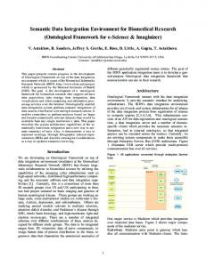
Biomedical decision support is the discipline which attempts to provide solutions to the aforementioned challenges (see Figure 1.1). Biomedical decision support draws methods from mathematics, statistics and artificial intelligence to model biomedical data. The general aim is to support the clinician in making decisions related to the clinical management of diseases. Typically this is done by learning a model based

1.2 Biomedical decision support

3

Figure 1.1: The difference between traditional cancer management and (BIO)medical decision support. On the left are possible data sources that can be used by the clinician or the model to predict clinical outcomes such as diagnosis, prognosis or response to therapy. Data from two omics layers have been used as an example for biomedical decision support: microarray and proteomics.

on biomedical data of which the clinical outcome is known. Then, this model is used to predict clinical outcomes of blinded data to investigate whether the model generalizes to new data. Research in the development of models to predict the clinical outcome of diseases has a history of more than three decades [4,5] and has found many applications [3, 6, 7]. The need for biomedical decision support arises when complex patterns exist in the data relevant for outcome prediction that cannot be extracted manually. For example, in many cases a multivariate model, a model based on more than one variable, may outperform any univariate model. A formal analysis using multivariate models could result in more complex models. A few examples of often used multivariate biomedical decision support models are, logistic regression, support vector machines (SVM) [8] or Bayesian networks [9]. Each of these methods has their own assumptions. Logistic regression assumes linear relationships between the variables and the clinical outcome while SVM allow to model certain non-linear relationships. All methods however have in common that they provide a formalized way of analyzing biomedical data instead of interpretation of clinical parameters based on a clinician’s expert knowledge. One decade ago, this field was focused mainly on medical decision support as most data were of a medical origin. Medical or clinical data consist of patient history, laboratory analysis, ultrasound parameters etc., depending on which data are relevant for the disease under study. Medical decision support modeling aims at using these data to improve prediction of clinical outcome compared to routine clinical management [3, 6, 7]. In 2001 however the first draft of the Human Genome project unlocked a vast resource

4

Introduction

of data which was previously unavailable [10]. For the first time it was possible to have an idea of all genes in the human genome. This accelerated research on a genomescale level and, combined with technological advances, led to the creation of large volumes of data. This has had significant consequences for diseases such as cancer. Additionally, this breakthrough makes decision support inevitable for biomedical data because of the size of genome-scale data which can range from 25,000 to a few 100,000 data points per patient. In this thesis we report the first attempt to develop methods for biomedical decision support that are able to cope with high dimensional and heterogeneous data sources. Furthermore, due to technological developments leading to a second generation of sequencing technologies (i.e. Solexa [11], SOLiD [12] and HeliScope [13]), soon the complete genome of an individual patient, a sequence of 3 billion letters per patient, will become available increasing both the opportunities and challenges in discovering patterns in biomedical data [14]. Recently additional genomes were sequenced among which the genomes of J. Craig Venter [15] and James Watson [16]. To illustrate that this evolution is nearby, the first steps to accomplish personalized genome sequencing have already been taken. The Welcome Trust Sanger institute together with the Beijing Genomics Institute and the National Genome Research Institute have embarked on a project that aims to sequence the genome of 1000 individuals across the world (www.1000genomes.org) which, when successful, will uncover natural variation in the human genome and may lead to more routine sequencing applications. The amount of data that became available due to technological breakthroughs and the amount of data that will become available in the near future, makes the development of biomedical decision support models a necessity.

1.3

The omics revolution: technological breakthroughs

The technological advances that lead to a flood of genome-scale data allow to characterize the different layers of organization in molecular biology. In this thesis these layers will be called ‘omics’ [17–19]. Figure 1.2 shows four omics and hypothetical relationships between the entities that define each omics layer: genes in the genome, mRNA in the transcriptome, proteins in the proteome and metabolites in the metabolome. This figure gives a hypothetical example of the connections in omics layers because currently not much is known on how these entities connect to each other on a genome scale level. In addition, this illustration is a simplified version of actual molecular biology since many other omics layers and entities exist (e.g. the epigenome and microRNA to name a few popular emerging layers). In this chapter, however we will focus on these four omics and describe how they can be measured. The first omics layer that was unlocked was the transcriptome using microarray technology. Microarray technology has its origin in the nineties [20, 21] and this technology allows to measure the expression of thousands of genes at once; possibly representing the whole genome. Usually a microarray consists of a selection of probes which are applied onto a solid surface and represent a number of genes. Next, reverse transcribed mRNA extracted from a sample such as a tumor can be hybridized with the probes on this surface resulting in expression levels of thousands of genes

1.3 The omics revolution: technological breakthroughs

5

Figure 1.2: Hypothetical example of interactions between genes, mRNA, protein and metabolites. If only the transcriptome is studied, only indirect interactions between genes can be modeled.

for every tumor sample that is hybridized (see Figure 1.3). Although the basis of microarray technology was established already before the completion of the human genome sequence, the knowledge of the human genome sequence allowed to design probes for both known and unknown genes. This greatly accelerated the application of microarray technology to genetic diseases such as cancer [22–24]. Secondly, the proteome has received increased attention due to the progress in mass spectrometry-based proteomics. The first study applying Surface Enhanced Laser Desorption Ionization (SELDI) technology on ovarian cancer samples [26], was heavily criticized [27–34]. Many others have used the same or similar technologies, such as Matrix Assisted Laser Desorption Ionization (MALDI), to profile diseases at the proteomic level [35–40]. In general, mass spectrometric measurements are carried out in the gas phase on an ionized sample. By definition, a mass spectrometer consists of an ion source, a mass analyzer that measures the mass-to-charge ratio (m/z) of the ionized sample molecules, and a detector that registers the number of ions at each m/z value [41]. Each step has a number of different technologies implementing these steps, therefore a large range of mass spectrometry methods can be developed each with their own properties and resolution (see Figure 1.4 for an introduction). In this way mass spectrometry-based proteomics allows to quantify and possibly identify a large number of proteins and peptides in one run. Thirdly, concurrently with microarray technology, the same principle was used to measure the copy number variations that are present in the human genome. This is done by measuring the DNA level or genome instead of the transcriptome. This technology was called array Comparative Genomic Hybridization (arrayCGH) and first applied on breast cancer already in 1998 [42–44] (See Figure 1.5). It only recently became clear that the copy number of genes can differ greatly between individuals [45–49]. A Copy Number Variation (CNV) is a region in the genome of 1kb or larger that has more or less copies compared to the reference human genome sequence. In Chapter 5 we will present our results on genomic data and show the importance of CNV for studying clinical outcome. These technologies have one concept in common namely a top-down approach instead

6

Introduction

Figure 1.3: Microarray technology. Panel A, two-channel microarray technology. First, mRNA from a patient and mRNA from a control sample are labeled with different fluorescent dyes. Then both patient and control sample are mixed and hybridized on a microarray containing probes representative of genes. After scanning the fluorescent intensities of each spot, relative expression levels are obtained for each gene represented on the array. Panel B, one-channel microarray technology. A sample is first labeled and applied separately onto a microarray. Hybridization is measured based on perfect match probes while background hybridization is measured using mismatch probes. The result is an absolute expression for each gene represented on the array. Adapted from Quackenbush [25]

of a bottom-up. Whether it is the genome, transcriptome or proteome, each technology attempts to capture these omics as a whole. This makes it possible to measure the transcriptomic, proteomic and genomic make-up of a tumor. These technologies provide also a holistic view of how the copy number of genes, their expression or the amount of protein changes instead of focussing on a single gene, mRNA or protein. In this thesis however we investigate if it is necessary to broaden the holistic view not only by looking at all entities within an omics layer but at the same time by integrating multiple omics layers. This field of research is often referred to as systems biology [17–19, 50].

1.4 The molecular biology of cancer

7

Figure 1.4: The basic proteomics setup is shown at the top left and consists of an ion source, a mass analyzer and a detector. a-f represent different configurations for Electrospray Ionization (ESI) and matrix-assisted laser desorption/ionization (MALDI). Taken from Aebersold and Mann [41].

1.4

The molecular biology of cancer

We have just introduced the large layers of molecular biology by focusing on the technologies that can unlock their respective omics. Here, we will focus in more detail on the entities that make-up each omics level by introducing the basics of molecular biology. In this thesis we exclusively study biomedical decision support related to cancer. Therefore, we will introduce molecular biology by describing the central dogma of molecular biology in the context of cancer and point out what can go wrong in cancer cells. The central dogma of molecular biology dictates that genes which are encoded in DNA form proteins through an intermediate called messenger RNA (mRNA). This is done in two steps: transcription and translation. The process of transcription is initiated by the binding of transcription factors together with RNA polymerase to form an mRNA molecule which is a perfect copy of the DNA template of a gene. Next, this mRNA is processed and transported out of the nucleus to the cytoplasm where it is translated into a protein by the ribosome complex. The general idea behind this dogma is that information flows from DNA over mRNA to the final protein product. However, more and more exceptions that contradict this idea have been found and the actual processes at the molecular level are more complex. First, the genome which contains the blueprints for genes and other functional elements is more variable than previously thought. A recent study showed that CNVs, whereby an individual has more or less copies of a gene compared to the reference genome, occur more than expected and overlap significantly with locations of disease related genes [45]. Moreover, the average size of these CNV is about 250kb which is more than the average size of a gene (approximately 60kb). This means that CNVs often

8

Introduction

Figure 1.5: Array comparative genomic hybridization (arrayCGH). First a test and reference sample are labeled with different fluorescent dyes. Next, they are applied onto a microarray containing genomic probes. The fluorescent intensities of each spot on the array represent the copy number of each probe. At the bottom, the log2 ratio is shown of all probes on chromosome 9. The probes indicated with the arrow on the left have a log2 ratio of -1 indicating loss of one copy whereas the probes indicated with the middle arrow have a normal log2 ratio.

contain genes and therefore their transcription will be affected. A second form of genomic variation, single nucleotide polymorphisms (SNP), defined as a one base difference in the DNA of two individuals, may determine differences in protein function or expression levels between individuals [51, 52]. SNPs can be implicated in cancer, possibly through interactions with environmental exposures, causing differences in prognosis or response to therapy between individuals. Another example of increasing complexity arises when considering alternative splicing of mRNA. Alternative splicing takes place after transcription and is a process whereby an mRNA molecule is spliced differently such that one gene can produce multiple forms or variants of the corresponding protein. This process is regulated by a group of proteins and small RNA molecules (i.e. the spliceosome). Other proteins can influence this process positively or negatively. Moreover, alternative splicing occurs in 40% to 60% of human genes [53]. There are already examples where this process is disturbed and gives rise to cancer [54] but in general it is thought that this occurs more often than observed now [55, 56]. Next, mRNA molecules are translated by the ribosome complex to become proteins. Proteins however can be post-translationally modified by adding a chemical group,

1.4 The molecular biology of cancer

9

for example a phosphate group. This process, called phosphorylation, changes the structure of the protein and thus affects its function. Other forms of post-translational modifications exist e.g. acetylation or glycosylation. The previously adopted paradigm ’one gene - one protein’ thus is violated. When taking into account alternative splicing and post-translational modifications, one gene can produce a variety of proteins. Potentially, each of the above introduced processes may be involved in the transformation of a healthy cell into a cancer cell. A cancer cell originates by evading the six hallmarks of cancer through one or more of these processes (see Figure 1.6) [57]. Eventually this results in fast, uncontrolled and abnormal cellular growth attacking healthy tissue. However, it is still unclear how these processes at different omics layers interact as a whole. Moreover, it is currently unknown which omics layer provides the most information to predict cancer outcome or whether integrating data from multiple omics improves predictive performance. The choice of omics to study a certain outcome of a specific disease is heavily biased towards literature or practical availability of methods. In this thesis, we hypothesize that combining information from different omics, can contribute to improve the characterization of a tumor and offer complementary information on the biological mechanisms in cancer cells. More specifically, we will attempt to accomplish this using Bayesian modeling.

Figure 1.6: The six hallmarks of cancer, taken from Hanahan and Weinberg [57].

10

1.5

Introduction

Bayesian networks and Bayesian modeling

So far we have focused on the data and on technologies to gather data for biomedical decision support. But what type of modeling did we use? Throughout this thesis we will focus on the use of Bayesian networks to model biomedical data. A Bayesian network is a probabilistic model that consists of two parts: a graph, encoding the dependencies between the variables and local probability models, specifying these dependencies [58]. Bayesian networks are considered a perfect combination of probability theory and graph theory [9, 59–63] and were put at the center of machine learning research by pioneering work of Judea Pearl in 1988 [58]. A Bayesian network is in essence a sparse representation of the full multivariate probability distribution which is in the case of biomedical data very large. For example, a microarray data set contains easily more than 20,000 mRNA expression levels which will result in a probability distribution of the same size. The sparseness of a Bayesian network is thus a very desirable quality for modeling biomedical data. Bayesian networks are a popular research topic and much research has been done on different aspects of Bayesian network modeling such as structure learning algorithms [58, 64, 65]. In biomedical research an important contribution was made by Friedman et al. [62]. They published the first application of Bayesian network modeling on microarray data. Secondly, an extension of Bayesian networks to the database world, called Probabilistic Relational Models (PRM), has been proposed and applied to microarray data [66]. In this thesis, we use the original Bayesian network definition and we extend existing Bayesian network learning algorithms to be able to integrate multiple heterogeneous and high-dimensional omics data. Despite its name, Bayesian networks can be learned in two ways: the Bayesian way or the non-Bayesian way. In this thesis, we preferred the paradigm of Bayesian modeling. Bayesian modeling centers around the concept of combining data with a person’s subjective belief to get an updated model which offers a compromise between the data and the subjective prior. The larger the data set, the lower the influence of the prior. Often it is difficult to specify a prior for a specific problem due to lack of any prior information. This can in most cases be solved by defining an uninformative prior reflecting the fact that nothing is known a priori. This is often seen as a disadvantage of Bayesian models. Our choice for Bayesian networks and the Bayesian paradigm for modeling data is motivated by the flexibility of Bayesian networks to model any kind of data and by the robustness against noise of probabilistic models in general. Bayesian networks can be tuned to each omics layer by defining dedicated probability distributions. Moreover, many omics technologies are noisy, e.g. microarray technology is notorious for its low signal-to-noise ratio. Probabilistic methods capture the noise naturally in the model which is not the case for deterministic methods. Additionally, the ability to define a subjective prior is considered an advantage in our setting. When modeling biomedical data many sources of information exist that can be used as a prior. For each omics layer some relationships may already be known, for example a protein-protein interaction indicating that two proteins bind or, a transcription factor and its targets indicating which genes it regulates. These data which are entity specific and which will be defined as secondary data sets in the next section

1.6 Objectives

11

allow defining a prior distribution on relationships between entities within and between omics. It is important to stress that in this thesis only the Bayesian network structure and its parameters are defined in a Bayesian way. This implies that no hyper-priors are used, which is typical in hierarchical Bayesian modeling [67]. In Chapter 2 we will discuss in more detail Bayesian modeling and how it compares to non-Bayesian modeling. The research on the use of Bayesian networks for modeling biomedical data has already a long standing tradition in SISTA. Previously, Antal et al. developed methods to integrate expert knowledge in the structure prior and the parameter prior of a Bayesian network model [68]. There results showed that when few data was available an expert prior on the possible structures of Bayesian networks improved the predictive performance. Secondly, a method was developed by Geert Fannes that captures expert knowledge in the form of a Bayesian network. Next, this knowledge is transformed in the form of virtual data sets as a prior for a neural network model [69]. In both projects the developed models were used to distinguish benign and malignant ovarian masses. Our research builds further on this experience and extends Bayesian network modeling and the use of structure priors to multi omics data.

1.6

Objectives

We have now introduced the technology, the data, our hypothesis and the model which allows us to define our goal. The main goal of this thesis is to develop a Bayesian network model able to integrate heterogeneous and high-dimensional data for biomedical decision support. We consider two specific types of data in our models: patient specific data or entity specific data (see Figure 1.7). We define patient specific data as a primary data source because it is the patient that is actually modeled and for whom we want to predict disease outcome. This means that clinical data and the previously introduced omics data are patient specific and thus primary data sources. Entity specific or secondary data sources are ‘orthogonal’ to primary data sources because they contain information on each entity within an omics layer. An entity depends on each omics layer for genomics the entities are genes, for transcriptomics mRNA, for proteomics proteins and for metabolomics metabolites. The integration of secondary data sources in Bayesian network models is possible because the relations between entities in an omics layer are explicitly modeled in a Bayesian network which is not the case when using for example an SVM with a linear or RBF kernel. [8]. We want to stress that in our setting the patient is modeled in a classification setting. This makes our definition of secondary data sources relative towards patient data. Other research has focused on classifying genes and frameworks have been developed that integrate many gene-related data sources (e.g. Lanckriet et al. [70]). In these genefocused frameworks our previously defined secondary data sources are at the center of attention and genes are classified into functional groups instead of patients. Thus, our definition of primary and secondary data only applies to patient-focused modeling. The use of secondary data sources is motivated by the fact that they are in most cases publicly available. Moreover, the number of databases containing potential secondary data sets has increased significantly [71]. Examples of such databases where secondary

12

Introduction

Figure 1.7: Visualization of the two specific types of data that are considered in this thesis. Primary or patient specific data such as clinical data, transcriptomic data, proteomic data and so on. Secondary data sources are ‘orthogonal’ to the primary data. In this figure possible secondary data sources are shown for the transcriptomic layer. data sources can be mined are BIOCARTA, KEGG [72] and Reactome [73]. Even the literature itself, in the form of published abstracts can be mined. Also for clinical data, in many cases, secondary data is available at relatively low cost in the form of expert knowledge. In most cases clinical data is low-dimensional making it possible for an expert in the field to deliver information that can be used as a secondary data source. Now we can define three important goals of this thesis: • Modeling primary data sources: Due to the heterogeneous nature of primary data sources, a different approach is needed for each primary data source. For example a clinical data set has well defined variables and is low dimensional. An arrayCGH data set on the other hand, consists of measurements for genomic clones which have to be transformed to CNVs. The latter is harder since the variables are not defined yet. We will demonstrate methods to model these two data sources and illustrate the flexibility of Bayesian networks. • Integrate primary data sources: We will develop algorithms to integrate primary data sources with Bayesian networks. Recently, model fusion became a hot topic in bioinformatics. However, no adequate models and methods have been developed and prior to our work little research has been done investigating data fusion for biomedical decision support. • Integrate secondary data sources: We will investigate the use of secondary data sources to facilitate the first two objectives. To the best of our knowledge,

1.7 Chapter-by-chapter overview

13

the use of secondary data to improve the performance of biomedical decision support models has not been investigated before.

1.7

Chapter-by-chapter overview

Figure 1.8 shows an overview how the different chapters are related to each other. Hereafter, we will give a brief description of each chapter.

Figure 1.8: Overview of the relationships between the different chapters of this thesis. • Chapter 2: This chapter gives an introduction on Bayesian methods in general and Bayesian networks specifically. We will focus on algorithms to learn Bayesian networks. Additionally, since throughout this thesis we will use discrete valued Bayesian networks, we will discuss this choice and introduce discretization algorithms. • Chapter 3: This chapter explains the background, aims and the data of the cancer sites that will be used in this thesis due to the availability of unique data gathered at the University Hospitals Leuven: ovarian cancer and rectal cancer. Additionally, the publicly available data sets used in this thesis are described. • Chapter 4: This chapter defines clinical data and discuss its use. We will focus on Bayesian network modeling of clinical data from the ovarian cancer case. • Chapter 5: In this chapter we describe genomic date. More specifically we will introduce copy number data and how it is modeled with a special class of Bayesian networks.

14

Introduction • Chapter 6: In this chapter we discuss methods for integrating primary data sources and illustrate them using publicly available data and data from the rectal cancer case. • Chapter 7: In the last chapter, we investigate the use of secondary data sources as priors in Bayesian network models. More specifically we describe our efforts when using literature abstracts as a prior for learning Bayesian network models of microarray data.

1.8

Specific contributions of this thesis

In this section, we highlight consecutively our specific contributions to this thesis with references to their publications. • Primary data integration: A Bayesian network integration method was developed to integrate clinical and microarray data. More specifically, we have developed and evaluated three methods to integrate clinical and microarray data from breast cancer patients using Bayesian networks: full integration, partial integration and decision integration. The difference in these integration methods is when integration takes place during model building: early, intermediate or late. We have applied these methods for the prediction of the prognosis of breast cancer patients. Our results show that the partial integration method had the best performance. The final model contained three clinical variables and 13 genes that were needed for the prediction of prognosis of breast cancer patients. This work was presented at the 14th Annual international conference on Intelligent Systems for Molecular Biology and published in Bioinformatics (Gevaert et al. 2006). An extension of this framework was developed to integrate microarray and proteomics data and is currently under review (Gevaert et al. submitted). This work is described in Chapter 6. • Secondary data integration: The Bayesian network framework was extended to include secondary data sources as structure priors. Due to the high dimensionality of omics data, expert priors are not feasible therefore we investigated the use of automatically generated priors to restrict the model space. More specifically, we studied whether the use of priors based on text mining of literature abstracts improved predictive performance of the models. Prior to this work, there were no previous reports on the use of text priors in a classification setting. We applied our methods and four data sets and the results showed that in each case using the text prior improved the prediction of prognosis of cancer patients. This work was presented at the pacific symposium on biocomputing (Gevaert et al. 2008) and a general framework was published in an issue on reverse engineering biological networks by the Annals of the New York Academy of Sciences (Gevaert et al. 2008). These results are described in Chapter 7. • Modeling clinical data: We applied Bayesian network modeling to predict malignancy in ovarian masses based on clinical data. This involved the prospective testing of a Bayesian network model. This work was presented at

1.9 Other research

15

the 18th World Congress on Ultrasound in Obstetrics and Gynecology and a full paper is submitted to Ultrasound in obstetrics and gynecology (Gevaert et al. 2008). The results are described in Chapter 4. • Modeling arrayCGH data: A special class of Bayesian networks called hidden Markov modeling, was used to differentiate BRCA-mutated and sporadic ovarian cancers. We specifically investigated the molecular mechanisms that cause carcinogenesis in BRCA mutated tumors. This work will be presented at the 12th biennial meeting of the international gynecologic cancer society (Leunen et al. 2008). The results are described in Chapter 5.

1.9

Other research

Due to the interdisciplinary nature of the research an extensive collaboration with clinicians of the University Hospitals Leuven arose. This produced a number of research projects which are not explicitly included in this thesis. We have contributed to the research on pregnancies of unknown location (PUL) in a collaboration with Prof. Dirk Timmerman and with Prof. Tom Bourne, Dr. Emma Kirk and Prof. George Condous at St Georges Hospital in London (now at University of Sydney). This involved investigating the use of expert priors in combination with Bayesian network models to predict ectopic pregnancies in the PUL population. The results were published in Human Reproduction (Gevaert et al. 2006). Secondly, in collaboration with Prof. Ignace Vergote and Prof. Dirk Timmerman we evaluated a model built on a pilot microarray data set of ovarian cancer patients [74], on an independent data set. This model was a Least Squares Support Vector Machine (LSSVM) which belongs to the class of kernel methods. The LS-SVM model was used to predict therapy response in ovarian cancer patients. The results were recently published in BMC Cancer (Gevaert et al. 2007). More recently, we are also investigating the use of mass spectrometry data, including both Surface enhanced laser desorption ionization time-of-flight (SELDI-TOF) and Matrix assisted laser desorption ionization time-offlight (MALDI-TOF) approaches, to predict therapy response in ovarian cancer and other gynecological tumors. Additionally, in cooperation with Dr. Ann Smeets we are investigating the use of microarray data and least squares support vector machines to predict lymph node invasion in breast cancer patients. We also cooperated in the research to investigate mathematical decision trees versus clinician based algorithms in the diagnosis of endometrial disease in cooperation with Prof. Dirk Timmerman and Dr. Thierry Van den Bosch. The results were published as an abstract (Van den Bosch et al. 2007) and a full paper (Van den Bosch et al. 2008) in Ultrasound in Obstetrics and Gynecology. Next, in cooperation with Prof. Thomas D’Hooghe we investigated the use of mathematical models to predict the presence of endometriosis. This ongoing research includes the use of ELISA, tissue proteomics (SELDI-TOF), serum proteomics (SELDI-TOF) and nerve fiber density as a data source and has been presented at two international meetings (Kyama et al. 2007, Kyama et al. 2008). Currently, three full

16

Introduction

papers of which we are a co-author are submitted (Mihalyi et al., Kyama et al., Bokor et al.). Next, an ongoing cooperation with the Bioinformatics and Neurology group from the Erasmus MC University Medical Center Rotterdam centers on the investigation of glioma development. To accomplish this we are using unsupervised and supervised analysis to define molecular subgroups and develop models to aid diagnosis and treatment. In cooperation with Prof. Jos van Pelt, Prof. Chris Verslype and Dr. Louis Libbrecht (now at University Hospitals Ghent) of the hepatology section we aided in the development of models to predict prognosis in hepatocelullar carcinoma. Finally, in cooperation with Anneleen Daemen a kernel framework is being built to integrate omics and clinical data. This work has been presented at the Pacific Symposium on Biocomputing (Daemen et al. 2008). Additionally, the work focused on the analysis of arrayCGH data with kernel methods has been presented at the 12th International Conference on Knowledge-Based and Intelligent Information and Engineering Systems (Daemen et al. 2008). A follow-up paper will be presented at the Pacific symposium on biocomputing in 2008 (Daemen et al. 2009). Currently, a full paper on the kernel integration framework is submitted (Daemen et al.).

Chapter 2

A Bayesian network primer “Graphical models are a marriage between probability theory and graph theory. They provide a natural tool for dealing with two problems that occur throughout applied mathematics and engineering – uncertainty and complexity – and in particular they are playing an increasingly important role in the design and analysis of machine learning algorithms. Fundamental to the idea of a graphical model is the notion of modularity – a complex system is built by combining simpler parts. Probability theory provides the glue whereby the parts are combined, ensuring that the system as a whole is consistent, and providing ways to interface models to data.” – Michael Jordan 1998 –

There exist many types of models that can accomplish the goals of biomedical decision support. In this thesis we have chosen the class of Bayesian modeling and more specifically the Bayesian network model. In this chapter we will argue this choice, which as we will explain, are independent of each other. We will focus on algorithms to learn Bayesian networks, how to incorporate prior information in a Bayesian network model and we will describe in detail an inference algorithm. Finally, we will argue our choice for discrete models and discuss algorithms for discretization of continuous data.

2.1

Introduction

This quote from Michael Jordan emphasizes the potential of Bayesian network modeling and when interpreted through systems biology glasses many of the points raised make sense. Biomedical data is both characterized by uncertainty in the form of noise and by the complexity of how genes, through their transcripts, form proteins 17

18

A Bayesian network primer

steering metabolic processes that determine the fate of the cell. Furthermore the modularity of Bayesian networks is mirrored in modularity in biological networks [75–77]. Recent research results point to highly modular blocks that are connected by hubs. This is evidenced by the so-called party hubs observed in protein-protein interaction networks [78] or the cancer modules discovered by an extension of Bayesian network theory to the database world [66]. Before 1988 Bayesian networks received little attention. It was due to pioneering work of Judea Pearl in 1988 who developed an algorithm for inference that Bayesian networks became a viable research topic [58]. Inference is the prediction of unseen events based on observed evidence using a Bayesian network. Pearl called this algorithm “the message passing algorithm” and it formed the basis for later work on inference and made it for the first time possible to perform exact inference in Bayesian networks. This algorithm and its successors in combination with increasing computer power augmented the usefulness of Bayesian networks [60,79]. Now, the focus was on learning Bayesian networks and many algorithms, Bayesian and non-Bayesian, were developed and applied to many different applications [80, 81]. Despite their name Bayesian networks are essentially not Bayesian. Bayesian networks are called Bayesian because they use Bayes’ rule for inference, the prediction of unseen events when model building is already finished. The “Bayesian” in Bayesian networks thus does not refer to the manner that this model is built. Both Bayesian and non-Bayesian, also called frequentist, algorithms exist to learn the structure and parameters of a Bayesian network model [59]. To put this into perspective, we will first shortly discuss the Bayesian and the frequentist approach to general statistical inference followed by an introduction on Bayesian networks. We specifically focus on algorithms to learn Bayesian networks and our motivation of using discrete valued Bayesian networks, a subclass of Bayesian network models. Next, due to this choice for discrete valued Bayesian networks we describe methods to discretize data. Finally, we describe the Bayesian network software implementation that was used in this thesis.

Figure 2.1: The frequentist paradigm: parameters are unknown and are estimated using the data. The uncertainty in the parameters is estimated by considering parallel universes that created slightly different data sets which can be used to repeat the parameter estimation. These parameters estimates capture the uncertainty of the actual parameter estimate.

2.2 Two paradigms for statistical inference

2.2

19

Two paradigms for statistical inference

The frequentist paradigm is based on the view that data is generated by a process with unknown but fixed parameter θ [63]. Based on data θ is estimated by choosing this parameter such that the likelihood of observing the data is maximal (see Figure 2.1). In most cases this corresponds to the popular maximum likelihood estimate however other methods exist. Uncertainty in this estimate is captured by repeating the data generating process which results in a probability distribution over θ representing the uncertainty. Obviously, in many cases the data generating process cannot be repeated such that this exercise is a hypothetical one and is accomplished using techniques such as bootstrapping [82]. The Bayesian formalism does not regard the parameters, θ, to be fixed but rather

Figure 2.2: The Bayesian paradigm: parameters are considered to be randomly distributed and are modeled using a probability density function which is estimated based on the data. defines it as a random variable [63]. Intuitively a random variable is a mapping from the sample space to real numbers. Then, θ is considered to be distributed according to some probability density function specifying the probability of each possible outcome in the sample space. To overcome the difficulty of attaching a probability to a nonrepeatable event, subjective uncertainty is introduced (see Figure 2.2). The uncertainty of θ is captured by the well known Bayes’ rule. The subjective prior is multiplied with the likelihood to form the posterior distribution: p(θ|D) ∝ p(D|θ)p(θ)

(2.1)

This implies that inference is done only on the data gathered instead of the cumbersome parallel universes in the frequentist approach. Figure 2.3 shows an example of the application of Bayes rule and the influence of the prior. In this example we assume a binary event and its true probability of occurring is 0.5, for example flipping a coin. Three situations are depicted: a weak prior, a strong prior and an uninformative prior. In each situation the data is the same: there are 25 observations of heads and 25 observations of tails. Figure 2.3 shows that in the case of the weak prior, the posterior is less peaked compared to the strong prior. The uninformative prior on the other hand has little influence and only the data determine the posterior. Throughout this text we have favored a Bayesian approach in most cases motivated from a practical point of view. In many situations where no information a priori is

20


Figure 2.3: Bayes rule in practice. The prior, likelihood and posterior are shown for a binary event, for example flipping a coin. The probability θ of either outcome is 0.5 and the data consists of 25 observations of each outcome. The first row shows the influence of a weak prior, the second row of a strong prior and the last row of a uniform prior.

available, it is difficult to determine a suitable prior. In these cases uninformative priors are used which are not always straightforward [67]. However, in our case prior information is often available thus increasing the usefulness of the Bayesian approach over the frequentist approach. First we will define Bayesian networks and its concepts followed by a description of learning algorithms. Next, we will define priors for Bayesian networks and how inference is done. Finally, we describe discretization algorithms.

2.3 2.3.1

Bayesian networks Definition

A Bayesian network is a probabilistic model that consists of two parts: a dependency structure and local probability models [9, 58]. Figure 2.4 shows an example of a Bayesian network related to lung cancer. The dependency structure specifies how the variables are related to each other by drawing directed edges between the variables without creating directed cycles. Each variable depends on a possibly empty set of other variables which are called the parents: p(x1 , ..., xn ) =

n Y i=1

p(xi |P a(xi ))

(2.2)

2.3 Bayesian networks

21

Figure 2.4: A toy example of a Bayesian network with four binary variables. The conditional probabilities are shown next to each node. The probabilities are chosen realistically.

where P a(xi ) are the parents of xi . Usually the number of parents for each variable is small therefore a Bayesian network is a sparse way of writing down a joint probability distribution. This is an important advantage of Bayesian networks because this allows a dramatic decrease in the number of parameters that is needed to specify a probabilistic distribution over a number of variables. In the discrete case, the full joint probability distribution for n binary variables needs 2n − 1 probabilities or parameters that have to be specified; one probability for each instantiation of the variables. For example, the Bayesian network in Figure 2.4 needs 11 parameters vs. 31 parameters that are needed for the full joint distribution. The second part of this model, the conditional probability distributions, specifies how the variables depend on their parents. Throughout this thesis we systematically used discrete-valued Bayesian networks therefore these conditional probability distributions can be represented with Conditional Probability Tables (CPTs). Such a table specifies the probability that a variable takes a certain value given the value of its parents. In Figure 2.4 the CPTs for each variable are shown alongside each node.

2.3.1.1

Markov blanket

An important concept of Bayesian networks is the Markov blanket of a variable. The Markov blanket of a variable is the set of variables that completely shields of this variable from the other variables. This set consists of the variable’s parents, children and its children’s other parents (see Figure 2.5). A variable in a Bayesian network is conditionally independent of the other variables given its Markov blanket. Conditional independency means that when the Markov blanket of a certain variable x is known, adding knowledge of other variables leaves the probability of x unchanged [83]. This is

22


an important concept because the Markov blanket is the only knowledge that is needed to predict the behavior of that variable. For classification purposes we use the concept of the Markov blanket to identify the minimal set of variables that are needed to predict the clinical outcome.

2.3.2

Bayesian network learning

A Bayesian network is thus composed of two parts: a structure and its conditional probability distributions. Depending on the data a Bayesian network is manually created or learned from data. In practice manual specification of the structure and/or the conditional probability distributions of a Bayesian network is only possible when the number of variables is limited. For example when modeling clinical data the dimensionality is limited to a few dozen variables and it is feasible to specify a Bayesian network by hand based on expert knowledge. In all other cases, when modeling genome-scale data, the number of variables ranges from a few hundred to more than thousand variables, which prohibits manual specification of a Bayesian network. In these cases, algorithms are used to learn a Bayesian network from data. Due to the duality of Bayesian networks, two steps have to be performed during the learning process: structure learning and parameter learning. Structure learning corresponds to learning the arrows of Figure 2.4 or the identity of the the parents P axi of variable xi in equation 2.2. Parameter learning corresponds to learning the probabilities in the CPTs of Figure 2.4. When finished, a Bayesian network can be used to predict unseen data. Subsequently, we describe in more detail how the structure and parameters are estimated. 2.3.2.1

Structure learning

First, the structure is learned using a search strategy. Since the number of possible structures increases super-exponentially with the number of variables, the well-known greedy search algorithm K2 [84] was used in combination with the Bayesian Dirichlet (BD) scoring metric [80]: # " qi ri n Y 0 0 Y Y Γ(Nijk + Nijk ) Γ(Nij ) , (2.3) p(S|D) ∝ p(S) 0 +N ) 0 ) Γ(Nij Γ(Nijk ij i=1 j=1 k=1

with Nijk the number of cases in the data set D having variable i in state k associated with the j-th instantiation of its parents in current structure S. Data set D contains n variables which are fixed and known before Bayesian network learning Pri starts. Next, 0 Nij is calculated by summing over all states of a variable: Nij = k=1 Nijk . Nijk 0 and Nij have similar meanings but refer to prior knowledge for the parameters. When 0 no knowledge is available they are estimated using Nijk = N/(ri qi ) [59] with N the equivalent sample size, ri the number of states of variable i and qi the number of instantiations of the parents of variable i. Γ(.) corresponds to the gamma distribution. Finally p(S) is the prior probability of the structure which we will define later in this chapter.


23

Figure 2.5: The Markov blanket of variable A is composed of the variable’s parents, its children and its children’s other parents. The Markov blanket variables are encircled. Using Equation 2.3 we can now score structures using the K2 search strategy. K2 consists of a greedy search combined with a prior ordering of the variables. This ordering restricts the search space by only allowing parents if they precede the current variable in the ordering. Then K2 iteratively tries to find the best parents for each variable separately by starting with an empty set of parents and incrementally adding the best parents. When the addition of a parent does not increase the score, the algorithm stops and moves on to the next variable in the ordering. Since the ordering of the variables is not known in advance, the model building process is iterated a number of times with different permutations of the ordering. Then, the network with the highest score is chosen. Randomly permuting the ordering of the variables is similar to randomly changing a number of edges in the network and restarting the search strategy. Both methods are used to escape local minima in the search space.

2.3.2.2

Parameter learning

The second step of the model building process consists of estimating the parameters of the local probability models corresponding with the dependency structure. Since we only use discrete variables in our Bayesian network models, we will discuss how the parameters in a CPT are learned. For each variable a CPT exists that consists of a set of parameters. Each set of parameters is given a uniform Dirichlet prior: 0 0 0 p(θij |S) = Dir(θij |Nij1 , ..., Nijk , ..., Nijr , S) i

(2.4)

with θij a parameter set where i refers to the variable and j to the j-th instantiation of the parents in the current structure. θij contains a probability for every value of the variable xi given the current instantiation of the parents. Dir corresponds to 0 0 the Dirichlet distribution with (Nij1 , ..., Nijr ) as parameters. In this thesis no prior i 0 information will be integrated in the parameter prior therefore the Nij1 parameters of the Dirichlet distribution are chosen un-informatively [59]. Parameter learning then consists of updating these Dirichlet priors with data. This is straightforward because the multinomial distribution that is used to model the data, and the Dirichlet distribution

24


that models the prior, are conjugate distributions. This results in a Dirichlet posterior over the parameter set: 0 0 0 p(θij |D, S) = Dir(θij |Nij1 + Nij1 , ..., Nijk + Nijk , ..., Nijr + Nijri , S) i

(2.5)

with Nijk defined as before. We summarized this posterior by taking the Maximum A Posteriori (MAP) parameterization of the Dirichlet distribution and used these values to fill in the corresponding CPTs for every variable. Using MCMC could improve our current set-up because this technique allows devising the complete posterior distribution however at a higher computational cost [85].

2.3.3

Priors

We specifically chose the Bayesian framework because of the flexibility of incorporating information in the learning process through priors. We already stated in the introduction that many secondary or entity specific data sources exist that can be incorporated in priors. A number of examples of possible sources of prior information are known interactions between proteins (BIND, IntAct, HPRD, ...), metabolic and signaling pathways (BIOCARTA, KEGG [72], Reactome [73]) and the literature. For clinical data prior information is also available in the form of expert knowledge. The duality of Bayesian networks is also translated in its ability to incorporate prior information. Prior information can be incorporated in both steps of the learning process in the form of a structure prior and a parameter prior. It is important to stress that in this thesis only the Bayesian network structure and its parameters are defined in a Bayesian way. This implies that no hyper-priors are used, which is typical in hierarchical Bayesian modeling [67]. 2.3.3.1

Structure prior

Previously two approaches have been used to define informative prior distributions over Bayesian network structures [68]. First, there are penalization methods that start from a prior structure and score structures based on the difference with the prior structure [59]. Secondly, there are pairwise methods which define the prior probability of a Bayesian network structure by combining individual edge scores between variables. This method assumes that being a parent of some node is independent of any other parental relation. In this thesis the second approach was chosen because our secondary data sources are in most cases in the form of pairwise relationships. Moreover this type of structure prior is decomposable which has important computational advantages. The structure prior decomposes as: p(S) =

n Y

p(P a(xi ) → (xi ))

(2.6)

i=1

with P a the parents of xi . Each parent set can be learned independently of other parental relationships which preserves the decomposability of the Bayesian Dirichlet score. We can thus replace the P (S) in equation 2.3 and bring the structure prior within


25

the outer product: p(S|D) ∝

n Y

p(P a(xi ) → (xi ))

i=1

qi Y j=1

"

ri 0 0 Y Γ(Nijk + Nijk ) Γ(Nij ) 0 0 ) Γ(Nij + Nij ) Γ(Nijk

# (2.7)

k=1

In the current domain there are many variables therefore it is computationally less expensive to update the prior locally instead of globally for every move that is made in the search space. This would not be possible when using a penalization method to define the structure prior which would severely increase computational times. The probability of a local structure (i.e. p(P a(xi ) → xi )) is then calculated by multiplying the probability that there is an edge between the parents of xi and the probability there is no edge between the other variables and xi : Y Y p(P a(xi ) → xi ) = p(z → xi ) p(y 9 xi ) (2.8) z∈P a( xi )

y ∈P / a( xi )

where 9 means no edge between y and xi . The p(z → xi ) and p(y 9 xi ) come from the prior data source and are defined depending on its nature. These individual edge probabilities can be represented in a matrix and are used to guide model search through their influence on Equation 2.3. Depending on the type of prior data, the structure prior can be sparse or non-sparse. In the latter case many edges have a strong prior which will result in very complex networks. A fully connected Bayesian network can explain any data set, therefore network complexity should be reduced. Rather than using the prior edge probabilities directly, we will introduce an extra parameter ν, called the mean density, which controls the density of the networks that will be generated from the distribution. We will transform all the matrix elements in the prior with an exponent ζ such that the average of the mean number of parents per local substructure is in agreement with the given mean density [68]. Finding the exponent ζ that gives rise to the correct mean number of parents can be done with any single variable optimization algorithm. This parameter allows to control the complexity of the networks that will be learned. 2.3.3.2

Parameter prior

We already mentioned that the best choice for a prior for the parameters in a CPT is the Dirichlet distribution. Equation 2.4, which we repeat here for convenience, illustrates the possibility for incorporating information at the second level of a Bayesian network. 0 0 0 p(θij |S) = Dir(θij |Nij1 , ..., Nijk , ..., Nijr , S) i

(2.9)

This Dirichlet distribution forms the prior for each parameter set θij . It is determined 0 0 by its parameters, called hyper-parameters, Nijk . The Nijk can be interpreted as the number of times variable i has been observed with value k and with the j − th parent instantiation. This type of knowledge is not easily available from the previously mentioned secondary data sources. Moreover, as the structure changes the parent set of each variable i can change requiring a different parameter prior. This could lay a large computational burden on learning algorithms instead of aiding in the learning

26


process. Expert knowledge on the other hand can be integrated in a parameter prior. When using the example of Figure 2.4, a parameter prior for variable xi , the history of lung cancer, could be the number of smokers in the general population based on a study from literature. A more complex example is variable x5 , mass seen on X-ray, which has one parent, the presence of lung cancer. For x5 the parameter prior could come from another study which has X-ray data of lung cancer patients by counting the number of patients with lung cancer that have or don’t have a mass on X-ray. However, suppose the structure changes and the link between x3 and x4 is removed, this would invalidate this parameter prior. This makes the use of a parameter prior a cumbersome task which can only be undertaken when the dimensionality of the data is limited, for example when modeling clinical data. We have investigated the use of expert information in the parameter prior of a Bayesian network by distinguishing ectopic pregnancies in a population of pregnancies of unknown location (PUL). There we showed that using a parameter prior based on expert knowledge improves classification performance. The results were published in Human Reproduction [7].

2.3.4

Inference

When model building is finished a Bayesian network can be used for prediction of an alternative hypothesis based on evidence. In the context of Bayesian networks this is called inference. We used the probability propagation in tree of cliques algorithm (PPTC) developed by Lauritzen and Spiegelhalter [65], refined by Jensen [64], to predict the state of the outcome variable (i.e. the diagnosis of ovarian masses). Here we will briefly describe the PPTC algorithm, for a more elaborate description we refer to an excellent review by Huang and Darwiche [86]. To illustrate the objective of the PPTC algorithm, we will give an example based on Figure 2.4. Using this algorithm one can compute the probability of lung cancer given that a mass is visualized on X-ray and the patient does not smoke: P (x3 |x1 = f alse, x5 = true). More generally PPTC allows to compute P ({xi }|{xj }) where {xi } is a collection of variables of which we want to compute its value and {xj } is a collection of other variables of which we have evidence. In short we ask what is the probability of xi given that we know xj . PPTC consists of two steps: construction of the clique tree and handling the evidence. A clique tree is in the literature also known as join tree, junction tree, tree of belief universes, cluster tree, among others. The clique tree is an undirected tree where each node represents a cluster of variables and each edge represents the intersection of the adjacent clusters. A Bayesian network is transformed in its corresponding clique tree by applying some graphical steps. The idea behind this step is to create a tree where nodes represent collections of variables from the original Bayesian network. This is necessary because the next step in the algorithm, handling the evidence requires a tree structure. After initialization of the clique tree, the evidence is entered and propagated until the tree is consistent. Once the tree is consistent our probability P (x3 |x1 = f alse, x5 = true) can be calculated.

2.4 Evaluation measures

2.4

27

Evaluation measures

When inference is viewed in the context of biomedical decision support, inference is done to predict the outcome variable P (outcome|data). To assess the performance of a model for predicting clinical outcomes we adopt the concepts of training and test set that form the basis of classification in machine learning. Typically a model is built only based on the training set. Next, the model is tested on a set of new patients called the test set which was not used for training the model. The performance of the model on this test set can be used to compare with other models in an unbiased way. Performance can be measured based on a number of different metrics. In this thesis we primarily used the ROC curve and the area under the ROC curve (AUC). In the next section we will explain this in detail.

2.4.1

Receiver Operating Characteristic curve

In most cases, we used Receiver Operating Characteristic curves (ROC) to evaluate the predictive performance of the developed models [87]. More specifically, the models were compared using the Area Under the ROC curve (AUC) which can be interpreted as the probability of being able to distinguish a sample with disease from a sample without the disease. To explain the meaning of a ROC curve first we have to explain sensitivity and specificity of a test. Figure 2.6 shows a typical situation of a two-class problem. In this situation one class is considered as the positive and the other class is considered to be the negative class. In the rows are the patients that are classified by the model in either of these two classes. In the columns is the true class of each patient. This gives four definitions: • true positive (TP): a positive patient classified as a positive • false positive (FP): a negative patient classified as a positive • false negative (FN): a positive patient classified as a negative • true negative (TN): a negative patient classified as a negative Based on these definitions we can define the following concepts: • sensitivity: TP/(TP+FN) • specificity: TN/(FP+TN) • positive predictive value (PPV): TP/(TP+FP) • negative predictive value (NPV): TN/(FN+TN) • accuracy: (TP+TN)/(TP+FP+FN+TN) Many models however do not just predict whether a patient is a positive or negative but output a continuous value e.g. the probability of being a positive. This means that we can generate many tables as in figure 2.6 depending on the threshold on the

28


Figure 2.6: Truth table: in the rows are the predictions by the model in two classes, positives and negatives. In the columns are the actual classes of the patients. This gives four situations: true positives, false positives, false negatives and true negatives which are used to define sensitivity, specificity, positive predictive value, negative predictive value and accuracy. See the main text for these definitions.

Figure 2.7: The Receiver Operating Characteristic curve or ROC curve. On the left a general ROC curve is depicted with one operating point highlighted. The ROC curve in the middle corresponds to a random model. The ROC curve on the right corresponds to a perfect model.

continuous probability. Now we can define a ROC curve which is the sensitivity vs. 1 minus the specificity for all possible thresholds. Each point of the ROC curve thus corresponds to a sensitivity and specificity of the test and is called an operating point. Figure 2.7 shows an example of a ROC curve. The advantage of the ROC curve is that it is independent of the threshold that is chosen. Choosing a threshold after all depends heavily on the disease, in some cases a high sensitivity is required while in other cases a high specificity is needed. The most important property of the ROC curve is the area under the ROC curve (AUC)

2.5 Discretization

29

which can be interpreted as the ability of the model to distinguish the two classes. More formally the AUC is the probability of being able to distinguish a positive and a negative from each other. An AUC of 50% corresponds to a random model the model is not able to discriminate the two classes better than flipping a coin. An AUC of 100% corresponds to a perfect model which always can discriminate the two classes independent of the operating point.

2.4.2

Cross validation and randomization

When the number of samples is limited however, the data set may be too small to have an independent test set. In this case the performance is estimated using cross-validation methods. Instead of using an independent test set cross validation splits the data up in a number of equal parts for example 10. Each part is called a fold and the number of folds depends on the data set size. In general this method is called k-fold cross validation depending on the number of folds. First a model is built on all folds except one and tested on the left-out fold. This is iterated for all folds such that each fold is used once as an independent test set. The performance of the model on each of the folds is then aggregated to have a final performance. The performance can be measured using the previously introduced evaluation metrics such as accuracy or AUC. Leave-one-out cross validation (LOO-CV) is an extreme form of k-fold cross validation where the number of folds is equal to the number of samples. LOO-CV is mostly used for very small data sets. A downside of cross validation is that the results heavily depend on how the data is split into folds. If by accident a subgroup of similar samples are put into the same fold, this fold may not be representative of the population. This can be remedied by using other methods such as randomization. Randomization randomly assigns patients to train or test set independently for each randomization.

2.5 2.5.1

Discretization Motivation

Throughout this text always discrete valued Bayesian networks were used. This means that continuously valued variables whether these are clinical or biological of origin are discretized into a finite number of bins. We have chosen discrete valued Bayesian networks inspired by the argumentation of Hartemink [88]. Firstly, the space of arbitrary continuous distributions is large and it is unclear which continuous distribution should be used to model the relationship between a parent and a child. A solution often advocated could be to restrict ourselves to the use of Gaussian Bayesian networks. This class of models however assumes linear interactions between the variables which is too simplistic when modeling biomedical data. Secondly, the discretization of gene expression values into a limited set of states seems a plausible abstraction. When studying cancer due to the experimental setup, gene products are assumed to be in steady state such that the expression of a gene is in for example one of three states: under-expression, off or over-expression. Additionally, discrete-valued

30


Bayesian networks allow to represent arbitrary discrete probability distributions with a limited number of parameters. Therefore, to avoid the enormous space of non-linear continuous distributions or too simplistic continuous distributions such as Gaussian conditional probability distributions, we chose the process of discretization where we specifically tried to minimize any loss of relationships between the variables.

2.5.2

Algorithms

2.5.2.1

Simple discretization algorithms

Two simple discretization methods are quantile discretization and interval discretization. In quantile discretization the observations of a variable are divided in bins by sorting the observations and putting an equal number of observations in each bin. For example of the data is discretized in four bins, the first quartile of the observations is put in the first bin, the second quartile in the second bin and so on. Interval discretization divides the range of the observations in equal parts. Interval discretization thus puts the observations in bins of equal size in the measurement scale of the observations instead of bins of equal number of observations. This simple discretization method is therefore sensitive to outliers since they can severely influence the location of the bins.

2.5.2.2

Information preserving discretization

The previous discretization methods are simple methods since they are operated in an univariate manner. Each gene is discretized independently of the other genes. However, this may cause that the relationships between the genes are lost. Figure 2.8 shows an example that illustrates this concept with two genes. Since we are attempting to learn the relationships between variables the loss of relationships between variables is critical. The essence of representing omics data with Bayesian networks is the relationships between the variables in the form of (in)dependence relationships. To remedy this we used an information preserving discretization method developed by Hartemink [88]. This algorithm discretizes a data set by starting from a large number of bins per variable and iteratively joining neighboring bins by minimizing the loss of mutual information. First, a simple discretization method for example quantile or interval discretization is used to discretize the variables in a large number of bins (e.g. 30). Then the algorithm starts by iterating over the variables and for each variable all possible combinations of neighboring bins are considered. The operation which results in the smallest loss of mutual information with respect to each of the other variables is chosen. This is done for every variable and until the variables all have the desired number of bins (e.g. 3). In this manner, the bins are chosen in a multi-variate manner taking into account the relationships between the variables. We slightly adapted this algorithm in the context of discrete clinical variables by also taking into account the mutual information with these clinical variables. The discretization was thus adapted such that the loss of relationships between all types of variables is minimized.

2.5 Discretization

31

Figure 2.8: Information preserving discretization: The top panel shows an example of discretizing two genes separately. The discretization on the right seems acceptable. When considering both genes together in the bottom panel the previous discretization is suboptimal. Much of the relationship between the two genes would get lost. When considering both variables together, the discretization is done differently.

The disadvantage of this information preserving discretization is that it is computationally more expensive compared to simple discretization methods. Especially when taking into account the relationships with the clinical variables and the clinical outcome. In this case the discretization is done supervised and thus information from the outcome variable is used to build the model. Therefore the discretization has to be done inside the previously introduced cross-validation methods.

2.5.3

Implementation

The software used in this thesis is based on a combination of C++, java, matlab and perl. The Bayesian network algorithms were previously implemented in C++ by Geert Fannes and Peter Antal. Functions to enable the integration of primary and secondary data sources were added to the core Bayesian network software already present. Matlab scripts based on the thesis of Hartemink [88] were used to implement the multivariate discretization. Next, Matlab scripts were used to construct the structure priors in combination with Java Lucene for indexing pubmed in cooperation with Steven Van Vooren. Finally, perl scripts were used to implement the different workflows for integrating primary and secondary data sources. A typical analysis of learning a Bayesian network took between 5 and 30 minutes depending on the data set size ranging from 10 to 200 variables. When multiple data sets are integrated the computational load should be multiplied with the number of data sources. Finally, this computational cost should be multiplied with the number of

32


cross-validation or randomizations that is performed. During our PhD research initially all analysis were done on a desktop computer followed by the use of a 12-node cluster of AMD dual core opteron 2.4 GHz servers with between 4 and 16 GB RAM memory. Finally, we used the high performance cluster of the KU Leuven containing 256 nodes to parallelize cross-validation runs.

2.6

Conclusions

In this chapter we have introduced the model that we will use primarily in this thesis: the Bayesian network. We described Bayesian methods in general and Bayesian networks in detail. As evaluation measures we introduced an important concept called the ROC curve and the AUC which will be used repeatedly throughout this thesis. Finally, we discussed and motivated discretization of the data. In the following chapter we will describe in detail the cancer sites where we investigated the use of biomedical decision support.

Chapter 3

Ovarian and rectal cancer: background, aims and data. “In current clinical practice, the majority of patients with early breast cancer receive some form of systemic adjuvant therapy, which may have important side effects and which puts considerable burden on health care costs. Although guidelines have been developed to assist clinicians in selecting patients who should receive adjuvant therapy, it still remains a challenge to distinguish those patients who would really need adjuvant systemic therapy from those who could be spared such treatment.” – Desmedt et al., Clinical Cancer Research, 13(11), 3207-3214, 2007 –

Each cancer site has its specific challenges or problems that have to be addressed. For example, ovarian cancer is often called the “silent killer” due to absence of symptoms in early stages. Clinicians also face challenges when deciding which therapy to use. For example, breast cancer patients are often overtreated while it is known that approximately 25% of node positive patients will remain free of disease even without adjuvant therapy. In this chapter we will describe the background of the cancer sites that are studied in these thesis. Due to the availability of unique data sets for ovarian and rectal cancer, gathered at the University Hospitals Leuven, we focused on these cancer sites to develop Bayesian network models. However, the methods that will be described in subsequent chapters are sufficiently general such that they can be applied on data from other cancer sites as well. 33

34

3.1

Ovarian and rectal cancer: background, aims and data.

Overview

In the previous chapter we discussed the basics of Bayesian network modeling. In this chapter, we will give an overview of the data that was available to develop our models. We will specifically focus on the challenges and issues for the two cancer sites for which unique data sets were available through a collaboration with the University Hospitals Leuven. These primary cancer domains were: ovarian cancer and rectal cancer. Ovarian cancer was the first application domain and motivation of this thesis. This is mainly due to the availability of a large clinical data set gathered in the International Ovarian Tumor Analysis (IOTA). The IOTA project is currently preparing its third phase and already resulted in a large data set of over 3500 patients. Additionally, to address other challenges in the clinical management of ovarian cancer omics technologies can be used to improve current biomedical decision support. Therefore, microarray technology was used to study the prediction of therapy response and proteomics technology is currently being investigated as a second stage test for the diagnosis of difficult ovarian masses. In addition a pilot study was done where familial ovarian tumors were studied with arrayCGH technology. The second cancer site, rectal cancer was studied due to the availability of multiple omics data for the same patients. These data were gathered in the framework of a phase I/II randomized trial and were analyzed in cooperation with the department of radiation oncology of the University Hospitals Leuven and the department of medical oncology of the University Hospitals St. Luc Brussels. This unique data set contains microarray data and proteomics data at three time points during the therapy of the patients. This makes the rectal cancer data set a benchmark for integration of data for biomedical decision support. The number of data sets containing multiple omics data for the same patient is currently limited making this data set essential to develop data integration methods for biomedical decision support. It is important to state at which time point during management of the patient the problem in decision support arises. This determines which biological materials are available and thus which omics technologies can be used to gather data. For example for prognosis prediction of ovarian cancer, tumor tissue is available while diagnosis of an ovarian mass should be done non-invasively due to the large number of benign masses. This limits the number of omics technologies that can be applied and also limits the number of multi omics data sets. First, we will describe the background, aims and data for ovarian cancer and rectal cancer which will provide the data for the Bayesian network models in Chapter 4 and Chapter 5 respectively. Finally, we will also describe publicly available data sets that we will use in Chapters 6 and 7.

3.2 3.2.1

Ovarian cancer Background

It is important to state that the word tumor refers to an abnormal growth of tissue that can either be benign or malignant whereas the word cancer always refers to a malignant

3.2 Ovarian cancer

35

tumor. An ovarian tumor is an abnormal growth located in the ovaries, the female reproductive glands on both sides of the uterus (see Figure 3.1). Most ovarian cancers originate in the epithelial cells (i.e. cells forming the covering and inner lining of most organs) and are called epithelial ovarian cancers. Based on recent data [1], ovarian cancer represents 3% of all cancers in women corresponding to approximately 21650 new cases each year in the US [1]. However it ranks fifth when considering mortality corresponding to 15520 deaths each year in the US. Ovarian cancer remains clinically quiet, while planting seeds of metastases until it reaches the advanced stage. This severely delays diagnosis up until the point when the disease has already spread to other organs making the therapeutic options limited. Therefore ovarian cancer is often called the “silent killer”.

Figure 3.1: Anatomy of the ovary. The five year survival rate is 90% for early stage disease but only 20% for stage III and 5% for stage IV disease.. Based on estimations, 5%-10% of women will undergo a surgical procedure for an ovarian neoplasm during their lifetime [2]. However, in reality the majority of non-functional ovarian tumors is benign (75%) which causes unnecessary morbidity in a high proportion of patients since the treatment of a benign ovarian tumor is completely different from treatment of a malignant ovarian tumor. Benign tumors are mostly serous or mucinous. They are treated effectively with hormonal therapy or relatively simple surgery (i.e. laparoscopy). Then, treatment can be carried out without the need of a skilled gynecological oncological surgeon. Moreover, for a benign tumor, there is no need for many pre-operative investigations and the operation time and subsequent hospitalization length is limited. However it is not uncommon that patients are asked for consent to perform laparotomy such that the surgeon is prepared to proceed without delay when malignant disease is uncovered. Malignant tumors on the other hand metastasize and are life threatening. A suspected malignant tumor is best treated with a midline laparotomy by a specialist (i.e. gynecologic oncologist) followed by adjuvant therapy (e.g. radiotherapy or chemotherapy) when malignancy is confirmed. In ovarian cancer patients surgical treatment involves optimal debulking. Therefore it is important to be able to determine non-invasively and pre-operatively whether an ovarian tumor is benign or malignant such that patients

36


can be treated accordingly. Moreover, pre-operative determination of malignancy of an ovarian mass is important since the prognosis of the patient is worse in case of rupture of a stage I tumor. Additionally, the diagnosis of ovarian cancer has an effect on the hospitalization time, the number of pre-operative investigations, the length of operative procedures and the subsequent work incapacity of the patient.

3.2.1.1

Issues in diagnosis

Currently it is not possible to perfectly distinguish between benign and malignant ovarian tumors based on clinical data. While a large group of tumors can be correctly classified by clinical ultrasound experts or by mathematical models [3], there is a subgroup where both experts and mathematical models fail to classify the samples correctly. Pre-operative knowledge of the malignancy of an ovarian mass is important since there is a favorable effect on the prognosis of the patient. In case of a malignant tumor the patient is referred to a specialized gynecologic oncologist instead of a general gynecologist. Appropriate surgical treatment is essential because the rupture of a stage 1 ovarian cancer during the operation may worsen the prognosis. A non-invasive diagnostic test could improve current clinical practice significantly. The only clinically available biomarker now is CA125, which has a rather low sensitivity and specificity for diagnostic use. Highly sensitive and specific tools to further optimize diagnosis and treatment are needed. 3.2.1.2

Issues in therapy response

FIGO (Fédération Internationale de Gynécologie Obstétrique) stage at diagnosis is an important prognostic factor but only partially explains the behavior of ovarian cancer patients. For example, 10% to 50% of patients with early-stage disease will recur after initial surgery, and a subset of patients with stage III or IV disease will prove to be resistant to platin-based chemotherapy. However, at this moment, no clinical or pathologic parameters are available that can predict these events with sufficient accuracy. There are no clinical or pathologic variables that can reliably predict recurrence in FIGO stage I patients or resistance to platin-based chemotherapy in advanced stage disease (FIGO stage III or IV). This makes patient tailored therapy difficult such that many patients will not receive the right treatment or will receive superfluous treatment.

3.2.1.3

Issues in familial ovarian cancer

Approximately 5-10% of patients with epithelial ovarian carcinomas have a familial history [89]. Nearly 90% of this hereditary ovarian cancer can be attributed to germline mutations in the tumor suppressor genes BRCA1 or BRCA2. A mutation of the BRCA1 gene cumulates the risk for ovarian carcinoma with 26-85% while a BRCA2 mutation increases the cumulative risk with 10%. These BRCA related ovarian cancers seem to have distinct clinical behavior and are supposed to respond better to

3.2 Ovarian cancer

37

platinum based chemotherapy. It is still an unsettled issue to what extent the molecular mechanisms involved in ovarian carcinogenesis are distinct in sporadic cases compared with inherited cases and how this influences therapy response.

3.2.2

Previous research

3.2.2.1

IOTA

The ability to distinguish between benign and malignant ovarian cancer has already been the topic of much research. More specifically in Flanders, Prof. Dirk Timmerman played an important role when he started in 1994 to collect pre-operatively clinical data with the goal to develop mathematical models that can reliably predict the malignancy of ovarian cancer. This data set consisted of variables that were potentially of diagnostic importance and belong to the following groups: medical history (e.g. personal and familial history of ovarian and breast cancer), ultrasonography (e.g. size of the lesion, the presence of ascites, color doppler imaging, etc.), serum tumor marker (CA-125), histopathology and staging. This resulted in a data set of 500 patients which was used to develop several models. In 1998 Prof. Dirk Timmerman expanded the study by setting up the International Ovarian Tumor Analysis group (IOTA). The IOTA study is a multicentric cooperation with renowned universities in Lund/Malmö, Leuven, Rome, London, Paris, Milan, Monza, and Napels using a unified protocol for data collection. This international collaboration is technically supported by ESAT-SCD, with mathematical models, software and internet-applications. The principal aim of the IOTA project phase is to collect a multi-center data set for the development of conventional and new mathematical models such as logistic regression models, artificial neural networks (ANN), Bayesian Networks, and Least-Squares support vector machines (LS-SVM)) for the pre-operative classification of malignant and benign ovarian tumors and to assess their performance in comparison with subjective assessment. Phase 1 of the IOTA study started in 1999 and was concluded in 2002. In this phase data from 1242 patients with an adnexal tumor were used to construct a large database with potentially important medical parameters. After removing the bilateral masses, the final data set contained 1066 patients recruited from nine European centers. 800 patients (75%) had benign tumors and 266 (25%) had malignant tumors. More than 40 parameters were recorded based upon which several new mathematical models were developed. Following IOTA phase 1, an internal validation was performed in IOTA phase 1b. The IOTA phase 1b data set consisted of 507 new patients gathered in the main centra that contributed to IOTA phase 1: the University Hospitals of the Katholieke Universiteit Leuven, Malmö University Hospital at Lund University and Universitá Cattolica del Sacro Cuore in Rome. Data collection started in 2002 and ended in 2005. In November 2007 another milestone in the IOTA project was taken with the end of the IOTA phase 2 data collection. IOTA phase 2 contains data from centers that also participated in phase 1 but also from new centers not previously included in the IOTA project. This data set thus serves both as an internal and external prospective evaluation of all models. The complete data set contained 1938 patients from nineteen centers in

38


eight countries. Recently, a logistic regression model was published based on the phase 1 IOTA data [3]. This model is based on the following variables: personal history of ovarian cancer, hormonal therapy, age, maximum diameter of lesion, pain, ascites, blood flow within the papillary projection, presence of an entirely solid tumor, maximal diameter of the solid component, irregular internal cyst walls, acoustic shadows and a color score of intra-tumoral blood flow has been proposed. This model gave a sensitivity and specificity of 93% and 76% on the test data set which consisted of 312 patients from IOTA phase 1 not used for training. There were 14 malignant masses incorrectly classified as benign. Of these 14 masses, there were 10 borderline malignant, three primary invasive and one metastatic mass. Next, this model classified 130 benign masses as malignant. Internal validation on the IOTA phase 1b data set of this model resulted in similar performance (sensitivity of 95% and specificity of 74%) while external performance on the IOTA phase 2 data set resulted in a sensitivity of 92% and specificity of 80%. Additionally, based on the IOTA data it was shown that CA-125 does not significantly improves the model when considered in a multivariate model. A logistic regression model including CA-125 resulted in an area under the receiver operating characteristic curve (AUC) of 0.934 and did not outperform an earlier defined model without serum CA-125 information (AUC 0.936). Moreover, specifically designed new models including CA-125 for pre-menopausal women and for postmenopausal women did not perform significantly better than the model without CA-125 (AUC 0.891 vs. AUC 0.911 and AUC 0.975 vs. AUC 0.949, respectively). In masses felt to be very difficult to classify as benign or malignant by the ultrasound examiner the logistic regression model with CA-125 did not outperform the logistic regression model without CA-125 (AUC 0.773 vs. AUC 0.833). Adding information on CA-125 to clinical information and ultrasound information does not improve discrimination of mathematical models between benign and malignant adnexal masses. Furthermore, raised CA-125 levels are associated with specific types of benign and malignant ovarian pathology. Based on the IOTA data, knowledge of CA-125 does not add to the ability to suggest a specific histological diagnosis of ovarian tumors using ultrasonography. This shows that the current biomarker CA-125 has serious disadvantages and does not improve models based on clinical and ultrasound information. Therefore, highly sensitive and specific tools are needed to further optimize early diagnosis and treatment. 3.2.2.2

Proteomics

Since ovarian cancer is clinically quiet, it is often called the “silent killer”. Therefore ovarian cancer diagnosis could greatly benefit from more advanced technologies that can be applied for diagnostic purposes. In Chapter 1 we already mentioned that in 2002 Petricoin et al. applied SELDI mass spectrometry to assess differences in the spectra of benign and malignant ovarian masses [26]. They used 50 serum samples with ovarian cancer and 50 serum samples without ovarian cancer and used an iterative search algorithm to develop a pattern that distinguishes benign from malignant. Next, this model was tested on 116 new serum samples, 50 from women with ovarian cancer and 66 from unaffected women or non-malignant ovarian masses. Using SELDI mass

3.2 Ovarian cancer

39

spectrometry this resulted in a pattern based on the amplitudes at key mass-to-charge (m/z) values of 534, 989, 2111, 2251 and 2465. This pattern had a sensitivity of 100% and specificity of 95% with a positive predictive value of 94%. However, no identification of the key m/z values was performed, therefore this pattern constitutes a black box model (i.e. no biological interpretation is possible). The authors also claimed that this model can be used for ovarian cancer screening. The results of this study lead to a significant increase in research on mass spectrometrybased proteomics applied for cancer diagnosis and prognosis. However, the approach of Petricoin et al. is highly questionable [27] and initiated a debate in the literature. Firstly the technique used (SELDI) has limited resolution and mass range compared to other technologies such as Matrix-Assisted Laser Desorption Ionization (MALDI). Secondly, the approach fails to identify the key protein or peptide behind the m/z values of interest which could lead to more insight in the diagnostic power of each protein or peptide. This would allow an extra check for proteins which are known to have no relation to carcinogenesis because the discriminating proteins and peptides might not be tumor-derived products. These could instead be epiphenomena of metabolic changes due to the presence of the tumor which may not be specific enough for one type of cancer. These concerns were already mentioned shortly after the initial publication of the study [28, 90]. Thirdly, there was much discussion and debate about the experimental set-up of the study by Petricoin et al. For example Sorace and Zhan and also Baggerly et al voice their concerns about experimental setup and calibration [32, 33]. Additionally, Baggerly et al. report that they found evidence that experimental settings were changed during the experiments. Finally, the use of the model for screening was independently questioned by Rockhill, Elwood and Pearl [29–31]. They argue that the model will not have a positive predictive value of 94% since this calculation only applies to the patient population studied by Petricion et al. Even with the current sensitivity and specificity, this would translate to a low positive predictive value due to the low prevalence of ovarian cancer. These concerns show that the approach by Petricoin and colleagues has several disadvantages and may not be ready for clinical use. However mass spectrometry-based technology should definitely not be dismissed as a concept [91] and has several advantages when more effort is invested in the use of high quality instrumentation and processing. The use of more advanced technologies such as high pressure liquid chromatography and MALDI-based mass spectrometry can deliver substantially better sensitivity and specificity, with the added possibility of obtaining more biological insight via protein identification. Moreover, since the diagnosis has to be made non-invasively, because it is still uncertain if a mass is benign or malignant, non-surgical procedures are suitable. This makes tumor tissue unavailable for further analysis.

3.2.2.3

Therapy response prediction

Roberts and colleagues used human ovarian cancer cell lines to demonstrate that microarray data can predict sensitivity to four platin-based drugs [92]. Another study investigating the prediction of response to platin-based chemotherapy was conducted by Hartmann et al. [93] using tumor samples. This study resulted in a 14-gene

40


predictive model based on a training set of 51 patients. This model had an accuracy of 86% on a test set of 28 patients. De Smet and colleagues however reported that information from the test set was used to perform model selection [94]. Therefore the reported performance of Hartmann et al. cannot be considered to reflect the true independent test set performance. Due to the high dimensionality of microarray data sets the use of a truly independent test set is critical due to the danger of overfitting [95]. Over-fitting occurs when models fit the training data too well and are not capable of predicting new samples, and it can only be detected when using proper crossvalidation techniques or independent test set analysis. A recently published review of published microarray studies that focus on cancer related outcomes showed that the most common flaw in classification studies is a biased estimation of the accuracy (present in 12 of 28 studies published in 2004 [96]). This illustrates that inappropriate evaluation of classifiers based on microarray data is a common problem when building models to predict cancer outcomes. More recently, Helleman et al. investigated whether a gene set identified using microarrays could be used to predict platin resistance in ovarian cancer [97]. To accomplish this they studied a training set obtained from 24 tumors that were analyzed using cDNA microarrays. This set contained 5 women who were platin-resistant (the non-responders) and 19 women who were platin-sensitive (the responders). The authors concluded that 69 genes were differentially expressed between the responders and the non-responders. An algorithm based on clustering was used to identify the most predictive genes among these 69 genes in the training set. This resulted in 9 genes (the differential expression of these genes was later confirmed with qRT-PCR) that could significantly discriminate between the responders and the non-responders in the training set. Subsequently, this 9-gene set was used to predict platin resistance in an independent test set of 72 tumors (9 non-responders and 63 responders) using expression levels measured with qRT-PCR. This resulted in a sensitivity of 89% and a specificity of 59%. We have examined this model in detail and noticed that it has a disadvantage because it is not optimally tuned for implementation in clinical practice. For women that are platin-sensitive (the responders), the non-platinum containing regimen strategies remain suboptimal. Therefore, it is imperative to accurately identify patients that will respond to platin-based chemotherapy. Because the specificity of the model of Helleman et al. is only 59%, 41% of the responders will be predicted to have platin resistance and will therefore be wrongfully assigned to the group of patients where other management options are recommended. Although 89% (value of the sensitivity) of the women with platin-resistance are correctly classified by the model of Helleman et al. this is considered to be less critical in a clinical setting since these patients have worse prognosis, which can, at this moment, only be minimally improved by different treatment strategies. In clinical practice, a higher specificity, perhaps at the cost of a lower sensitivity, would have been more useful. We have published this analysis in the International Journal of cancer [98].

3.3 Rectal cancer

3.2.3

41

Aims for ovarian cancer decision support

In this thesis we will investigate two topics related to ovarian cancer. First, we will investigate the use of Bayesian networks as medical decision support system based on clinical data (see Chapter 4). This allows us to compare Bayesian networks with the other models that are developed on the clinical data. Secondly, we will investigate the molecular mechanisms that differentiate BRCA1 mutated ovarian cancer vs. sporadic ovarian tumors (see Chapter 5). This may lead to a better understanding of the pathogenesis of BRCA-mutated tumors and may lead to the identification of therapeutic targets. We also studied two topics outside the scope of this thesis by applying support vector machines. First, we investigated the use of microarrays to improve prediction of therapy response. More specifically, we focus on the prediction of platin based drugs and we investigate a two step approach. First, a model is built on a pilot data set. Next, another data set is used to estimate its independent test set performance. This approach was chosen to avoid any flow of information from the independent test set and subsequent biased performance estimation [99]. Secondly, we investigate the use of proteomics to diagnose the difficult masses. These are masses that are wrongly classified by the models based on clinical data or by gynecological experts. The diagnosis has to be made non-invasively because it is still uncertain if a mass is benign or malignant. In this case, non-surgical procedures are suitable such that tumor tissue is unavailable for analysis. Therefore proteomics was used to analyze the serum of patients with an ovarian mass.

3.2.3.1

Data used in this thesis

• Clinical data: All clinical data were gathered in the framework of the multicenter IOTA project managed by Prof. Timmerman. The IOTA data consists of three sub data sets: IOTA phase 1 (1066 patients), IOTA phase 1b (507 patients) and IOTA phase 2 (1938 patients). • Genomic data: copy number data from array CGH technology for 13 ovarian cancer patients. Eight patients were sporadic ovarian cancers and five patients had a confirmed BRCA1 mutation. All patients were treated for ovarian cancer at the Department of Gynecology, University Hospitals Leuven.

3.3 3.3.1

Rectal cancer Background

The second cancer site, colorectal cancer is one of the most common cancers worldwide and is more frequent in developed countries because of the sedentary lifestyle and diet. In Belgium, colorectal cancer takes the third place in men after prostate and lung cancer, while in women it takes the second place after breast cancer. In men and women, colorectal tumors represent about 13% of all types of cancer and about 30%

42


of these tumors are located in the rectum (Belgische Kankerregistratie). In 2001, the global 5-year survival in Belgium was 46% in men and 47% in women. Outcome depends on the treatment (e.g. quality of the surgery) and characteristics of the tumor. The gold standard for the diagnosis of rectal cancer is a colonoscopy with biopsy and physical examination. In addition, a computed tomography (CT) of the abdomen and the lungs, a magnetic resonance imaging (MRI) scan of the pelvis and an endoscopic ultrasound are performed. Based on the results of the endoscopic ultrasound, the MRI scan and/or the CT scan, the stage of the tumor can be evaluated. Tumor staging is based on the Tumor Node Metastases (TNM) classification of the International Union Against Cancer that classifies the tumor according to the degree of penetration of the tumor through the bowel wall (T), the presence or absence of nodal involvement (N) and the presence or absence of distant metastases (M). Rectal cancer has a high risk of locoregional relapse that can cause significant morbidity and treatment failure. Preoperative (chemo)radiation (CRT) followed by total mesorectal excision (TME) is considered as a standard treatment for stage II and stage III rectal cancer, decreasing the local relapse rate and improving clinical outcome [100–104]. Nevertheless, the risk of local relapse in this patient group remains around 5-20%. To further improve these results, targeted therapies that might selectively radiosensitize tumors are being investigated. c Merck, Germany) is a chimeric IgG1 monoclonal antibody diCetuximab (Erbitux , rected against the epidermal growth factor receptor (EGFR). EGFR is a member of the HER tyrosine kinase growth factor receptor family that signals cellular differentiation, proliferation and survival. Cetuximab has demonstrated significant clinical activity in metastatic colorectal cancer [105–107]. In addition, cetuximab in combination with curative-intent radiotherapy has been reported to increase median survival over radiation alone in locally advanced head and neck carcinoma [108]. See Figure 3.2 for a graphical representation of the mode of action of Cetuximab.

3.3.1.1

Issues in therapy response

We postulated that the addition of cetuximab to a preoperative concurrent radiotherapy and capecitabine regimen in patients with rectal cancer would improve pathological response and clinical outcome [109]. Surprisingly, the pathological complete response (pCR) rate was only 5%. In another report, only 9% of patients treated with a regimen combining capecitabine, cetuximab, oxaliplatin and preoperative radiation therapy had pCR [110]. These data contrast with the 16% pCR rate observed when they used the same regimen without cetuximab [111]. Although non-randomized, these two trials raise the questions how to optimally combine cetuximab with CRT and highlight the need for a better understanding of the molecular mechanisms involved. We investigated the molecular responses of patients in our phase II clinical study [109].

3.3.2

Aims for rectal cancer decision support

To elucidate the molecular mechanisms of cetuximab treatment, microarray and proteomics technologies were gathered at three time points during therapy in a

3.3 Rectal cancer

43

Figure 3.2: Mode of action of Cetuximab. The epidermal growth factor receptor (EGFR) is one of four members of the erbB family of receptor tyrosine kinases, which consist of an extracellular domain that can bind ligands, a transmembrane domain and an intracellular tyrosine kinase domain. Binding of a ligand to EGFR causes receptor dimerization (either with another EGFR monomer or with another member of the erbB family), leading to tyrosine kinase activation. The resultant receptor autophosphorylation initiates signal-transduction cascades involved in cell proliferation and survival. Cetuximab blocks binding of ligands to EGFR, thereby inhibiting receptor phosphorylation and downstream events. Taken from Kirkpatrick et al. Nature Reviews Drug Discovery 3, 549-550, July 2004. phase I/II clinical study combining preoperative cetuximab with radiotherapy and capecitabine [109]. Figure 3.3 gives an overview of the available data and the time point at which it was gathered. At surgery, the Rectal Cancer Regression Grade (RCRG) was registered which includes a measurement of tumor response after preoperative therapy [112]. Based on the RCRG patients were divided into two groups: the positive group (RCRG pos) corresponding to good responsiveness and the negative group (RCRG neg) corresponding to moderate and poor responsiveness. Our first aim is to develop a Bayesian modeling framework to integrate all data sources and predict RCRG. Secondly, we want to elucidate the molecular mechanisms behind the RCRG. 3.3.2.1

Data used in this thesis

• Microarray data: microarray data for 40 patients at three time (T1,T2 and T3) points during therapy. Figure 3.4 shows a visualization of the microarray data at T2. • Proteomics data: proteomics data in the form of 96 proteins measured at three time (T1,T2 and T3) points during therapy. • Clinical data: Dworak [113] and Wheeler [112] regression grade. Ultrasound and pathological T and N staging.

44


Figure 3.3: The rectal cancer time line depicting the treatment of rectal cancer patients. Time point 0 (T0) corresponds to the start of therapy. Time point 1 (T1) is after one dose of Cetuximab. Finally, at time point 2 (T2) the tumor is surgically removed. At each time point microarray data and a set of the expression of 100 cancer related proteins are available.

3.4

Publicly available data

Besides the above data sets we also used publicly available data from two publications [24, 114].

3.4.1

van ’t Veer data set

In the Chapters 6 and 7 we used a well known publicly available breast cancer data set [24]. This data set consists of two groups of patients. The first group of patients, which is called the training set, consists of 78 patients of which 34 patients belonged to the poor prognosis group and 44 patients belonged to the good prognosis group. The second group of patients, the test set, consists of 19 patients of which 12 patients belonged to the poor prognosis group and 7 patients belonged to the good prognosis group. A poor prognosis corresponds to recurrence within 5 years after diagnosis and a good prognosis corresponds to a disease free interval of at least 5 years. DNA microarray analysis was used to determine the mRNA expression levels of approximately 25000 genes for each patient. Every tumor sample was hybridized against a reference pool made by pooling equal amounts of RNA from each patient. The ratio of the sample and the reference was used as a measure for the expression of the genes and they constitute the microarray data set. Each patient also had the following clinical variables recorded: age, diameter, tumor grade, oestrogen and progesterone receptor status, the presence of angio-invasion and lymphocytic infiltration, which together form the clinical data.

3.4 Publicly available data

45

Figure 3.4: Heat map of the 50 most differentially expressed genes related to the Rectal Cancer Regression Grade (RCRG) at T2.

46

3.4.2


Bild data

In Chapter 7 we used data from [114]. This study contained data on 171 breast cancer patients, 147 ovarian cancer patients and 91 lung cancer patients. The three groups of tumors were analyzed on different Affymetrix chips; the breast tumors were hybridized on Hu95Av2 arrays, the ovarian tumors on Hu133A arrays and the lung tumors on Human U133 2.0 plus arrays. The data were already pre-processed using robust multichip average (RMA) [115]. For all cancer sites survival data was available and patients were split up in two groups according to the following thresholds: 53 months for breast cancer, 62 months for ovarian cancer and 36 months for lung cancer. The thresholds were chosen to make sure both classes contained approximately the same number of samples.

Chapter 4

Clinical data “Good old clinical markers.” – Patrik Edèn et al., European Journal of Cancer 2004, 40(12):1837-41 –

Classical clinical data, such as patient history, laboratory analysis or ultrasound variables are often the basis of day-to-day clinical decision support. These data have been the basis of research and, up till now, fully guide the clinical management of diseases such as cancer. When the relationship between these variables is complex or not well understood, direct interpretation of the data for clinical decision support may become difficult. In these cases mathematical modeling for predicting the outcome of complex diseases can provide solutions. This research topic has already a history of more than three decades and has gained widespread attention in biomedical research. In this chapter we will demonstrate medical decision support by modeling clinical data from ovarian cancer patients with Bayesian networks.

4.1

Introduction

Clinical data consist of a heterogeneous mixture of variables because, depending on the disease, different variables are important. For example, when studying breast cancer prognosis, important clinical variables are the status of estrogen receptor (ER), progesteron receptor (PR) and the HER-2 receptor (also called HER-2/neu, official name: ERBB2) while for the diagnosis of ovarian tumors variables derived from ultrasound characteristics are important. In this chapter, we define clinical data as any set of variables which is not available on a genome wide scale. Thus, clinical data are characterized by a much lower dimensionality compared to microarray data. Thus, a single tumor marker (e.g. CA125 in ovarian cancer) or a set of tumor markers 47

48

Clinical data

are considered clinical data whereas a genome wide quantitative characterization of proteins in a sample is not. A few examples of clinical variables are age, family history, but also tumor markers and variables derived from ultrasound and color Doppler imaging. Our definition is not tied to the nature of the variable but to the dimensionality of the data set. The use of mathematical modeling of clinical data for the prediction of diagnosis or prognosis of complex diseases has already a history of more than three decades [4, 5]. Many examples exist where mathematical models are used to predict diagnosis or prognosis based on clinical data [3, 6, 116]. When the number of variables or the number of data points increases, it becomes less straightforward to interpret the data manually. Mathematical models can aid clinicians to interpret the data by learning from the data and building models to predict the clinical outcome of new patients. A few examples of often used mathematical or statistical methods are, logistic regression, support vector machines (SVMs) or Bayesian networks [6, 68, 117]. These and other methods provide a formalized way of analyzing clinical data compared to manual interpretation. Additionally, depending on the model very simple or more advanced relationships in the data can be represented. For example, logistic regression models each variable linearly whereas an SVM can cope with specific non-linear relationships. Thus, mathematical or statistical methods allow to model complex relationships in the data which would be difficult to ascertain manually. In this chapter we will demonstrate medical decision support by modeling clinical data from ovarian cancer patients with Bayesian networks. The ovarian cancer problem domain and its associated data sets have been described in section 3.2 and we defined the issues in diagnosis of ovarian cancer in section 3.2.1.1. There we stated that it is not possible to perfectly distinguish between benign and malignant ovarian tumors based on clinical data. While a large group of tumors are correctly classified by clinical ultrasound experts or by mathematical models [3], there is a subgroup where both experts and mathematical models fail to classify the samples correctly. In this chapter, we describe our results when using Bayesian network modeling to predict the malignancy of ovarian tumors based on clinical data from the IOTA project.

4.2

Overview

Figure 4.1 gives an overview of the Bayesian network modeling of the clinical data from the IOTA project. The IOTA project set out to gather a large number of clinical variables in multiple centers in order to develop models for predicting the outcome of ovarian tumors. Three phases of this project have been completed: IOTA phase 1, IOTA phase 1b and IOTA phase 2. The IOTA phase 1 data was used to build a Bayesian network model and to estimate its generalization performance. This data set was first split into a training set to build the model and a test set to estimate the generalization performance. Next, the IOTA phase 1b and the IOTA phase 2 data set were used to validate this (see Figure 4.1).

4.3 Data

49

Figure 4.1: Modeling of clinical data from the IOTA project using Bayesian networks. First, the IOTA phase 1 data set is split in a training and test set. A Bayesian network is built only on the training set and its ability to predict the malignancy of ovarian tumors is then estimated using the test set. Next, the IOTA phase 1b and 2 data sets are used to estimate the prospective performance of this model.

4.3

Data

For all IOTA phases data on more than 50 variables was gathered. These variables include medical history (personal and family history of breast and ovarian cancer, age, etc.), serum tumor marker CA125, color Doppler imaging and blood flow indices (such as the peak systolic velocity or PSV), ultrasonography, morphology and echogenicity. For patients with masses in two ovaries we used the dominant tumor. Furthermore, patients who were pregnant and patients with missing values in the mandatory variables were excluded from the analysis. The phase 1 IOTA data set contained 1066 patients from 9 centers in 5 countries. In phase 1b another 507 patients from the three largest centers of IOTA phase 1 were gathered. Finally, in phase 2, 1938 patients were gathered from 19 centers, including both old and new centers. Based on results from previous studies and with the help of a medical expert 32 variables besides the outcome were selected as relevant to the domain. Table 4.1 shows a description of all selected variables. In section 2.5 we argued our choice for discrete Bayesian networks. This implicates that continuous variables have to be discretized. In the IOTA project each clinical variable is well defined and the number of continuous valued clinical variables is limited, therefore the discretization was done manually based on the expertise of a gynecological expert. See Table 4.4 for the discretization of the continuous variables.

50

Clinical data

Table 4.1: Description of the 32 variables selected for modeling the outcome of ovarian tumors with Bayesian networks. Short name Age Ascites Bilateral ColScore Echogenicity FamHist FamHistBrCa FamHistOvCa Fluid HormTherapy Hysterectomy IncomplSeptum Locularity MaxLes MaxSolid

Type Continuous Binary Binary Categorical Categorical Binary Binary Binary Continuous Binary Binary Binary Categorical Continuous Continuous

Meno NrLocules Pain PapFlow Papillation PapSmooth Parity PersHistBrCa PersHistOvCa PI PSV RI Shadows Solid TAMXV VolumeLes WallRegularity

Binary Categorical Binary Binary Binary Binary Categorical Binary Binary Continuous Continuous Continuous Binary Binary Continuous Continuous Binary

4.4

Description age of the patient in years the presence of fluid outside the pouch of Douglas masses on both sides semi-quantitative assessment of the blood flow dominant feature of the cystic contents family history of either ovarian or breast cancer family history of breast cancer family history of ovarian cancer amount of fluid in the pouch of Douglas current use of hormonal therapy hysterectomy presence of an incomplete septum morphology of lesion maximum diameter of lesion in mm maximum diameter of largest solid component in mm menopausal status number of locules presence of pain presence of blood flow within papillary structures presence of papillary structures largest papillary structure is irregular number of deliveries personal history of breast cancer personal history of ovarian cancer pulsatility index peak systolic velocity resistance index presence of acoustic shadows presence of a solid component time-averaged maximum velocity volume of the lesion irregular internal cyst wall

Results

Figure 4.2 shows the Bayesian network built on the training set from the IOTA phase 1. We will refer to this network as BN1. The outcome variable represents the malignancy of ovarian tumors. First, we will describe the predictive performance of BN1 followed by a discussion of the relationship of the Markov blanket variables with the outcome. Finally, we will compare BN1 with two logistic regression models

4.4 Results

51

previously developed by Timmerman et al. [3] (also see Section 3.2.2.1 for previous research on the IOTA data set).

Figure 4.2: The Bayesian network built on the IOTA phase 1 training data. The outcome variable is the variable of interest and represents the nature of an ovarian tumor (i.e. benign or malignant). The Markov blanket variables of the outcome variable are shaded and represent the smallest set of variables that has to be known to predict the outcome variable using Bayesian network inference algorithms.

4.4.1

Predictive performance of BN1

First, we investigated the predictive performance of BN1 by using the inference algorithm described in section 2.3.4 on all IOTA data sets: the IOTA phase 1 test data, the IOTA phase 1b data set and the IOTA phase 2 data set. Remember that the IOTA phase 1b data set contained only centers that also participated in IOTA phase 1. So this data set corresponds to an internal validation. The IOTA phase 2 data set on the other hand contains both old and new centers and can be used to assess models in new centers. On the IOTA phase 1 test data BN1 had an Area Under the ROC curve (AUC) of 0.946 (SE 0.016). On the IOTA phase 1b data set BN1 had an AUC of 0.954 (SE 0.012). Finally, on the IOTA phase 2 data set BN1 had an AUC of 0.944 (SE 0.005). Figure 4.3 shows the ROC curves of BN1 on the three data sets. The IOTA phase 2 data set contains old centers which also participated in IOTA phase

52

Clinical data

Figure 4.3: ROC curve of BN1 on the IOTA phase 1 test data, the IOTA phase 1b data and the IOTA phase 2 data. AUC stands for Area under the ROC curve and is indicated for all three data sets.

1 and new centers. Therefore, it is interesting to investigate if there is a performance difference between these two groups of centers. The IOTA phase 2 data contained 941 patients from 7 old centers and 997 patients from 12 new centers. The AUC in the old and new centers was 0.943 (SE 0.007) and 0.945 (SE 0.008) respectively (see Figure 4.4).

4.4.2

Markov blanket of outcome

Now, we will focus on the Markov blanket variables of the outcome. In section 2.3.1.1 we defined the Markov blanket of a variable as the variable’s parents, children and its children’s other parents. There are 15 variables in the Markov blanket of the outcome variable: 2 parents, 11 children and 2 of these children have another parent. These are the shaded nodes in Figure 4.2 and these variables are necessary for the prediction of the outcome of ovarian tumors. The outcome is conditionally independent of all other variables when the value of the Markov blanket variables is known. Thus, BN1 needs the value of 15 variables to predict the outcome of ovarian tumors. Next, we investigated the relationships of the Markov blanket variables with outcome. To accomplish this we constructed a baseline patient by setting the Markov blanket variables to a value expected in a benign tumor. Table 4.2 shows the Markov blanket variables and their instantiations in the baseline patient. Next, we investigated the effect of changing each single variable’s state and compared the probability of malignancy

4.4 Results

53

Figure 4.4: ROC curve of BN1 on the IOTA phase 2 data set for the old and new centers separately. AUC stands for Area under the ROC curve and is indicated for both subsets. with the baseline prediction. 4.4.2.1

Binary variables

First, we looked at the effect of all binary variables. Table 4.3 shows the increase or decrease of the odds ratio of malignancy when each binary variable is put at its ‘active’ state. The presence of ascites, bilateral tumors, papillary structures and irregular internal cyst walls each separately increase the probability of malignancy. For Ascites and WallRegularity the odds of malignancy increases more than 12 times and 10 times, respectively. Additionally, the presence of blood flow in a papillary structure increases the probability of malignancy dramatically with an odds ratio of almost 87. There is only one binary variable which decreases the probability of malignancy compared to the baseline patient. The presence of acoustic shadows decreases the odds of malignancy more than twofold.

4.4.2.2

Multinomial variables

Besides the previously discussed binary variables nine multinomial variables remain in the Markov blanket. Table 4.4 shows the odds ratio when changing each multinomial variable to another state and allows to ascertain the relationship between each multinomial variable and the outcome. Next, we will discuss each variable in turn.

54

Clinical data

Table 4.2: The Markov blanket variables of the outcome variable and their value in the baseline patient. Variable name Age Ascites Bilateral Echogenicity Fluid Locularity MaxLes MaxSolid PapFlow Papillation PI RI Shadows TAMXV WallRegularity

Value in the baseline patient ≥ 51 and < 61 no no anechoic 0 unilocular < 95 mm 0 mm no no ≥ 2.03 ≥ 0.7 no < 9 cm/s no

Table 4.3: The odds ratio of having a malignant tumor when turning each of the binary variables separately to its ‘active’ state. variable name odds ratio of malignancy when present Ascites 12.3 Bilateral 2.4 Papillation 3.2 PapFlow\ 86.9 Shadows 0.43 WallRegularity 10.2 \ The baseline patient was changed by setting Papillation to ‘active’ since PapFlow is only relevant when papillation is present.

The first variable in Table 4.4 is age. The odds ratio for each age bin shows a positive relationship between age and the odds ratio of malignancy. For example, the odds ratio when comparing patients older than 61 to the baseline age is 1.74. For younger patients the odds ratio is smaller than one indicating a decreasing probability of malignancy. The echogenicity variable is a visual classification of the cystic fluids in the tumor. The odds ratio of malignancy only differs from 1 when it is mixed compared to anechoic. Tumors with a mixed echogenicity thus are more than two times more likely to be malignant. Other values for echogenicity did not result in interesting odds ratio increases or decreases. Next, the presence of fluid increases the odds ratio when more than 12 mm of fluid is present. When less fluid is present the odds ratio drops to 0.81. The locularity of the tumor is a morphological classification of the tumor. A quick

4.5 Conclusions

55

glance on the odds ratios in Table 4.4 shows that this is a very important variable. The odds ratio is above 100 when there is a solid component present, either in a unilocular or a multilocular tumor, or when the tumor is purely solid. The maximum diameter of the lesion also has a positive relationship with the odds ratio of malignancy. When this variable is larger than 150 mm the odds of a malignant tumor is 6 times higher compared to tumors smaller than 95 mm. Additionally, when a solid component is present, independent of its size, the odds ratio of a malignant tumor is 114. Finally, there are three color Doppler variables (CDI) that represent different aspects of the blood flow in the tumor. PI and RI represent the resistance to blood flow in the tumor and are typically high in benign tumors. TAMXV represents the mean velocity of the blood flow in the tumor and is typically low in benign tumors. This is also reflected in the odds ratios in Table 4.4. When PI decreases, the odds ratio of malignancy increases. For RI the odds ratio is similar for all values of RI below 0.7. When TAMXV increases above 9 cm/s the odds ratio of a malignant tumor increases 6.5 times.

4.4.3

Comparison with logistic regression models

Finally, we compare the performance of BN1 to two previously developed logistic regression models which were built on the same training data from IOTA phase 1 [3]. This makes it possible to directly compare the results of BN1 with these models. The first logistic regression model, LR1, contains the following 12 variables: (1) personal history of ovarian cancer, (2) hormonal therapy, (3) age, (4) maximum diameter of lesion, (5) pain, (6) ascites, (7) blood flow within a solid papillary projection, (8) presence of an entirely solid tumor, (9) maximal diameter of solid component, (10) irregular internal cyst walls, (11) acoustic shadows, and (12) a color score of intratumoral blood flow. The second logistic regression model, LR2, specifically developed with less variables, contains: (1) age of the patient (in years), (2) the presence of ascites , (3) the presence of blood flow within a solid papillary projection, (4) maximal diameter of the solid component, (5) irregular internal cyst walls, and (6) the presence of acoustic shadows. Table 4.5 shows the results of these models on the IOTA phase 1 test data set, the IOTA phase 1b data set, the IOTA phase 2 data set, and for both old and new centers in IOTA phase 2 separately.

4.5

Conclusions

In this chapter we have illustrated the modeling of clinical data using Bayesian networks. More specifically we studied the prediction of malignancy of ovarian tumors to facilitate the diagnosis of patients with an adnexal mass. This was possible thanks to the IOTA project which gathered clinical data from 3511 patients in three phases from 21 centers in 10 countries. This data set enables to develop and compare different models because it is large, multi-centric and most importantly standardized a large number of variables derived from ultrasound examination and color Doppler imaging.

56

Clinical data

Table 4.4: The odds ratio of malignancy when changing the state of all multinomial variables in the Markov blanket. Variable name Age

state or range < 32 ≥ 32 and < 41 ≥ 41 and < 51 ≥ 61

Echogenicity homogeneous ground glass hemorrhagic mixed no cyst fluid Fluid ≥ 0.1 mm and < 12 mm ≥ 12 mm Locularity unilocular-solid multilocular multilocular-solid purely solid unclassified MaxLes ≥ 95 mm and < 150 mm ≥ 150 mm MaxSolid ≥ 0.1 mm and < 20 mm ≥ 20 mm and < 40 mm ≥ 40 mm PI < 0.84 ≥ 0.84 and 60 75 >60 80 >60 70 70 70 80

66 Genomic data

5.4 Results

67

(a) BOTH

(b) sporadic

(c) BRCA1

Figure 5.3: The Copy Number Alterations (CNA) of chromosome 1. (a) CNA from the pooled analysis, (b) CNA in the sporadic tumors from the differential analysis and (c) CNA in the BRCA-mutated tumors from the differential analysis

Figure 5.4: The Sporadic genome, CNLs are shown on the left of each chromosome, while CNGs are show on the right of each chromosome.

68 Genomic data

Figure 5.5: The BRCA1 genome, CNLs are shown on the left of each chromosome, while CNGs are show on the right of each chromosome.

5.4 Results 69

70

5.4.2

Genomic data

Statistical analysis of CNA from differential analysis

Based on the called CNA from the differential analysis, we investigated whether there is a difference in the number of CNA, their length and their type between the two groups. Table 5.2 shows the number of the CNA that were shown in Figure 5.4 and 5.5 according to their type (i.e. CNG or CNL) and for both groups. We observed more CNA in the BRCA1 group compared to the sporadic group. However, when focusing on the type of CNA, the sporadic group had the most CNGs while the BRCA1 group had the most CNLs. Overall, we did not observe a difference in the length of the CNA between the two groups. However, again when focusing on the type of CNA we observed that there was no difference in length for the CNGs, while there was a statistically significant difference between the length of the CNLs. CNLs in the BRCA1 group were typically longer, median length 5.2 Mb in the BRCA1 group vs. 0.2 Mb in the sporadic group (P-value < 1.8e-8). The CNGs were also longer in the BRCA1 group; however this difference was not significant (median length of 5.3 Mb and 2.5 Mb for the BRCA1 and sporadic tumors, respectively). Table 5.2: Number of CNGs and CNLs based on the differential analysis for the BRCA1 and Sporadic tumors Type BRCA1 Sporadic CNG 34 40 CNL 60 46 Total 94 86 CNG: Copy Number Gain, CNL: Copy Number Loss,

5.4.3

Signature construction

The CNA from the pooled and differential analysis were transformed into signatures which contain the genes within their corresponding CNA. Table 5.3 and Table 5.4 show the signatures for the pooled and differential analysis, respectively and the number of genes recovered for each signature. When considering all differential CNA, up to 6581 genes are affected whereas when focusing on the CNLs in the sporadic group only 327 genes are affected.

5.4.4

Pathway enrichment analysis

Because we hypothesized that interesting biological processes might be disrupted by these CNA, we further investigated these signatures. Manual annotation of these genes is not feasible. Therefore we resorted to gene set enrichment analysis by checking the over-representation of gene sets from publicly available databases with our signatures. All gene sets were downloaded from MSigDB [125] and were constructed based on well known pathway databases such as KEGG or Biocarta, cis-regulatory motif or miRNA targets and genes correlating with well known cancer genes in microarray compendia. We chose the HUGO gene name as the common identifier because

5.4 Results

71

Table 5.3: The number of genes with HUGO id and this for three possible signatures from the pooled analysis (i.e. BRCA1 and sporadic patients pooled). These signatures differ based on the type of CNA (CNG, CNL or either). Type of CNA Nr of genes with HUGO Id Either, CNG or CNL Either 1479 CNL 742 CNG 737 CNA: Copy Number Alteration, CNL: Copy Number Loss, CNG: Copy Number Gain Table 5.4: The number of genes with HUGO id and this for 9 possible signatures from the differential analysis. These signature differ based on the type of CNA (CNG, CNL or either) and the patient group in which the CNA occurs (BRCA1, sporadic or either) Group Type of CNA Nr of genes with HUGO Id Either, BRCA1 or sporadic Either, CNG or CNL Either CNG 6581 Either CNL 5102 Either CNG 1479 BRCA1 Either 5266 BRCA1 CNL 4775 BRCA1 CNG 491 Sporadic Either 1315 Sporadic CNL 327 Sporadic CNG 988 CNA: Copy Number Alteration, CNL: Copy Number Loss, CNG: Copy Number Gain

the MSigDB database uses this identifier to uniquely characterize genes. Table 5.5 shows the gene sets that are enriched in the signature containing all CNA from the pooled analysis. A complete list of enriched gene sets per signature is available as supplementary data. The most significant gene set corresponds to a region on chromosome 8 that is gained in pancreatic adenocarcinoma [128] and also gained in our samples. Interestingly the oncogene myc is part of the overlap between the signature and the gene set. The next four gene sets are related to immune response and have similar genes overlapping with the signature. Finally, a set of genes which are downregulated by BRCA1 are gained [129].

CLASSICPATHWAY COMPLEMENT ACTIVATION CLASSICAL COMPPATHWAY ALTERNATIVEPATHWAY AGUIRRE PANCREAS CHR8

ALTERNATIVEPATHWAY COMPLEMENT ACTIVATION CLASSICAL WELCSH BRCA DN

Either Either

CNG CNG

CNG

Either Either CNG

Pathway name AGUIRRE PANCREAS CHR8

Signature Either

0.00060

0.00020 0.00020

0.00020 0.00060 0.00020

0.00020 0.00020

P-value 0.00020

0.08962

0.03983 0.03983

0.02105 0.04211 0.03983

0.02105 0.02105

Q-value 0.02105

NDRG1 BOP1 HSF1 MYC

C1QB C8A C1QA C4B C9 C7 C4A C6 C7 C8A C9 C6 HAS2 TSTA3 VPS28 GPR172A EEF1D EXOSC4 MYC CPSF1 TAF2 PTK2 DERL1 CYC1 WDR67 SHARPIN ZC3H3 DGAT1 ANXA13 ZNF623 MRPL13 KIAA0196 DDEF1 GPAA1 NDRG1 PHF20L1 FAM49B GSDMDC1 CYHR1 SLC39A4 OPLAH RNF139 SCRIB C7 C8A C9 C6 C8A C8B C9 C7 C6

Overlapping genes HAS2 TSTA3 VPS28 GPR172A EEF1D EXOSC4 MYC CPSF1 TAF2 PTK2 DERL1 CYC1 WDR67 SHARPIN ZC3H3 DGAT1 ANXA13 ZNF623 MRPL13 KIAA0196 DDEF1 GPAA1 NDRG1 PHF20L1 FAM49B GSDMDC1 CYHR1 SLC39A4 OPLAH RNF139 SCRIB C1QB C8A C1QA C4B C9 C7 C4A C6 C1QB C8A C1QA C8B C9 C4A C4B C7 C6

Table 5.5: Interesting gene sets enriched in signatures containing the CNA from the pooled analysis. A complete set of enriched gene sets is available as supplementary data.

72 Genomic data

5.4 Results

73

Subsequently, the CNA from the differential analysis were subjected to gene set enrichment analysis to investigate whether different gene sets are enriched in BRCA1 or sporadic patients. Table 5.6 lists the interesting gene sets that are enriched in all CNA specific to the BRCA1 group according to each signature. Table 5.6 shows that the HOX genes are significantly altered in the BRCA1 group. More detailed analysis shows that part of this gene set is significantly gained and another part is significantly lost. Also a collection of tumor suppressor genes is significantly lost while a set of matrix metallo-proteinases are gained. Next, genes related to estrogen signaling and the pathway responsible for methylation of CARM1 through estrogen signaling are significantly lost in BRCA1 patients.

TUMOR SUPRESSOR HOX GENES

BRCA1either BRCA1CNG BRCA1CNG BRCA1CNL BRCA1CNL

BRCA1CNL BRCA1CNL

BREAST CANCER ESTROGEN SIGNALING

BRCA1either

MATRIX METALLOPROTEINASES CARM ERPATHWAY BREAST CANCER ESTROGEN SIGNALING TUMOR SUPRESSOR HOX GENES

Pathway name HOX GENES

Signature BRCA1either

0.09852

0.00223

0.09824

0.00180

0.09824

0.05894

0.00080

0.00200

0.08684

0.08684

0.00020 0.00020

0.04609

0.04609

0.00080

0.00100

Q-value 0.02074

P-value 0.00020

ESR1 CARM1 CCND1 HDAC1 BRCA1 HDAC3 EP300 SRA1 GTF2F1 POLR2A HDAC5 TBP NCOR2 CREBBP SPRR1B CLDN7 TP53 GATA3 ERBB2 CCND1 SCGB1D2 THBS2 C3 KLK5 FOSL1 KRT18 DLC1 KRT19 CTSB IL6ST RPL27 FLRT1 NGFR SERPINE1 IL2RA SCGB2A2 BCL2 HMGB1 SCGB2A1 TNFAIP2 AZGP1 ESR1 EGFR ESR2 RPL13A S100A2 SERPINB5 THBS4 BAD COL6A1 ACTB BRCA2 CDKN2D BRCA1 LCMT2 EP300 TSC2 CDKN1C CFL1 TP53 RB1 NF2 CREBBP ACTB HOXA6 CBX8 LHX2 HOXB5 HOXB13 HOXA5 EZH1 HOXA2 HOXA4 PHC2 HOXA11 HOXA1 CBX4 HOXB3 HOXA3 DLX4 HOXA10 HOXB2 HOXB7 HOXA7 HOXB1 HOXB9 HOXA9 HOXB6

Overlapping genes HOXA6 CBX8 LHX2 HOXD10 HHEX HOXB5 HOXD11 HOXB13 HOXA5 EZH1 HOXD9 HOXA2 HOXD13 HOXA4 PHC2 HOXA11 HOXA1 HOXD1 CBX4 HOXD12 HOXB3 HOXA3 DLX4 HOXA10 HOXB2 HOXD4 HOXB7 HOXA7 HOXD3 HOXB1 HOXB9 HOXA9 HOXB6 SPRR1B ATF2 CLDN7 PTGS2 TP53 GATA3 ERBB2 CCND1 SCGB1D2 THBS2 CDKN1B C3 KLK5 FOSL1 KRT18 DLC1 KRT19 CTSB IL6ST RPL27 FLRT1 NGFR SERPINE1 IL2RA SCGB2A2 BCL2 HMGB1 SCGB2A1 TNFAIP2 AZGP1 ESR1 EGFR ESR2 RPL13A S100A2 SERPINB5 PGR THBS4 BAD COL6A1 ACTB BRCA2 CDKN2D BRCA1 LCMT2 EP300 CDKN1B TSC2 CDKN1C CFL1 TGFBR2 TP53 RB1 NF2 CREBBP ACTB HOXD10 HHEX HOXD11 HOXD9 HOXD13 HOXD1 HOXD12 HOXD4 HOXD3 MMP3 MMP10 MMP13 MMP27 MMP1 MMP20 MMP7 MMP8 MMP12

Table 5.6: Interesting gene sets enriched in all signatures containing the CNA specific to BRCA1 patients (i.e. differential analysis). A complete set of enriched gene sets is available as supplementary data.

74 Genomic data

5.4 Results

75

Finally, Table 5.7 shows the interesting gene sets that are enriched in the sporadic patients for all sporadic signatures. For the sporadic patients no gene sets were found that were significantly lost. Again four inflammation related genes appear to be enriched, and more specifically gained in sporadic patients. Next, a cancer-related gene set involved in cell adhesion and metallo-proteinases is altered. Again, most of these genes appear to be related to cell adhesion and are not metallo-proteinases, which also corresponds with the enrichment of the GO category cell adhesion. Finally, a gene set containing experimentally identified targets of the oncogene MYC are also gained in sporadic patients.

CLASSICPATHWAY COMPLEMENT ACTIVATION CLASSICAL COMPPATHWAY ALTERNATIVEPATHWAY CELL ADHESION

SCHUMACHER MYC UP ALTERNATIVEPATHWAY COMPLEMENT ACTIVATION CLASSICAL

Sporadic-either Sporadic-either

Sporadic-CNG

Sporadic-CNG Sporadic-CNG

Sporadic-either Sporadic-either Sporadic-either

Pathway name BRENTANI CELL ADHESION

Signature Sporadic-either

0.00020 0.00080

0.00160

0.00020 0.00040 0.00100

0.00020 0.00020

P-value 0.00020

0.01869 0.06409

0.05074

0.01359 0.02378 0.03964

0.01359 0.01359

Q-value 0.01359

C8A C4B C9 C7 C4A C6 C7 C8A C9 C6 CNTNAP2 GP5 CD96 ALCAM BYSL CDH16 FAT CD2 CDH17 ITGA8 CDH11 SEMA5A SDC2 CLDN1 CD36 DDR2 MAEA CDH8 NEDD9 CDH3 CDH6 BAI1 CD58 CHST4 SELL UCK2 ACSL1 BOP1 RRS1 DHODH FABP5 TFRC PRPS2 ATP1B3 HSPE1 MRPL3 C7 C8A C9 C6 C8A C8B C9 C7 C6

Overlapping genes ALCAM SELP BYSL GPA33 SELE CDH3 FAT PTK2 CDH6 CDH17 CDH18 CDH12 CDH5 CDH11 CD58 VCAM1 SELL CD47 CDH1 C8A C4B C9 C7 C4A C6 C8A C8B C9 C4A C4B C7 C6

Table 5.7: Interesting gene sets enriched in all signatures containing the CNA specific to sporadic patients (i.e. differential analysis). A complete set of enriched gene sets is available as supplementary data

76 Genomic data

5.5 Conclusions

5.5

77

Conclusions

In this chapter two groups of ovarian cancer patients were compared using array CGH: sporadic and BRCA1-mutated tumors. After DNA extraction of BRCA related and sporadic ovarian cancer tissue, copy number alterations were investigated. Due to the small number of patients special care was invested to select patients with similar tumor characteristics to limit the heterogeneity of the group. All patients presented with stage III-IV, poorly differentiated serous papillary ovarian cancer. On these samples, array CGH was performed looking for new and differential findings between both groups.

5.5.1

Previous work

After the development of metaphase CGH in 1992, this tool has been used in many different studies and for many different tumor types. It was designed to detect relatively large chromosomal regions (i.e. several Mb) that are regularly lost or gained in tumors [130]. The use of chromosomal metaphase CGH is complicated because it needs template chromosome spreads of maximal length with minimal chromosomal overlaps. Moreover, the chromosomal denaturation and hybridization conditions can be variable between different chromosomal preparations. However, the most important limitation is that small regions (smaller then 5-10Mb) can not reliably be detected [Lee et al 2000]. Therefore a higher resolution technique was required and array CGH was developed in 1997 [131]. Further improvements of this technology now allow to develop genome wide array CGH contiguously covering a tumor chromosome with an average resolution of 75kb. However, our comparison of sporadic versus hereditary ovarian cancer is, to our knowledge, the first to date using array CGH in the search of differential genetic signatures. Previous metaphase CGH already suggested different pathways in the oncogenesis of sporadic versus hereditary ovarian cancers. However, the number of studies is small and as already mentioned, the resolution of metaphase CGH is rather low in comparison with whole genome array CGH. When studying the previous CGH reports comparing both groups, the findings were quite similar in different studies. Gains in 8q and 3q were often demonstrated but not qualifying as specific for the hereditary group. However, Zweemer et al. [132] demonstrated differential higher proportion of gains at 11q22, 13q22 and 17q24-25 in the hereditary group. Also deletions at 15q11-15, 15q2-25, 8q21 ter, 22q13 and 12q24 appear to be specific to hereditary ovarian cancer. Next, Tapper et al. [133] described amplification of 2q24-32 as the only statistically difference between BRCA and sporadic ovarian cancer. The BARD-1 gene is located in this region. This gene encodes for a protein that interacts with BRCA1 and has been suggested to harbor a somatic oncogenetic mutation in breast and ovarian cancer [134]. Israeli et al. [135] also describe a number of genetic alterations in the BRCA group which occur more frequently than in the sporadic group. Amplification of 8q, 3q, 2q and 1q as well as losses in 9q and chromosome19 were specific for BRCA related OvC; both chromosomes harboring several putative tumor suppressor genes. Finally, Jazaeri et al [136] studied 61 tumor samples with cDNA microarrays contain-

78

Genomic data

ing 7651 sequence-verified features and analyzed 6 genes with reverse transcription PCR. The authors came to the same conclusion, that mutations in BRCA1 and BRCA2 may lead to carcinogenesis through distinct molecular pathways, but that those pathways also appear to be involved in sporadic cancers. Sporadic carcinogenic pathways may result from epigenetic aberrations of BRCA1 and BRCA2 or their downstream effectors.

5.5.2

Our results

With these interesting data in mind, array CGH was performed in 5 BRCA related and 8 sporadic ovarian tumors in an attempt to find new significant differences between both groups using a higher resolution technology compared to metaphase CGH such that typical genetic signatures leading to improved comprehension of the distinct pathways in both groups. Therefore, it was important to primarily look for the CNA differentiating each subgroup. Due to the higher dimensionality of the data, interpretation is done using more complex but more powerful statistical methods. Looking at the results the first interesting finding was a clear difference in type of CNA; losses being more frequent in the BRCA1 group. Moreover it was demonstrated that de length of CNA was different in both groups what concerns the CNL, where the length of CNL in the BRCA1 group was superior to the CNL in the sporadic. This was not so obvious looking at the CNG. BRCA related ovarian cancer seems therefore to involve more genes than the sporadic ones, acting by other pathways and leading to alteration of downstream genes. In the sporadic group of ovarian cancer patients, the most significant gene sets were known to have a function in cell adhesion and complement activation, as do PTK2, FAT, VCAM1, CDH1 and 6, SDC2, DDR2, and NEDD9. PTK2 for example is a protein kinase implicated in signaling pathways involved in cell motility, proliferation and apoptosis. This protein plays a potential role in oncogenic transformation resulting in increased kinase activity. PTK2 and Myc are necessary components for the AKT pathway, accepted actually as the key pathway in the carcinogenesis of ovarian cancer [137–139]. However, the tumors in the BRCA1 group seem to act through distinct pathways when compared to our group of sporadic tumors, by (in)activation of a distinct group of genes. The HOX genes, metalloproteinases (MMP’s) and genes related to estrogen signaling pathways are involved. The MMP’s are involved in the breakdown of the extracellular matrix and are believed to have a role in tumor initiation and metastasis. A part of the cluster is localized on chr 11q22.3, and this locus on chr 11 has been described before by Zweemer et al. as a location of alterations distinctive for familial ovarian cancer [132]. HOX Homeobox proteins are transcription factors involved in growth control and differentiation during embryogenesis as well as homeostasis. The HOX genes, when deregulated, play important roles in oncogenesis [140]. A large number of genes are implicated in the estrogen signaling pathway and are exposed in Table 5.6. Many of them are present in the breast cancer estrogen signaling pathway, which is interesting and could partly be an explanation for the organ specificity of BRCA related tumors, often limited to breast and ovary. Many

5.5 Conclusions

79

genes besides BRCA are implicated in these pathways. TP53, encoding for tumor protein p53 regulates target genes that induce cell arrest, apoptosis, senescence and DNA repair. Down-regulation of this gene, functioning as a tumor suppressor gene, has been associated with many tumors. These results indicate that complex but powerful modeling strategies based on a subclass of Bayesian networks called hidden Markov models, allow to identify recurrent aberrations that differentiate sporadic from BRCA-mutated tumors. Moreover, the pathway enrichment analysis demonstrates that the discovered CNA have important biological implications. We hypothesize that BRCA-mutated tumors are driven by different biological processes and may benefit from different therapeutic strategies.

80

Genomic data

Chapter 6

Integration of primary data sources “It is also important to realize that gene expression profiling is one of many new powerful tools that have become available for the purpose of dissecting the biological complexity of breast cancer. Other important technology platforms are being developed to analyze genetic and epigenetic changes in DNA, microRNAs, proteins and functional proteins. Ultimately, the use of all these platforms should allow us to develop a much more comprehensive picture of the biology of individual tumors, as well as the particularities of the individual hosts.” – Christos Sotiriou and Martine J. Piccart, Nature Reviews Cancer, 7, 545-553, July 2007 –

Data fusion is becoming more and more important in biomedical decisions support. Microarray data is high dimensional, characterized by many variables and few observations. Integration of other sources of information could be important to counter randomly generated differences in expression levels. Similarly data from new technologies introduced earlier could contain complementary information which is not present in the clinical or microarray data and thus improve predictive performance. Currently, it is unknown which technology and thus which level of molecular biology is the most relevant for prognostic prediction.

6.1

Introduction

In the previous chapters we have demonstrated the use of Bayesian networks to model a single primary data source. In this chapter we will describe the methods that we 81

82

Integration of primary data sources

developed to integrate multiple primary data sources. In Chapter 1 we defined a primary data source as one of two data types that can be modeled in our Bayesian framework (see Figure 1.7). A primary data source contains patient specific data for example clinical data, microarray data or proteomics data. Integration of primary data sources is motivated by the observation that omics data sources contain only one layer of information from the central dogma of molecular biology whereas each layer may contain information relevant for biomedical decision support. Currently, microarray technology is the most mature and consequently the most popular technology used to gather genome scale data. Most cancer studies focus on the transcriptome while the other omics layers such as the genome or proteome, are less well studied in the context of biomedical decision support mostly due to technological reasons. However based on experimental knowledge, examples exist where both the genome and proteome can contain important diagnostic or prognostic information. At the genomic level, it is known that the cancer genome is highly aberrated, tumor suppressor genes are deleted while oncogenes are amplified [42, 123]. Our results in Chapter 5 have illustrated this, a tumor suppressor pathway was deleted in BRCAmutated ovarian tumors while a set of matrix metallo-protease genes, involved in tumor initiation and metastasis, are gained. Moreover, it has been shown that both the genome and the transcriptome are directly and indirectly correlated [141]. Analyzing both omics layers together may reduce the number of false positives common in microarray data analysis. The proteome is also less well studied in the context of biomedical decision support. This is mainly caused by the fact that the proteome is more complex. The number of genes is estimated to be between 20000 and 25000, whereas due to alternative splicing and post-translational modifications the proteome is estimated to be a number of times bigger than the transcriptome [41, 142]. Additionally, the same processes, alternative splicing and post-translational modifications, cause that gene expression does not always reflect the final amount of protein product. Therefore, studying the proteome may reveal information which is not present in the transcriptome but relevant for biomedical decision support. Additionally, in biomedical decision support often clinical data is available. Clinical data is the primary data source closest to the patient and captures the phenotypic characteristics of the disease. Nevertheless, the focus in most cancer microarray studies is on the microarray data while the clinical data is not used in the same manner. Clinical data, which we introduced in Chapter 4 is still the basis of research and fully guides the clinical management of cancer and is often neglected when microarray data is available. Before this work was undertaken, there were only a few examples of studies which model microarray and clinical data together [143,144]. We believe that this integration can lead to better predictive models for biomedical decisions support. In this chapter, we will describe a method based on Bayesian networks to integrate primary data sources and treat variables from different primary data sources in the same manner. First, we will develop and illustrate our methods to integrate clinical and microarray data from breast cancer patients. Secondly, we will illustrate the integration of microarray and proteomics data using data from a rectal cancer study.

6.2 Integration of clinical and microarray data

6.2

83

Integration of clinical and microarray data

A Bayesian network allows different strategies to integrate two data sources. First, it is possible to combine data sources directly or, secondly, by combining them at the decision level. Furthermore, because Bayesian networks are learned from data in two independent steps, we can define a third method to integrate both data sources. These three methods will be presented and evaluated using Receiver Operator Characteristic (ROC) curves. We will focus as an example on the prediction of the prognosis in lymph node negative breast cancer (without apparent tumor cells in local lymph nodes at diagnosis). We define the outcome as a variable that can have two values: poor prognosis or good prognosis. Poor prognosis corresponds to recurrence within 5 years after diagnosis and good prognosis corresponds to a disease free interval of at least 5 years [24]. If we can distinguish between these two groups, patients could be treated more optimally thus eliminating over- or under-treatment.

6.2.1

Data and model building

We used a publicly available breast cancer data set [24]. This data set consists of two groups of patients. The first group of patients, which we call the training set, consists of 78 patients of which 34 patients belonged to the poor prognosis group and 44 patients belonged to the good prognosis group. The second group of patients, the test set, consists of 19 patients of which 12 patients belonged to the poor prognosis group and 7 patients belonged to the good prognosis group. DNA microarray analysis was used to determine the mRNA expression levels of approximately 25000 genes for each patient. Every tumor sample was hybridized against a reference pool made by pooling equal amounts of RNA from each patient. The ratio of the sample and the reference was used as a measure for the expression of the genes and they constitute the microarray data set. Each patient also had the following clinical variables recorded: age, diameter, tumor grade, oestrogen and progesterone receptor status, the presence of angio-invasion and lymphocytic infiltration, which together form the clinical data. We evaluated the performance of the different methods for integrating both data sources using the training data. This was done by randomizing the training data set 100 times, in a stratified way, into a set of 70% of the patients used to build the model (model building data set) and a set of 30% to estimate the Area Under the ROC curve (AUC). Then these 100 AUCs were averaged and reported. In this manner we can evaluate the generalizing performance of a specific method and compare with other methods. Next, the method that performed best in the previous step was used to train 100 models with different orderings using the complete training set. The model with the highest AUC among these 100 models was chosen to predict the outcome on the test set.

6.2.2

Integration Methods

Bayesian networks allow to combine the two data sources, the clinical and microarray data, in different ways. We devised three methods to integrate both data sources: full,

84


partial and decision integration. The difference in these integration methods is when integration takes place during model building: early, intermediate or late. 6.2.2.1

Full integration

The first method, full integration, is equal to putting both data sources together and treating them as if it is one data set. This means that both the clinical variables (e.g. age, diameter or grade) and the gene expression values are combined and used as one data set for subseqent Bayesian network learning. In this manner the developed model can contain any type of relationship between the clinical variables and the microarray variables. The structure is learned for the combined data set: cm cm cm p(SK2 |Dcm ) ∝ p(Dcm |SK2 )P (SK2 )

(6.1)

using equation 2.3 to calculate the right hand side. Next, the parameters are learned by updating the Dirichlet priors using the data, Dcm : cm 0 cm 0 cm p(θij |Dcm , SK2 ) = Dir(θij |Nij1 + Nij1 , ..., Nijr + Nijr ) i i

(6.2)

In this manner the developed model can contain any type of relationship between the clinical variables and gene expression values. 6.2.2.2

Decision integration

The decision integration method amounts to learning a separate model for the clinical and the microarray data. This method starts with learning a Bayesian network structure c m for both data sources using K2. These structures are referred to as Sk2 and Sk2 for the clinical and microarray structure respectively. c c c p(SK2 |Dc ) ∝ p(Dc |SK2 )P (SK2 ) m p(SK2 |Dm )

∝ p(D

m

m m |SK2 )P (SK2 )

(6.3a) (6.3b)

Equation 6.3b and equation 6.3b correspond with structure learning and are calculated using equation 2.3. Next, this step is followed by updating the Dirichlet priors with the data (Dc and Dm ): c 0 c 0 c p(θij |Dc , SK2 ) = Dir(θij |Nij1 + Nij1 , ..., Nijr + Nijr ) i i m 0 m 0 m p(θij |Dm , SK2 ) = Dir(θij |Nij1 + Nij1 , ..., Nijr + Nijr ) i i

(6.4a) (6.4b) c (SK2

Equation 6.4a and 6.4b correspond to parameter learning for both structures and m SK2 ) separately. Then the probabilities predicted for the outcome variable by both models are combined using the weight parameter w: c m p(Out|Dc , Dm ) = wp(Out|SK2 , θc ) + (1 − w)p(Out|SK2 , θm )

(6.5)

where Out stands for the outcome variable and w is the weight parameter. θc and θm correspond to the complete set of parameters of the clinical model and microarray


85

model respectively. Then the predictions for the outcome are fused. This comes down to combining the probability of the outcome for the clinical model with the probability of the outcome for the microarray model using weights. The weight parameter is trained using only the model building data set (see section 6.2.1) within each randomization which, in the context of decision integration, is called an outer randomization. This is done by performing again 100 inner randomizations of the model building data set within each outer randomization by again splitting this data set in 70% of the data for training and 30% of the data for testing. For each inner randomization the weight is increased from 0.0 to 1.0 in steps of 0.1. Then the weight value with the highest average AUC on the 30% left out data of the 100 inner randomizations is chosen as weight for the outer randomization. 6.2.2.3

Partial integration

Bayesian networks also allow a third method, which we will call partial integration. This is due to the fact that learning Bayesian networks is a two step process. Therefore we can perform the first step, structure learning, separate for both data sources. c c c p(SK2 |Dc ) ∝ p(SK2 )p(D|SK2 ) m p(SK2 |Dm )

∝

m m p(SK2 )p(D|SK2 )

(6.6a) (6.6b)

where equations 6.6b and 6.6b are again calculated according to equation 2.3. This results in a structure for the clinical data and a structure for the microarray data. Both structures have only one variable in common, the outcome, since this variable is present in both data sources. The outcome variable allows joining the separate structures into one structure. Then the second step of learning Bayesian networks (i.e. parameter learning) starts as if the structure was learned as a whole: c+m 0 cm 0 cm p(θij |Dm , SK2 ) = Dir(θij |Nij1 + Nij1 , ..., Nijr + Nijr ) i i

(6.7)

c+m where SK2 is the combined structure. The parameter learning thus proceeds as usual because this step is independent of how the structure was built. Partial integration thus forbids links between both data sources. Partial integration is similar to imposing a restriction during structure learning where no links are allowed between clinical variables and gene expression variables.

6.2.3

Results

Model building was done as described in section 6.2.1 for the three integration methods (full, partial and decision integration) and for both data sources (clinical and microarray) separately for comparison. In case of decision integration, we used randomizations to determine the weights to fuse the decisions. This resulted in a weight of 0.6 for predicted probabilities of the clinical model and a weight of 0.4 for predicted probabilities of the microarray model, slightly favoring the clinical model. After choosing these optimal weights, we can compare the methods for integrating the data sources. Table 6.1 shows the AUCs for the developed models. Partial integration

86


and decision integration are significantly different from the other methods but not significantly different from each other (p-value < 0.05 Wilcoxon rank sum test). Table 6.1: Average AUC performance and standard deviation of the three methods for integrating clinical and microarray data and each data source separately with 100 randomizations on the training data. The first two methods, clinical and microarray, are for comparison. The next three methods (decision, partial and full) refer to the methods for integrating the clinical and microarray data. Method Clinical data Microarray data Decision integration Partial integration Full integration

AUC 0.751 0.750 0.773 0.793 0.747

Std 0.086 0.073 0.071 0.068 0.099

Next, both decision integration and partial integration were chosen as the best methods of integrating the two data sources and 100 models were built using the training set. Then the best performing model for each method was chosen and used to predict the outcome on the test data set. The best partial integration model is referred to as BPIM (Best Partial Integration Model) and the best decision integration model as BDIM (Best Decision Integration Model). Table 6.2 shows the AUC of these two models on the test set. We compared our models with the 70 genes prognosis profile by applying the methods described in [24] and using the resulting classifier on the test set. The AUC is also shown in Table 6.2, the standard deviations were estimated according to [87]. Both BPIM and the 70 genes model perform in the same manner on the data set while BDIM is worse. However, there are no significant differences between the ROC curves of BDIM, BPIM and the 70 genes model [145]. Table 6.2: The AUC of the Bayesian network models (BPIM and BDIM) and of the reconstructed model based on [24] based on 70 genes.

70 genes BPIM BDIM

AUC 0.851 0.845 0.810

std 0.132 0.132 0.118

Next we chose an operating point for BDIM and BPIM by choosing a threshold that corresponds with a maximum for the sum of the sensitivity and specificity [146]. Then we compared the classifications of our models with the 70 genes model and with the following indices: the St. Gallen consensus [147], the National Institute of Health (NIH) index [148] and following [149] also with the widely used Nottingham Prognostic Index (NPI) [150]. For the NPI we used the standard threshold of 3.4 to determine a good or a poor prognosis. Below this threshold the prognosis is considered good, above this threshold the prognosis is considered moderate or poor [151]. Table 6.3 shows the number of patients that is assigned to the poor prognosis group for the


87

complete test set, the set of true poor prognosis patients (i.e. sensitivity) and the set of true good prognosis patients (i.e. 1-specificity). We have applied the St Gallen consensus and the NIH index in the same manner as [24]. The results show that both the St Gallen consensus and the NIH consensus criteria have a tendency to produce more false positives than the other models which has been observed before [152]. In the test set both indices also have some false negatives which can be due to sample selection and small sample size. Both BPIM and the 70 genes have similar performance and are better than the other models since they produce few false positives and false negatives. Both tables 6.2 and 6.3 show that BPIM and the 70 genes have similar performance and are better than BDIM and the frequently used indices. BPIM and 70 genes can reliably be used to predict the prognosis in lymph node negative breast cancer. Table 6.3: The number of patients assigned a poor prognosis for the complete test set and for the true poor and good prognosis patients. Total test Metastasis Disease set within 5 yr free at 5 yr (n=19) (n=12) (n=7) St Gallen 1998\ 13/19 (68%) 10/12 (83%) 3/7 (43%) NIH 2000◦ 15/19 (79%) 10/12 (83%) 5/7 (71%) NPI♦ 11/19 (58%) 9/12 (75%) 2/7 (29%) 70 genes† 14/19 (74%) 12/12 (100%) 2/7 (29%) BPIM† 13/19 (68%) 11/12 (92%) 2/7 (29%) BDIM† 11/19 (58%) 9/12 (75%) 2/7 (29%) \ Either one of the following criteria equals poor prognosis: ER negative, tumour diameter ≥ 2 cm, grade 3 or age < 35 ◦ Poor prognosis if tumour diameter > 1 cm. ♦ NPI is the sum of 0.2 times the tumour diameter in cms, lymph node stage and the tumour grade. † The operating point is determined by maximizing the sum of the sensitivity and specificity on the training set. Figure 6.1 shows the Markov Blanket in detail with the gene names where possible. There are three clinical variables: age, grade and angioinvasion and 13 genes, 12 annotated and 1 unannotated.

6.2.4

Discussion

We have developed Bayesian networks to integrate clinical and microarray data using the data of [24] and investigated whether an improvement was made for the prediction of metastasis in breast cancer. We investigated three methods for integrating the two data sources with Bayesian networks: full integration, partial integration and decision integration. Table 6.1 showed that only partial integration and decision integration perform significantly better than each data source separately. We believe that this is due to the different nature of the data sources. Clinical data has a low noise level, there are mostly fewer variables than observations and there are both discrete and continuous-

88


Figure 6.1: Markov blanket of the outcome variable for the BPIM model containing 3 clinical variables and 13 genes. Gene names have been used where possible.

valued variables. Microarray data on the other hand has a much higher noise level. There are a lot more variables than observations and all the variables are continuous. Therefore, it could be advisory to treat them separately in some way. Partial integration uses separate structure learning while decision integration builds separate models but fuses the outcome probabilities. Full integration does not make a distinction between these two heterogeneous data sources which causes that the clinical variables are submerged by the microarray variables and mostly have few connections. This leads to a model where the Markov Blanket only consists of microarray variables and explains the similar performance between full integration and using only the microarray data. Next, table 6.2 showed that BPIM generalizes best to unseen data compared to BDIM. The difference between these two models is that BPIM is integrated at the parameter level and BDIM at the decision level. The former combines clinical and microarray variables in a more sophisticated way because combined parameter learning results in different parameters for every instantiation of the clinical variables. The latter method combines the outcome probabilities using a weighting scheme and relies on the weights for each model. Furthermore BPIM outperforms the prognostic indices and has comparable performance with the 70 genes prognosis profile [24] despite having fewer genes. This suggests that using clinical data decreases the number of genes required to reliably predict the prognosis. Moreover the low number of genes in BPIM could allow the design of a cheaper test for breast cancer prognosis while still benefiting from data at the molecular level. Next, we also looked more closely at the BPIM model to investigate the performance of the model when the links of the outcome variable with either the clinical variables or the microarray variables in the Markov blanket are removed. This resulted in worse performance of the model. When the links between the outcome and the clinical variables are removed the AUC performance drops to 0.804 (std 0.130). Similarly when the links between the outcome and the genes are removed the AUC performance drops to 0.798 (std 0.128). This is strong evidence that the combination between the

6.3 Integration of microarray and proteomics data

89

clinical and the microarray variables boosts the performance. Also the formation of a prognostic index from a combination of clinical variables and a small number of genes seems possible. Furthermore we searched the literature for relations of the variables in the Markov blanket of BPIM (see Figure 6.1) with breast cancer prognosis and metastasis. The presence of the clinical variables can be explained because they are used as conventional prognostic markers and in prognostic indices. Age in particular because patients with breast cancer at young age have been correlated with poor prognosis [147] while grade is part of the NPI [150]. Moreover, recently a large study has shown that lympho-vascular invasion, which is related to angio-invasion, is an independent prognostic factor in node-negative breast cancer and improves the NPI [153]. Furthermore there are 13 genes, 12 annotated and 1 un-annotated. Among the annotated genes, MMP9, HRASLS and RAB27B have strong associations with cancer [154, 155]. MMP9 is associated with tumor invasion and angiogenesis since matrix metallo-proteases are an important family of proteases that degrade a path through the extra-cellular matrix and the stroma. This process allows tumor cells to invade the surrounding tissue [156]. HRASLS is associated with the RAS pathway [157] and is thought to function as a tumor suppressor. Furthermore RAB27B is a member of the RAS oncogene family. On the other hand BDIM also showed interesting characteristics. This decision integration model used a weight of 0.6 for the clinical model and a weight of 0.4 for the microarray model. This emphasizes the importance of the clinical data for classification compared to the microarray data. In addition, the clinical data generalizes better to new data since the test set performance is similar to the training set performance (average training set AUC of 100 clinical data models is 0.838) while the microarray data allows bitter fitting but with the danger of over-fitting (average training set AUC of 100 microarray data models is 0.981) (also see Table 6.1). Therefore combining both data sources can lead to models benefiting from the complementary advantages of each data source separately. The results of BDIM and BPIM prove that this is possible. In conclusion, the integrated use of clinical and microarray data outperforms the indices based on clinical data (NIH, St. Gallen and NPI) and has comparable performance with the 70 genes prognosis profile. Therefore this approach offers possibilities for the use of Bayesian networks to integrate data sources for other types of cancer and data. Furthermore BPIM has comparable performance as the 70 genes prognosis profile [24] but allows interpretation and contains fewer genes.

6.3

Integration of microarray and proteomics data

A second study we performed focuses on the integration of data coming from multiple omics layers. Gathering multiple omics data from the same patient is necessary to get a more complete view of the disease instead of studying only one omics layer such as the transcriptome. Profiling at least a few omics layers such as the transcriptomic, proteomic or metabolomic level can contribute to better characterize a tumor and to offer complementary information on the biological mechanisms in cancer cells. These information sources have the potential to reveal more knowledge on the molecular

90


biology of cancer and subsequently can significantly influence the clinical management of cancer. In this second integration example we present a Bayesian framework to integrate omics data sources and we will apply our framework by integrating microarray and proteomics data to predict the behavior of rectal tumors. This framework is an extension to a full Bayesian analysis of the previously presented method for integrating clinical and microarray data using Bayesian networks 6.2. There, we showed that the partial integration method whereby each data source is first modeled separately before integrating them, is superior to other integration methods. However, our results will show that this method does not perform well when integrating microarray and proteomics data. We believe this is caused by two issues. In the partial integration method, the posterior distribution for each data source was approximated using the maximum a posteriori model. This has the disadvantage that only one model is used, whereas multiple other models exist that have only a slightly lower posterior probability. Moreover, our previous method for integrating data sources prohibited links between variables of different data sources. Here, we propose a Bayesian integration method that addresses these two disadvantages. Firstly, instead of learning only one model for each data source, we adopt a full Bayesian approach and learn a distribution of models for each data source separately. Then, each distribution is combined in a prior for the Bayesian network modeling all data sources instead of hard coding the structure. This means that when learning the integrated model, links between variables of data sources are allowed. Figure 6.2 shows the main steps of our integration framework which will be explained in more detail in section 6.3.2. We will compare the performance of the full Bayesian integration strategy with the previously developed methods as an internal validation and with Least Squares Support Vector Machines (LS-SVM) [158]) and naive Bayes as external validation. Our framework is applied to a set of patients with rectal cancer subjected to a preoperative combination therapy of cetuximab, capecitabine and radiotherapy. In Section 3.3 we already discussed the rectal cancer problem domain and the available data. Briefly, forty patients were recruited in this study and microarray and proteomics data were gathered at three time points (T0, T1 and T2) during therapy. At surgery, the Rectal Cancer Regression Grade (RCRG) was registered which includes a measurement of tumor response after pre-operative therapy and is based on the Wheeler regression grade a pathological staging system for irradiated rectal cancer [112]. The patients were divided into two groups according to this RCRG: the positive group (RCRG pos) corresponding to good responsiveness (i.e. the tumor is sterilized or only microscopic foci of adenocarcinoma remain)) and the negative group (RCRG neg) corresponding to moderate (i.e. marked fibrosis but with still a macroscopic tumor) and poor responsiveness (little or no fibrosis with abundant macroscopic tumor). Besides having both microarray and proteomics data for the same patients, both technologies were used at three time points. Since our goal is to predict the RCRG before or early in therapy, we can not use the microarray and proteomic data in the last time point (i.e. at surgery). This leaves us with four data sources that can be integrated and used for the prediction of RCRG: microarray at T0, microarray data at T1, proteomics data at T0 and proteomics data at T1 (see Figure 3.3).


91

Figure 6.2: Bayesian network integration framework: this figure explains the four steps involving data integration using Bayesian networks. The data sets are represented with matrices where rows correspond to patients and columns to genes or proteins. The yellow variable refers to the RCRG. Step 1 consists of learning a Bayesian network distribution for each data source separately by repeating the model building process 100 times. Note that since we use distributions of Bayesian networks, the networks that result from step 1 represent a distribution of Directed Acyclic Graphs (DAGs) and thus cycles can occur. The thickness of each edge represents its posterior probability where edge thickness increases with increasing probability. Step 2 involves integrating each separate distribution into the structure prior of a Bayesian network modeling all data sources. Each entry represents the probability a certain edge occurs. Step 3 involves learning a Bayesian network over all data sources using the previously constructed structure prior. Finally, the RCRG of a new patient is predicted in step 4.

92

6.3.1


Data preprocessing

Forty patients with rectal cancer (T3-T4 and/or N+) from seven Belgian centers were enrolled in a phase I/II study investigating the combination of cetuximab, capecitabine and radiotherapy in the pre-operative treatment of patients with rectal cancer [109]. Tissue and plasma samples were gathered before treatment (T0), after one dose of cetuximab but before radiotherapy with capecitabine (T1) and at moment of surgery (T2). At all these three time points, the frozen tissues were used for Affymetrix microarray analysis while the plasma samples were used for Luminex proteomics analysis. Four patients had to be excluded (1 disease progression, 1 death, 1 unresectable disease found at surgery and 1 for evidence of clotting at T1) which ultimately resulted in a data set containing 36 patients. 26 patients were RCRG positive and 10 patients were RCRG negative. The tumor samples were hybridized to Affymetrix human U133 2.0 plus gene chip arrays. The resulting data was first preprocessed for each time point separately using RMA [115]. Secondly, the probe sets were mapped on Entrez Gene Ids by taking the median of all probe sets that matched on the same gene. Probe sets that matched multiple genes were excluded, unknown probe sets were not removed but given an arbitrary Entrez Gene Id. This reduces the number of features from 54613 probe sets to 27650 genes. Next, a pre-filtering without reference to phenotype was used to reduce the number of genes by only retaining the genes with a variance in the top 25%. This reduces the number of microarray features at each time point to 6913 genes. The proteomics data consist of 96 proteins, previously known to be involved in cancer, measured for all patients in a Luminex 100 instrument. Proteins that had absolute values above the detection limit in less than 20% of the samples were excluded for each time point separately. This results in the exclusion of six proteins at T0, four at T1 and six at T2. The proteomics expression values of transforming growth factor alpha (TGFα), which had too many values below the detection limit, were replaced by the results of ELISA tests performed at the Department of Oncology, Laboratory of Experimental Radiotherapy in Leuven. For the remaining proteins the missing values were replaced by half of the minimum detected for each protein over all samples, and values exceeding the upper limit were replaced by the upper limit value. Because most of the proteins had a positively skewed distribution, a log transformation (base 2) was performed. In this paper, only the data sets at T0 and T1 were used because our goal is to predict the RCRG before the start of therapy or early in therapy. Since we are using discrete valued Bayesian networks both the microarray and the proteomics data are discretized. We used quantile discretization whereby each gene or protein expression value is discretized in three bins such that each bin contains an equal number of observations (see Section 2.5).

6.3.2

Integration framework

To integrate data sources, we built further on the partial integration method that we developed in section 6.2. Previously, each data source was modeled separately by a Bayesian network. Then, these networks were connected and the parameters of the full network were learned. Here, we extend this idea by developing the integration


93

framework in a full Bayesian manner also related to Bayesian model averaging [159]. Figure 6.2 shows the different steps of the algorithm in more detail. The data sets are represented with matrices where rows correspond to patients and columns to genes or proteins. Note that the microarray data sets are represented with larger matrices than the proteomics data sets to stress their different dimensionality. There are four steps involving our data integration methodology using Bayesian networks. First, instead of learning one network per data source, a distribution of Bayesian networks is constructed (Step 1 in Figure 6.2). This is done by repeating the model building process a fixed number of times (e.g. 100). Each edge then receives a probability depending on the number of times it occurs in all runs. A high probability corresponds to an edge that occurs in many of the runs while a low probability corresponds to an edge that rarely occurs in the runs. The thickness of the edges in Figure 6.2 corresponds to this edge probability where edge thickness increases with increasing probability. Next, the information from each of these Bayesian network distributions is encoded in a structure prior modeling all data sources (Step 2 in Figure 6.2). The probability of having an edge between two variables is represented with colors ranging from black (i.e. probalitity=0) to white (i.e. probability=1). This structure prior only contains prior probabilities between variables within each data source. Between data sources nothing is known based on Step 1 of the algorithm. However, some information is included here. The black regions between data sources have been forced to zero such that links that go back in time are penalized. The orange regions correspond to links between data sources going forward in time and have maximum uncertainty (i.e. probability=0.5). The following step consists of learning a network with all data sources using the previously constructed structure prior (Step 3). Finally, this structure can be used for predicting new cases (Step 4 in Figure 6.2). To accomplish this we use the junction tree algorithm [86]. In our case we focus on the prediction of the RCRG of a patient which is represented by the yellow variable in Figure 6.2. Network visualization was done using Cytoscape [160].

6.3.3

Model evaluation

The Area Under the ROC curve (AUC) was used to assess the prediction performance of the integration framework. Due to the limited data set size, a Leave-One-Out Cross Validation (LOOCV) approach was used to estimate the generalization performance. In each LOOCV run, not using any information of the left-out sample, the top 50 genes and the top 10 proteins at each time point that were differentially expressed between the RCRG groups, are selected (Wilcoxon rank sum test). Then, after discretization of the data, steps 1 to 3 of the integration method are performed. Finally the model resulting from step 3 is used for predicting the RCRG of the left-out sample (Step 4). We compared our integration framework with the previously developed integration strategies partial and full integration as an internal validation and with naive Bayes and LS-SVM as an external validation. The naive Bayes model was implemented by including all 50 genes and 10 proteins per time point in one data set and predicting the RCRG. Performing step 1 is not relevant for naive Bayes because the structure is fixed based on the independence assumptions of naive Bayes. The LS-SVM model with a linear kernel was built on the continuous

94


data since no discretization is required for LS-SVMs. The regularization parameter was optimized using a line search and LOOCV. An LS-SVM was built on the same pre-selected data (i.e. top 50 genes and the top 10 proteins at each time point) and also on a larger selection of genes and proteins: the top 500 genes and all proteins (Wilcoxon rank sum test).

6.3.4

Results

Two data sources were available at two time points, therefore we examined the following combinations: all data sources (ALL), microarray and proteomics data at T0 (MPT0), microarray and proteomics data at T1 (MPT1), microarray data at T0 and T1 (MT0T1), proteomics data at T0 and T1 (PT0T1). In addition, all data sources were also modeled separately: microarray data at T0 (MT0), microarray data at T1 (MT1), proteomics data at T0 (PT0) and proteomics data at T1 (PT1). Finally, we also compared with the two previous integration strategies developed: partial integration and full integration. Table 6.4 shows the AUC for all models. The ALL model, which contains all data sources performs best compared to the models on fewer data sources and the previously developed partial and full integration methods. Figure 6.3 shows the ROC curve of the ALL model. Additionally, we compared the ALL model with a naive Bayes integration of all data sources to investigate if a less complex model based on strong independence assumptions is able to achieve the same predictive performance. This showed that the naive Bayes model was not able to predict the RCRG (AUC 0.41). Moreover, we also compared with LS-SVMs on the same data set size (i.e. LS-SVM small in Table 6.4) and also with a larger data set since LS-SVMs can cope with higher dimensionality than our Bayesian model (i.e. LS-SVM large in Table 6.4). Figure 6.3 shows the ROC curve of both the LS-SVM small and LS-SVM large models. This illustrates that LSSVMs are not able to predict RCRG better than the Bayesian models (see Table 6.4). Due to the limited data set size these AUCs were not significantly different from each other. Next, due to the size of the data set it is not possible to reach statistical significance of the results therefore we investigated the variance of the results by constructing the LOOCV network. To accomplish this, we gathered the networks from all LOOCV iterations and represented them as a combined network where each edge receives a weight depending on the number of times this edge occurs in all LOOCV iterations (see Figure 6.4). Edges with high weight are represented with thick lines whereas edges with low weight are thin. Figure 6.4 shows that there is a ring of genes and proteins which have low edge weights and are most likely spuriously related. Next, there are two big clusters in the network corresponding to the genes at T0 and at T1. The RCRG is in between these two large clusters. The proteins are scattered throughout the network and have strong links with RCRG. Table 6.5 shows the links with the highest weights, for example for the protein Ferritin there is a strong link between the expression at both time points. Additionally, the proteins IL6 and Ferritin have strong links with the RCRG suggesting that they are important for prediction of response to therapy and more importantly that they are robust in the LOOCV iterations. Finally, we investigated the variables that are in the Markov blanket of RCRG


95

Table 6.4: Model performance of different integration strategies. Area Under the ROC curve (AUC) for all models when predicting RCRG. Model abbreviation ALL MPT0 MPT1 MT0T1 PT0T1 MT0 MT1 PT0 PT1 Partial Integration Full integration Naive Bayes LS-SVM small LS-SVM large

AUC 0.73 0.23 0.67 0.54 0.55 0.41 0.55 0.49 0.57 0.61 0.51 0.41 0.39 0.45

SE 0.08 0.09 0.10 0.11 0.12 0.10 0.11 0.11 0.10 0.11 0.10 0.10 0.10 0.10

Figure 6.3: The ROC curves of the ALL, MPT1, the Naive Bayes and the LS-SVM models for comparison. See Table 1 for the AUC for these models.

96


Figure 6.4: This network represents the networks from all LOOCV iterations. See Table 2 for the important edges in this network. The thickness of each edge represents the number of times each edge occurs in the LOOCV iterations where the tickness of the edge increases with an increase in the number of occurences. The colors refer to the different data sources: blue = microarray at T0, green = microarray at T1, purple = proteomics at T0, red = proteomics at T1, yellow= RCRG.

using the complete data set. Instead of investigating only one network, we used the posterior Bayesian network distribution to estimate the posterior probability that a gene or protein is related to outcome. This network is represented in Figure 6.5. Table 6.6 shows the top 10 links with RCRG from this network. Next, we investigated if these genes or proteins shared similar function using Gene Ontology over-representation analysis and found that many GO categories were significantly overrepresented in this list of genes and proteins. The most important GO categories that were found are: defense response (p-value 0.00096), response to stimulus (p-value 0.037) and immune response (p-value 0.041) (hypergeometric test with FDR correction and all genes in background, [161], also see Table 3). Additionally, we investigated the high weight links in this posterior network which are highlighted in Figure 6.5. Panel A in Figure 6.5 highlights the link between the gene NCOR1 and the protein Thyroid stimulating hormone (TSHR) at time point 1


97

Figure 6.5: Network representing the posterior RCRG network on the full data set. Table 6.6 lists the top 10 edges with the highest posterior probability in this networks. The thickness of each edge represents its posterior probability where edge thickness increases with increasing probability. The colors refer to the different data sources: blue = microarray at T0, green = microarray at T1, purple = proteomics at T0, red = proteomics at T1, yellow= RCRG. Panel A through E represent important edges that are discussed in the main text.

98


Table 6.5: This table shows the 10 edges which occurred the most in all LOOCV iterations (also see Figure 6.4) where A and B are the partners in the following edge: A ↔ B. For RCRG the type is outcome and it was registered at time point 2 (T2). Gene/protein A

Type A

Ferritin 232144 at ETV6 240084 at IL6 Ferritin ETV6 237622 at ST8SIA4 C8orf55

protein gene gene gene protein protein gene gene gene gene

Time point A T1 T1 T0 T1 T1 T1 T0 T1 T1 T0

Gene/protein name B

Type B

Ferritin KCNJ2 NFKB1 RGS18 RCRG RCRG 238787 at USP42 RGS18 KIFC2

protein gene gene gene outcome outcome gene gene gene gene

Time point B T0 T1 T0 T1 T2 T2 T0 T1 T1 T0

Table 6.6: This table shows the 10 genes or proteins which are linked with the RCRG and have the highest posterior probability associated with this link based on the full data set (also see Figure 5). Significant GO categories are indicated. Gene/protein

Type

Time point

Ferritin TNFα IL6 GPR35 LGR6 Ferritin MICA 231037 at NLRC5 Apolipoprotein H

protein protein protein gene gene protein gene gene gene protein

T0 T0 T1 T0 T0 T1 T1 T0 T1 T1

Defense response

Immune response

Response to stimulus

x x

x x

x x

x

x

x

x x

x x

which has a posterior probability of 0.78. NCOR1 is a nuclear receptor that mediates ligand-independent inhibition of gene expression of TSHR [162] which appears to be inversely correlated to RCRG. At T0, NCOR1 is over-expressed in RCRG positives while TSHR is over-expressed in RCRG negative patients. Panel B highlights the link between the gene CHD1L (chromodomain helicase DNA protein 1-like) and the protein CSF3 (granulyte-colony stimulating factor) with posterior probability 0.99 both at T0. CHD1L is a DNA binding protein that potentially promotes cell proliferation and inhibits apoptosis. It is amplified in hepatocellular carcinoma [163]. CSF3 is a cytokine that stimulates granulocyte cell production and belongs to a group of hematopoietic cytokines (HCs). Some studies have shown that HCs also stimulate cell proliferation in other cell types and receptors for HCs have been


99

detected in cancer cell lines [164]. The link between them here suggests that CSF3 stimulates cancer cells and affects CHD1L downstream. Both CHD1L and CSF3 are over-expressed in RCRG positives. Panel C shows the link between the genes NCOR1 and CHD1L with posterior probability 0.99 at T0. Both genes have just been discussed with other partners. Experimental evidence shows that NCOR1 associates with CHD1 (chromodomain helicase DNA protein 1) [165]. NCOR also associates with histone deacetylase (HDAC) and represses transcription [165]. The link between NCOR1 and CHD1L suggests that this may also be the case for CHD1L. Both NCOR1 and CHD1L are over-expressed at T0 in RCRG positives. Panel D highlights the link between the gene BCL3 and the protein IL4 with posterior probability 1.0 both at T1. IL4 is part of the interleukin cytokines and regulates apoptosis and cell proliferation. BCL3 is upregulated by IL4, but is dependent on the JAK/Stat pathway [166]. The JAK/Stat pathway is regulated by cytokines such as EGF through their receptors [167]. This may explain why this link is observed at T1 after treatment with cetuximab designed as an EGFR inhibitor. Both are upregulated in RCRG positive patients. Finally, panel E shows a link between the genes FGFR4 (fibroblast growth factor receptor) and NFKB1 (nuclear factor of kappa light polypeptide gene enhancer in Bcells 1) with posterior probability 0.7 at T0. NFKB1 is part of the NFKB protein complex and performs a wide range of functions. A recent study shows that their is a relationship between another fibroblast growth factor receptor FGFR7 and activation of the NFKB [168]. Our results predict an inverse relationship between FGFR4 and NFKB1 at T0 where FGFR4 is over-expressed in RCRG negative patients and NFKB1 is over-expressed in RCRG positive patients.

6.3.5

Discussion

In this section, we have developed a Bayesian framework for integrating high dimensional and heterogeneous data sources for biomedical decision support. The methodology was illustrated by focussing on the prediction of therapy response of rectal cancer patients. By integrating microarray and proteomics data at different time points, a better prediction could be made than any data source alone or a combination of a few data sources. Additionally, when comparing the AUC of MPT0 and MPT1 (see Table 6.4), the results showed that data at the second time point, was more informative to predict RCRG. Comparison with the previously developed integration strategies for integrating clinical and microarray data, partial and full integration, showed that our full Bayesian strategy is better. We hypothesize that this can be explained by the high dimensionality of the rectal cancer data set compared to the low dimensional data in the breast cancer study used in [117]. The rectal cancer data set contains two microarray data sets and two proteomics data sets whereas the breast cancer study only provided a microarray data set together with limited clinical data. A full Bayesian approach may be more suitable to capture the uncertainty in each data set compared to the maximum a posteriori approach that was used in the partial and full integration strategy. Moreover, other microarray studies on cancer have shown that in many cases multiple gene sets exist

100


that can explain the clinical outcome [169] which can be easier represented in a full Bayesian manner compared to a maximum a posteriori approach. Subsequently, we also compared our integration approach with a less complex way of integrating data sources. We chose the naive Bayes model which is based on strong independence assumptions but has been shown to deliver excellent performance in classification tasks [170, 171]. A naive Bayes model is the simplest form of a Bayesian network where all variables are assumed conditionally independent given the class variable (i.e. the RCRG). The results however showed that the complexity of a Bayesian network is necessary to model the data and predict the RCRG. Additionally, we compared with an LS-SVM model on the continuous data both with the same pre-selection of genes and proteins, and with a higher number of genes and all proteins. These results showed that the LS-SVM models did not perform better dan a random predictor. In Table 6.6 we showed the genes and proteins linked with RCRG with the highest posterior weight. Now, we will discuss them since many of them have strong links to tumorigenesis in the literature. First, several of the proteins have known associations with rectal and colon cancer, such as TNFα and IL 6. The tumor necrosis factor TNFα has important roles in immunity and cellular remodeling and influences apoptosis and cell survival. Deregulation and especially overproduction of TNFα have been observed to occur in colorectal cancer [172]. IL-6 regulates the immune response, modulates normal and cancer cell growth, differentiation and cell survival [173]. It causes increased steady-state levels of TGFα mRNA in macrophage-like cells [174]. Secondly, several of the genes in Table 6.6 have known associations with tumorigenesis. MICA is part of the MHC class I complex which plays a major role in immunity. Many cancers suffer from immune attacks due to these membrane proteins. They subsequently develop immuno-evasion strategies and hide the stress by repressing NKG2D ligands such as MICA. Otherwise these ligands would be expressed by cells undergoing neoplastic transformation and recognized by natural killer cells [175]. Next, 2 of the 4 genes, LGR6 and GPR35, are G protein-coupled receptors. Although nothing is known yet about these two individual genes, this class of membrane proteins has proven to induce tumorigenesis. They stimulate a large class of G proteins that function as mitogenic and anti-mitogenic signals and deregulation of this signalling has been observed in certain types of cancer cells (e.g. small cell lung carcinoma) [175]. These examples together with consistent GO categories among these genes and proteins provide strong evidence that our methodology is able to find biologically related genes and proteins from a wealth of high throughput data gathered at different time points during therapy. A limitation of our current approach is that much data (i.e. many patients) is needed to learn complex models such as our Bayesian integration framework. This is due to the fact that our methodology not only attempts to classify new patients but also provides a probabilistic underlying model that can be interpreted and verified. We illustrated this by discussing links with high posterior probability. A possible advantage of this method is that in its first step, where each data source is modeled separately, other data sets can be used studying a similar patient population. Only in the third step all data sources are needed for each individual patient. In this manner publicly available data sources can be used to refine the construction of the structure prior in step 2 of our algorithm.

6.4 Conclusions

6.4

101

Conclusions

In this chapter we have developed methods to integrate both clinical, microarray and proteomics data using Bayesian networks. We have illustrated our methods by integrating clinical and microarray data from breast cancer patients and by integrating microarray and proteomics data from rectal cancer patients. In both cases the results show that integrating primary data sources can lead to better models by improving the predictive performance or generating new biological hypotheses. An important shortcoming in both studies is that the number of data points is limited. Therefore our results are preliminary and the methodology should be validated on data sets containing more patients. However, our models should be considered as a proofof-principle method for integrating primary data sources and hopefully lead to more studies focusing on gathering multiple primary data sources. Finally, an important advantage of using a Bayesian network to integrate data is that other sources of prior information (e.g. pathway knowledge, protein-protein interactions, literature) can be easily integrated in the structure prior. This will be the topic of the next chapter.

102


Chapter 7

Integration of secondary data sources “Priors on network structures. Biasing the search for Bayesian networks” – Robert Castelo and Arno Siebes, International journal of approximate reasoning, 24, 39-57, 2000 –

As we already stated in the second chapter, despite its name, a Bayesian network is not necessarily Bayesian. However, in this thesis we focus on Bayesian methods to build Bayesian networks. This makes it possible to define a prior distribution over all possible Bayesian network structures. In many situations where no information a priori is available, it is difficult to determine a suitable prior. In these cases uninformative priors are used which are not always straightforward. However, in our case prior information is often available thus increasing the usefulness of the Bayesian approach.

7.1

Introduction

In this chapter we will illustrate how secondary data sources can be integrated in Bayesian network models for biomedical decision support. The previous chapters dealt with primary data sources, either by modeling a single primary data source (Chapters 4 and 5) or integration of primary data sources (Chapter 6). On the other hand a secondary data source was defined in Chapter 1 as “orthogonal” to primary data sources because they contain information on each entity within an omics layer (see Figure 1.7). An entity depends on each omics layer for genomics the entities 103

104

Integration of secondary data sources

are genes, for transcriptomics mRNA, for proteomics proteins and for metabolomics metabolites. The integration of secondary data sources in Bayesian network models is possible because the relations between entities in an omics layer are explicitly modeled in a Bayesian network which is not the case in for example kernel methods. Integration of secondary data sources has become very popular in bioinformatics. Recently, numerous publications involving the integration of multiple data sources to discover new biological knowledge have been published [70,176,177]. Due to the high dimensionality of microarray data it is difficult to reduce the number of false positives. The hypothesis is that by integrating data from different sources this can be remedied. Additionally, the number of databases has increased significantly [126] increasing the number of secondary data sources that is publicly available. Still much knowledge is contained in publications in unstructured form as opposed to being deposited in public databases where they can be amenable to use in algorithms. Thus the literature is in itself a secondary data source that can be accessed using text mining algorithms. In this Chapter we present an approach to integrate information from literature abstracts into Bayesian network models of gene expression data. A Bayesian network model provides a natural solution to this problem since information can be incorporated in the prior distribution over the model space. This prior is then combined with other data to form a posterior distribution over the model space which is a balance between the information incorporated in the prior and the data. Specifically, we investigated how the use of text information as a prior of a Bayesian network can improve the prediction of prognosis in cancer when modeling expression data. Bayesian networks provide a straightforward way to integrate information in the prior distribution over the possible structures of its network. By mining abstracts we can easily represent genes as term vectors and create a gene-by-gene similarity matrix. After appropriate scaling, such a matrix can be used as a structure prior to build Bayesian networks. In this manner text information and gene expression data can be combined in a single framework. Our approach builds further on our methods for integrating prior information with Bayesian networks for other types of data [7, 68] where we have shown that structure prior information improves model selection especially when few data is available. Bayesian networks and their combination with prior information have already been studied by others [62, 177–179] prior to this work but none have investigated the influence of priors in a classification setting or, more specifically, when predicting the outcome or phenotypic group of cancer patients. First, we will show how the prior performs on a well known breast cancer data set also used in the previous Chapter and examine the effect of the prior in more detail [24]. Subsequently, we will validate our approach on three other data sets studying breast, lung and ovarian cancer [114].

7.2 7.2.1

Structure prior Gene prior

Since microarray data usually references thousands of genes, it is not feasible to manually construct a structure prior. Therefore, prior construction involves methods

7.2 Structure prior

105

Figure 7.1: Construction of the text prior. For each gene its manually curated abstracts are extracted from PubMed and transformed to a term vector using the NCI vocabulary. Next, if multiple abstracts were present their corresponding vectors are normalized and averaged. This is done for each gene of interest. This results in a gene by term matrix which is transformed to a structure prior by taking the cosine similarity.

based on an automatic elicitation of relationships between genes. Here, we propose the use of priors that consist of gene-by-gene similarity matrices based on biomedical literature mining. We used standard text mining methods to accomplish this by representing the genes in the Vector Space Model (VSM) [180]. In the VSM model, each position of a gene vector corresponds to a term or phrase in a controlled vocabulary. In our case, we have constructed a cancer specific vocabulary which was extracted from the National Cancer Institute Thesaurus [181]. Using a fixed vocabulary has several advantages. Firstly, simply using all terms that occur in the corpus of literature linked to the genes involved in the microarray experiment at hand, will result in vectors of considerable size, which means genes are represented in a high dimensional space. As this ‘curse of dimensionality’ is detrimental to the strength of a metric, the use of only a relatively small set of concepts will improve the quality of calculated gene-to-gene distances. Further reduction of the dimensionality is accomplished by performing stemming [182], which will allow different terms that in essence convey a same meaning (coughing, coughs, coughed) to be treated as a single concept (cough). Secondly, the use of phrases reduces noise in the data set, as genes will only be compared to each other from a highly domain specific view. Thirdly, a structured vocabulary will enable the use of multi-word phrases as opposed to just single terms, without having to resort to co-occurrence statistics on the corpus to detect them. Fourthly, there is no need to filter out articles and stop words, as only highly specific cancer related terms are considered. The gene vectors themselves are constructed as follows. For each gene, manually

106


curated literature references, called GeneRIFs, for each gene are extracted from Entrez Gene. This ensures that only high qualitative gene-abstract associations made by human experts are included in the prior. All PUBMED abstracts linked to these genes are then indexed using the aforementioned vocabulary. As a result, all PUBMED abstracts are represented in a high dimensional vector space using IDF (Inverse Document Frequency) weights for non-zero vector positions [183, 184]. The IDF of a term ti and abstract aj is defined as: IDF wij = log

L ni

(7.1)

with L the total number of documents and ni the number of abstracts that contain this term. For example if all documents contain the term then the IDF is zero. The IDF increases when less abstracts have the term. The resulting vectors (which represent abstracts, not genes) are normalized to bring them on the union hyper sphere in the vector space, which facilitates cosine similarity calculation. Gene vectors are then constructed by averaging the vectors of all the abstracts associated to that gene by Entrez Gene. Finally, the cosine measure is used to obtain gene-to-gene distances between 0 and 1. These gene-to-gene distances can then be represented as a symmetric matrix S which forms the structure prior for the Bayesian network modeling. This process is visualized in Figure 7.1.

7.2.2

Outcome variable prior

We have already defined the way the prior is determined between the genes. Since we are developing models which predict the prognosis in cancer, the need exists for an additional variable in the model, namely the outcome of the patients. This variable describes to which group each sample belongs, for example, good prognosis and poor prognosis. Hence, we need to define the prior relation between the outcome variable and the genes. To accomplish this, we used terms in the vocabulary which are related to the prediction of the prognosis of cancer, such as outcome, prognosis and metastasis. Next, we counted the number of associations each gene had with prognosis related terms and increased the gene-to-outcome similarity for every additional term the gene was associated with. Genes which had no association with either term were given a prior probability of 0.5. This information was added to the gene prior creating a structure prior for all the variables studied (i.e. genes and patient outcome). This structure prior is then, after scaling according to the mean density, used in Bayesian network learning. Scaling is necessary because a fully connected Bayesian network can explain any data set. The structure prior potentially contains many high similarities between variables and, if used without scaling, this results in very complex networks. By reducing the average number of edges per variable less complex networks can be built. This is done by controlling the mean density of the structure prior. The mean density was introduced in Section 2.3.3.1 and controls the density of the networks that will be generated. Figure 7.2 shows an example of a text prior of the outcome variable and the first 50 genes that had the highest correlation with this outcome variable before and after

7.3 Data

107

Figure 7.2: Visualization of the text prior before (top panel) and after scaling (bottom panel) with mean density equal to one. The first row and first column correspond to the outcome variable followed by the first 50 genes in the text prior.

scaling. The top panel shows the structure prior before scaling while the bottom panel shows the prior scaled to have a mean density of one. The first column (and also the first row because the matrix is symmetrical) of Figure 7.2 in the top and bottom panel correspond to the prior between the outcome variable and the genes.

7.3

Data

To test our approach we used publicly available microarray data on breast cancer [24] (van ’t Veer data set). This data set consists of 46 patients that belonged to the poor prognosis group and 51 patients that belonged to the good prognosis group. DNA microarray analysis was used to determine the mRNA expression levels of approximately 25000 genes for each patient. Every tumor sample was hybridized against a reference pool made by pooling equal amounts of RNA from each patient. The ratio of the sample and the reference was used as a measure for the expression of the genes and they constitute the microarray data set. This data set was already background corrected, normalized and log-transformed. Preprocessing was done similarly as in [24]. This resulted in 232 genes that where correlated with the patient outcome which were used in our models. To validate our results we used three publicly available data sets from Bild et al. [114] studying breast, lung and ovarian cancer (Bild data set). These data sets contained data

108


on 171 breast cancer patients, 147 ovarian cancer patients and 91 lung cancer patients. The three groups of tumors were analyzed on different Affymetrix chips; the breast tumors were hybridized on Hu95Av2 arrays, the ovarian tumors on Hu133A arrays and the lung tumors on Human U133 2.0 plus arrays. The data were already pre-processed using RMA. For all cancer sites survival data was available and patients were split up in two groups according to the following thresholds: 53 months for breast cancer, 62 months for ovarian cancer and 36 months for lung cancer. The thresholds were chosen to make sure both classes contained approximately the same number of samples. Genes were selected similarly as in the van ’t Veer data set by selecting the top 100 genes after ranking them by their correlation with patient survival data.

7.3.1

Model evaluation

We used a randomization approach where we randomly distributed the data in 70% used to build a model and 30% to estimate the Area Under the ROC curve (AUC). This process was repeated 100 times to have a robust estimate of the generalization performance of the two approaches: with text prior and without text prior. Then these 100 AUCs were averaged and reported. Next a model was built using the complete data set for both methods and we investigated the possible differences between the Markov blanket variables (i.e. the set of genes which are sufficient to predict the outcome, see Section 2.3.1.1). The average AUC with and without prior are compared by calculating the p-value with a two-sided Wilcoxon rank sum test. P-values are considered statistically significant if smaller than 0.05.

7.3.2

Discretization

We have chosen discrete valued Bayesian networks therefore the microarray data has to be discretized. We specifically tried to minimize the loss of relationships between the variables by applying the algorithm of Hartemink [88]. The gene expression values were discretized in three categories or bins: baseline, over-expression and underexpression. This was done using a multivariate discretization method which minimizes the loss of mutual information between the gene expression measurements as described in Section 2.5.

7.4 7.4.1

Results van ’t Veer data

First, we assessed the performance of the text prior regarding prediction of outcome on the van ’t Veer data set. We performed 100 randomizations of the data set without a prior and 100 randomizations with the text prior (as described in the Model building and testing Section in Materials and methods). We repeated the analysis for different values of the mean density to asses if this parameter had an influence on the results. Table 7.1 shows the mean AUC for both methods and for increasing mean density. The most important conclusion that can be drawn from Table 7.1 is that using the

7.4 Results

109

text prior significantly enhances the prediction of the outcome (P-value < 0.05). The text prior guides model search and favors genes which have a prior record related to prognosis. This knowledge improves gene selection and most likely wards off genes which are differentially expressed by chance. Additionally, Table 7.1 shows that the mean density has no influence on the result in the tested range. The mean density controls the complexity of the network therefore large values should be avoided since the danger of over-fitting increases. Note that the results for the mean AUC without prior are essentially the same as our previously obtained result [117].

Table 7.1: Results of 100 randomizations of the van ’t Veer data set with the Text prior and without prior. The mean AUCs are reported together with the p-value. Mean Density 1 2 3 4

Text prior mean AUC 0.80 0.80 0.79 0.79

Uniform prior mean AUC 0.75 0.75 0.75 0.74

P-value 0.000396 < 0.0001 0.005770 < 0.0001

Next, we used the complete data set and we built one model with text prior and one model without the text prior, to evaluate the set of genes which are sufficient to predict the outcome (i.e. the genes in the Markov blanket of the outcome). We call the former, the TXTmodel and the latter UNImodel. Table 7.2 shows the gene names that appear in the two models. The average text score (i.e. the probability the gene is related to patient outcome according to literature) of the genes in the TXTmodel is 0.85 compared to only 0.58 for the UNImodel. The text prior thus has its expected effect and includes genes which have a prior tendency to be associated with the prognosis of cancer. There are only 10 genes in the TXTmodel compared to 15 genes in the UNImodel which indicates that TXTmodel needs fewer genes. Moreover, the TXTmodel has many genes which have been implicated in breast cancer or cancer in general such as TP53 [185], VEGF [186], MMP9 [187], BIRC5 [188], ADM [189] and CA9 [190]. Next ACADS [191], NEO1 [192] and IHPK2 [193] have a weaker link to cancer outcomes whereas MYLIP has no association. In the UNImodel, as expected, far less genes are present which have a strong link with cancer outcomes which likely increases the probability of false positives. Only WISP1 [194], FBXO31 [195], IGFBP5 [196] and TP53 have a relation with breast cancer outcome. The other genes have mostly unknown function or are not related. Finally, two genes appear in both sets: TP53 and IHPK2. TP53 is perhaps the best known gene to be involved in cancer. Therefore, it is bound to appear in the TXTmodel and it is no surprise that it is also present in the UNImodel. IHPK2 however has a weak prior relation with prognosis in cancer therefore this gene proves that genes with a low text prior still can be selected in the TXTmodel. Additionally, genes which appear in both models can be considered more reliable.

110


Table 7.2: Genes sufficient to predict the outcome variable for the TXTmodel and the UNImodel. TXTmodel MYLIP TP53 ACADS VEGF ADM NEO1 IHPK2 CA9 MMP9 BIRC5

7.4.2

UNImodel PEX12 LOC643007 WISP1 SERF1A QSER1 ARL17P1 LGP2 IHPK2 TSPYL5 FBCO31 LAGE3 IGFBP5 AYTL2 TP53 PIB5PA

Bild data

Finally we validated our approach on three independent data sets on breast, ovarian and lung cancer [114] to assess if the results on the van ’t Veer data set can be confirmed. Based on the results presented in Table 7.1 we chose a mean density of 1 for these data sets. Again 100 randomizations of the data set with and without the text prior were performed. Table 7.3 shows the average AUC for the three Bild data sets and confirms that the text prior significantly improves the prediction of the prognosis on independent data sets and for other cancer sites. Table 7.3: Results of 100 randomizations of the three Bild data sets with the Text prior and without prior. The mean AUCs are reported together with the p-value. Mean Density Breast Lung Ovarian

7.5

Text prior mean AUC 0.79 0.69 0.76

Uniform prior mean AUC 0.75 0.63 0.74

P-value 0.00020 0.00002 0.02540

Conclusions

In this Chapter we have shown a method to integrate information from literature abstracts with gene expression data using Bayesian network models. This prior

7.5 Conclusions

111

information was integrated in the prior distribution over the possible Bayesian network structures after scaling. The results of the randomization analysis in Table 7.1 and 7.3 have shown that for both the van ’t Veer data set and the three Bild data sets the text prior significantly improves the prediction of the prognosis of cancer patients. A possible limitation of our approach is the discretization of the data. It is inevitable that some information is lost in the process of discretization. We have chosen discrete valued Bayesian networks because the space of arbitrary continuous distributions is large. A solution could be to restrict ourselves to the use of Gaussian Bayesian networks but this class of models assumes linear interactions between the variables which, in our opinion, would restrict too much the type of relations among genes that are modeled. Moreover, by using the algorithm of Hartemink we are performing a multivariate discretization, keeping the relationships between the variables as much as possible intact. Secondly by using text information, which is often described as highly biased, one could run the risk of focussing too much on the hot genes disregarding novel important genes. However, in our case the emphasis is not so much on biomarker discovery and more on developing models which can accurately predict the prognosis of disease. There are already many genes known to be involved in different types of cancer based on individual studies or because they are member of a cancer profile. However, finding the minimal set of genes which is able to predict the prognosis of disease is still an open problem. Our Bayesian network framework attempts to address this issue by tackling the disadvantages of cancer microarray data sets (low signal-to-noise ratio, high dimensional, small sample size, . . . ) by using information from the literature as a guide. Finally, the presented framework is complimentary to the methods described in the previous Chapter for integrating primary data sources. This allows creating a Bayesian network framework which enables modeling of both primary data sources (i.e. clinical, microarray) and secondary data sources (e.g. literature abstracts, pathways) to improve biomedical decision support in cancer or other genetic diseases. Moreover, our definition of the structure prior makes no assumptions about the nature of prior information. Therefore other sources of information can be combined with the text prior (e.g. known protein-DNA interactions from Transfac, known pathways from KEGG or motif information). Thus, creating a white box framework that visualizes how decisions are made by a model.

112


Chapter 8

Conclusions and Future Research “If we knew what it was we were doing, it would not be called research, would it?” – Albert Einstein (1879-1955) –

8.1

Conclusions

In this thesis our main goal was to develop a Bayesian network model able to integrate heterogeneous and high-dimensional data for biomedical decision support. We have considered two types of data sources that can be integrated in our Bayesian network framework: primary data and secondary data sources. Primary data were defined as patient specific while secondary were specific to entities within an omics layer (e.g. genes, proteins). Three main parts could be distinguished: modeling a single primary data source, modeling the integration of primary data sources and modeling the integration of secondary data sources. In the first part, we presented our results after applying Bayesian network modeling separately on two primary data sources: clinical and genomic data. In Chapter 4 we described Bayesian network modeling of clinical data from the IOTA project to predict the malignancy of ovarian masses. There, we showed that our Bayesian network model BN1 generalized well to prospectively collected data and had similar performance to the logistic regression model LR1. Additionally, we showed the usefulness of Bayesian network modeling by focusing on a complex relationship which can not be easily modeled with other approaches. In Chapter 5 we used a special class of Bayesian networks called hidden Markov models (HMM) to identify common CNVs in ovarian cancer patients with or without a 113

114

Conclusions and Future Research

mutation in the BRCA1 gene. The results showed that our models were able to identify biologically interesting pathways that had different copy number in both groups of patients. After illustrating modeling of two primary data sources, we focused on the integration of primary data sources in Chapter 6. We described two cases where we integrated primary data sources: clinical and microarray data, and microarray and proteomics data. In both cases the results showed that integrating primary data sources can lead to better models by improving the predictive performance or generating new biological hypotheses. Due to the limited data set size our results should be confirmed on larger multi omics data sets. The main objective was to develop a proof-of-principle for integrating primary data sources. Finally, due to the availability of prior knowledge in the form of literature abstracts, we focused on the integration of secondary data sources in Chapter 7. More specifically, we investigated whether information from literature abstracts can be integrated in the structure prior of a Bayesian network. Our results showed that a text prior improved the performance of a Bayesian network model for predicting the prognosis of cancer patients. Figure 8.1 shows an overview of the complete Bayesian network framework for modeling primary and secondary data sources. Additionally, we indicated possible applications of our framework, both clinically and biologically. Clinically the developed models can be used for predictive purposes. This is often called patient tailored therapy since biological information from the individual tumor is used instead of treatment decisions based upon empirical knowledge. Secondly, identification of genes or proteins related to the clinical outcome can lead to new drug targets. Biologically, the developed models may predict new protein-protein or protein-DNA interactions. These predictions can be verified experimentally which can lead to new knowledge and new entries in biological databases. Subsequently, this knowledge can be integrated again in the framework.

Figure 8.1: The Bayesian network framework for integrating primary and secondary data sources. The primary data sources are clinical, microarray and proteomics data. The secondary data sources are expert knowledge for clinical data and KEGG, Biocarta and IntAct data for the microarray and proteomics data. Possible applications of the framework in both the clinical and biological world are shown.

8.1 Conclusions 115

116

8.2


Future research

The development of biomedical decision support models able to integrate multiple omics data sources will become of utmost importance in the next years. We will first discuss future research directly related to the Bayesian network framework that we have developed. Secondly, we will discuss the important future challenges for general biomedical decision support with respect to the omics revolution.

8.2.1

Extensions of the Bayesian network integration framework

The Bayesian network framework that we developed has particular advantages. Firstly, our framework is to our knowledge one of the first to investigate multi-omics data integration. Secondly, due to the ability of our framework to integrate secondary data sources, a huge amount of data becomes accessible for biomedical decision support which was previously unavailable. We identified two important challenges to extend it: the integration of secondary data sources and the integration of data from new technologies. 8.2.1.1


Currently, we have only thoroughly investigated the use of literature abstracts as a secondary data source. This choice was motivated due to the availability of this data source for a large number of genes. We also investigated protein-protein interactions from the BIND database [197]. This secondary data source however is extremely sparse and therefore only has limited effect [198]. Other databases exist containing proteinprotein interactions such as HPRD or IntAct [199]. Moreover tools to integrate multiple data sources are being developed [200]. Therefore it remains to be investigated if all aggregated knowledge on protein-protein interactions perhaps combined with proteinprotein interactions from model organisms [76, 77] can improve the developed models. Additionally, other sources of information should be investigated as secondary data sources (see for example www.pathguide.org for a list of 255 biological databases, [201]). Examples are pathway databases such as BIOCARTA, KEGG [72] or reactome [73]. These databases contain detailed experimentally verified information on important biological pathways and thus constitute known interactions. The main issue to mine these sources of data is a practical one. Each database has its own formats and gene or protein identifiers making it cumbersome to integrate information at the database level. Additionally, automated access to these databases is not always provided [202]. Recently however efforts have been done to create a standard for storing pathway information called BIOPAX (www.biopax.org). Additionally, tools are being developed to mine the data stored in BIOPAX format. This will facilitate access to biological pathway databases and make them available for use as secondary data sources in our Bayesian network framework. Additionally, the combination of many secondary data sources is not straightforward. Each secondary data source has its own reliability. For example, an experimentally verified interaction between two proteins should receive a higher confidence compared to two proteins sharing many terms in literature abstracts. To accomplish this, methods

8.2 Future research

117

should be developed to integrate different secondary data sources taking into account their reliability.

8.2.1.2

New technologies

In the introduction we described the most mature omics technologies that are currently available (see Section 1.3). However, new technologies are already on the horizon such as genome sequencing, DNA methylation, microRNAs, etc. Moreover established technologies such as microarrays are continuously being improved to detect additional complexities of molecular biology. For example exon arrays allow studying mRNA expression but because this technology contains probes at the exon-level, also alternative splicing of mRNAs can be studied. Additionally, due to the technological breakthroughs of sequencing technologies, in the near future it will be possible to routinely sequence patients [14, 203]. Table 8.1 shows the current cost per megabase of current Sanger sequencing and four second generation sequencing technologies. The new technologies are much cheaper thanks to parallelizing the reactions but the accuracy is much smaller. However, most technology vendors claim significant decrease in cost and increase in accuracy in the very near future. The first large scale project to sequence 1000 individuals in cooperation with the Table 8.1: The cost per megabase of the second generation sequencing technologies compared to current Sanger sequencing based on data from Shendure and Ji [14]. Technology Current Sanger sequencing 454 Solexa SOLiD HeliScope

Cost per megabase $500 $60 $2 $2 $1

Reference [204] [11] [12] [13]

second generation sequencing companies is already underway. In addition, researchers at Harvard have started the Personal Genome Project (www.personalgenomes.org). The goal of this project is to sequence regions of the genome known to have especially high medical or functional significance of volunteers for free. The only requirement is that the data is released to the public together with a full medical history. Although many privacy issues are involved, this project potentially can lead to new associations by matching genomes with medical histories. Currently, a pilot project in 10 volunteers is ongoing however PGP has approval from Harvard Medical School to include 100,000 new volunteers. Taken together, the rise of new technologies or improvements of established technologies will increase, most likely exponentially, the data that will be available for each patient. This will make the use of biomedical decision support models a necessity and at the same time this will increase the complexity to discover patterns in biomedical data due to the curse of dimensionality. Moreover, building models in even higher dimensional spaces will cause serious strains on computational systems.

118


To overcome these difficulties, we believe two important research directions can be taken. First, due to the rise of new technologies more and more genome-scale projects will be undertaken. This will increase the number of publicly available data sets making the integration of prior knowledge in biomedical models even more appealing. Secondly, algorithms will have to be parallelized to allow results within acceptable time frames. We have witnessed this evolution in our own work by running the described algorithms first on a regular desktop, next on a 12-node cluster and finally we used the high performance cluster of the K.U. Leuven. The role of supercomputers such as the High Performance Cluster at the K.U.Leuven is undeniably essential to be able to cope with increasing demands of biomedical decision support. Supercomputing is required both for processing the raw data and for model development. Processing the raw data will become increasingly more difficult on regular computing infrastructure due to the increasing size of omics data sets. For example, early microarray data sets had relatively low dimensions (i.e.

a bayesian network integration framework for modeling biomedical data

a bayesian network integration framework for modeling biomedical data

Suggest Documents

Service Oriented Data Integration for a Biomedical Research Network

Service Oriented Data Integration for a Biomedical

Algorithms for Bayesian Network Modeling

Semantically Based Data Integration Environment for Biomedical ...

Semantic Data Integration Environment for Biomedical Research ...

Knowledge Discovery Using Bayesian Network Framework for ...

Data Integration in the Biomedical Informatics Research Network ...

A Bayesian Framework for the Integration of Visual

Bayesian Inference for Genomic Data Integration ... - DukeSpace

Biomedical Data Management: A Proposal Framework

A framework for scientific data modeling and

The Bayesian approach: a natural framework for statistical modeling

A Bayesian Network Framework for Relational ... - Semantic Scholar

A Bayesian Network Framework for Stochastic ... - Computer Science

A Bayesian Network Framework for Reject Inference - CiteSeerX

A BAYESIAN NETWORK BASED FRAMEWORK FOR ... - ebiquity UMBC

Nonparametric Bayesian Modeling for Multivariate Ordinal Data

Bayesian Hierarchical Modeling for Categorical Longitudinal Data

A Copula-Based Bayesian Network for Modeling Compound ... - MDPI

Designing a Dynamic Bayesian Network for Modeling ... - CiteSeerX

Bayesian modeling of dynamic motion integration

A RDF-based Data Integration Framework - arXiv

NView: A Visual Framework for Network Tool Integration 1 Introduction ...

NView: A Visual Framework for Network Tool Integration 1 ... - CiteSeerX