Hindawi Publishing Corporation Mathematical Problems in Engineering Volume 2014, Article ID 405707, 15 pages http://dx.doi.org/10.1155/2014/405707
Research Article A Bayesian Network Method for Quantitative Evaluation of Defects in Multilayered Structures from Eddy Current NDT Signals Bo Ye,1 Hongchun Shu,1 Min Cao,2 Fang Zeng,1 Gefei Qiu,1 Jun Dong,1 Wenying Zhang,1 and Jieshan Shan1 1
Engineering Research Center of Smart Grid, Faculty of Electric Power Engineering, Kunming University of Science and Technology, Kunming, Yunnan 650500, China 2 Oxbridge College, Kunming University of Science and Technology, Kunming 650106, China Correspondence should be addressed to Bo Ye;
[email protected] Received 12 December 2013; Accepted 19 February 2014; Published 25 March 2014 Academic Editor: Huaicheng Yan Copyright © 2014 Bo Ye et al. This is an open access article distributed under the Creative Commons Attribution License, which permits unrestricted use, distribution, and reproduction in any medium, provided the original work is properly cited. Accurate evaluation and characterization of defects in multilayered structures from eddy current nondestructive testing (NDT) signals are a difficult inverse problem. There is scope for improving the current methods used for solving the inverse problem by incorporating information of uncertainty in the inspection process. Here, we propose to evaluate defects quantitatively from eddy current NDT signals using Bayesian networks (BNs). BNs are a useful method in handling uncertainty in the inspection process, eventually leading to the more accurate results. The domain knowledge and the experimental data are used to generate the BN models. The models are applied to predict the signals corresponding to different defect characteristic parameters or to estimate defect characteristic parameters from eddy current signals in real time. Finally, the estimation results are analyzed. Compared to the least squares regression method, BNs are more robust with higher accuracy and have the advantage of being a bidirectional inferential mechanism. This approach allows results to be obtained in the form of full marginal conditional probability distributions, providing more information on the defect. The feasibility of BNs presented and discussed in this paper has been validated.
1. Introduction Detection and quantitative evaluation of internal defects in multilayered structures are an essential task in a range of technological applications, such as maintaining the integrity of structures, enhancing the safety of aging aircraft, and assuring the quality of products [1–3]. Defects are generally formed in multilayered structures by residual stress or physical or metallurgical processes, and they can increase in both number and size with time, due to fatigue and corrosion, causing damage and sometimes sudden structural failure. Quantitative evaluation of defect characteristics, such as size, shape, and orientation, is highly desirable and is an emergent technique [4]. Experimental measurement should take advantage of advanced nondestructive testing (NDT) technologies, and it will be extremely valuable if early and
accurate detection of defects is possible, especially where defects are related to internal damage. Over the last several years, a number of NDT techniques have been developed for the detection and characterization of defects in multilayered structures. They are based on eddy current (EC) [5], ultrasonic [6], terahertz ray [7], thermal [8], acoustic emission [9], and X-ray [10] measurements of the various structures tested. In the inspection of multilayered metallic structures, radiographic inspection has problems associated with radiation protection, ultrasound methods suffer from the high attenuation and the low reliability, and in thermographic inspection there is a problem with measurement precision. It would appear that these techniques have certain limitations in inspecting defects in multilayered structures where it is only possible to obtain access to one side of the sample. In contrast, eddy current nondestructive
2 testing (ECNDT) is relatively rapid and has the advantages of having high sensitivity, being noncontact, of low cost, and easily implemented for automated, online testing and is one of the rigorous, physics-based approaches for identifying micro hidden defects [11, 12]. Characterizing defects from measurements of the change in the eddy current is generally considered as the inverse problem [13–15]. Thus, the results of the quantitative evaluation of defects are retrieved by inversion of the measured data representing the change in impedance of a coil as it scans the specimen [16, 17]. Since the physical model of ECNDT is often complicated and nonlinear, the inversion process is often ill posed [18]. The methods based on solving Maxwell equations of electromagnetic field using numerical analysis, such as finite element method (FEM), boundary element method (BEM), and volume integral method (VIM), have been successfully developed to simulate the response of the measurement system to different thickness aluminum alloy planar structures and, to some extent, more realistic defects with complex profiles [19]. Nevertheless, the inverse problems are not yet fully resolved, for even the quantitative evaluation of simple shaped defects from ECNDT signals [20]. More recently, quantitative evaluation of defects has been implemented by using many sophisticated algorithms. The template matching method is firstly advocated [21]. Measurements are recorded on calibration samples and specific defect signals are stored as a standard template such as EC signals shape, peak voltage, phase data, smoothness, convexity, unimodality, or existence of derivatives. The evaluation results are obtained from the comparison of the currently collected signals with each calibration defect. In this type of method, the features used to characterize the probe response are not sufficient for inspection and can easily become ineffective owing to noise, interference, and lift-off variation, leading to inaccurate results. Then, some researchers present model-based approaches to evaluate defects from EC signals [22]. These methods iteratively solve the forward model to simulate the inspection process and predict the probe response. The inverse problem of quantitative evaluation of defects is formulated as an optimization problem, which seeks a set of defect characteristic parameters by minimizing an objective function, representing the difference between the model predicted signals and the measured signals. Such approaches usually involve significant computational effort, since the physical model needs to be solved repeatedly. Afterwards, methods based on neural networks and the least squares (LS) regression have been used to establish the relationship between the defect characteristic parameters and the observed data [23, 24]. These methods usually require a large volume of prior knowledge, space limitations, and database of signals from defects for training. However, the training samples are often difficult to obtain for real industrial applications and there are obvious errors when a sample has never been contained in training set. Recently, there has been much interest in use of probability density function estimation and Bayesian estimation methods for quantitative evaluation of defects [25–27]. These methods employ sampling techniques such as Markov Chain Monte Carlo (MCMC) and Bootstrap methods, for probability density function estimation of defect
Mathematical Problems in Engineering characteristic parameters to obtain not only the quantity but also the uncertainty characterization of the measurand. The main problem with these methods is that sampling techniques require a significant amount of time. Therefore, a general framework for quantitative evaluation of defects from EC signals is very desirable, which can rapidly and accurately give the evaluation of defect characteristics. In this paper, we propose the use of Bayesian networks (BNs) [28] to evaluate defects quantitatively from EC inspection signals. In ECNDT, the output signals may be corrupted by noise and other anomalous signals, arising from lift-off, edge effects, high frequency, probe angle variations, and so forth. This will result in unreliable detection and inaccurate characterization of defect. Although some of noise may be eliminated or decreased by a number of preprocessing algorithms, the inherent uncertainty and stochastic nature of inspection still need to be dealt with. BNs are a useful method for EC inversion modeling, because of their capability of handling uncertainty and incorporating prior information, providing more accurate evaluation results. They offer a natural and compact tool for dealing with two problems that occur throughout EC inversion modeling, uncertainty and complexity, and also a basis for efficient probabilistic inference [29]. In ECNDT, BNs generalize not only the forward model but also the inverse model by using bidirectional probability inference. This is an important advantage compared with traditional methods (e.g., LS regression method) that encode only the values of the dependent variables, given the input variables. In this paper, BNs are applied to quantitatively evaluate the realistic multidimensional characteristic parameters of defects by probability inference. We mainly discuss how to construct BNs from the domain knowledge and the real research data and how to perform probability inference in BNs. The proposed BNs allow us to obtain the full probability distributions of the needed evaluation characteristic parameters of defects, which give the accurate evaluation of defects and quantify its uncertainty characterization. Experimental results show that the proposed method maintains higher estimation accuracy than the previous methods. The remainder of the paper is organized as follows. Section 2 gives the general formulation of quantitative evaluation of defects in multilayered structures using BNs. Section 3 reviews the principle of BNs which are applied to evaluate defect characteristics. Section 4 presents experiments and results. Finally, Section 5 contains conclusions.
2. Problem Description The eddy current problem can be described mathematically by partial differential equations in terms of the magnetic vector potential: ∇2 A + 𝑘2 A = −𝜇J𝑠 ,
(1)
where A represents the magnetic vector potential, 𝑘2 = −𝑗𝜔𝜇(𝜎+𝑗𝜔𝜀), 𝑗 is imaginary unit, 𝜔 is the angular frequency of the excitation current, 𝜇 is the magnetic permeability of the media involved (H/m), 𝜎 is the electrical conductivity (S/m),
Mathematical Problems in Engineering 𝜀 is the dielectric constant (F/m), and J𝑠 is the excitation current density (Amp/m2 ). The forward problem under consideration is the calculation of the field perturbation due to a volumetric defect assuming time harmonic operations and linear and nonmagnetic conductors [30]. The main goal of solving the forward problem is to predict the probe response signals, given the defect parameters. On the contrary, the inverse problem is described as the task of quantitative evaluation of defect characteristics from the measured EC signals [31]. In this paper, EC inspection is treated as a static, stochastic process. The defect characteristic parameters and the observed signals are regarded as continuous random variables. Initially, the probability distributions of all variables are assumed as multivariate Gaussian, with unknown means and variances (classical assumptions). We construct a multivariate Gaussian model for the process of ECNDT, represented as a simple graphical model within the BNs which provide a modeling language and associated inference algorithm for stochastic domains. Then, the following work is to obtain the posterior probability distributions of all unknown variables, using Bayesian inference. Bayesian inference is based on Bayes Theorem as [32] 𝑝 (X) 𝑝 (D | X) 𝑝 (X) 𝑝 (D | X) , (2) = 𝑝 (X | D) = 𝑝 (D) ∫X 𝑝 (X) 𝑝 (D | X) dX where D is the observed data set, X is the unknown variables needing estimation, 𝑝(X) is the prior probability of X, 𝑝(D | X) is the likelihood function, which incorporates the statistical relationships in addition to the mechanistic relationships among D and X, and 𝑝(X | D) is the posterior probability of X. Using BNs, we calculate the posterior distributions of X, when the known data arrive. However, normally one is interested in giving point predictions and/or probability intervals for predictions. We may use the means of distributions of X as predictions and variances for probability intervals. A complete diagram of the quantitative evaluation of defects is shown in Figure 1. The quantitative evaluation procedure is summarized as follows. The domain knowledge about ECNDT is used to formulate the structure of BNs representing the inspection models. Then, it is trained using real research labeled data, consisting of the EC signals and the corresponding defect characteristic parameters. After training, the results produce a generative model, suitable for use in ECNDT systems, which is able to predict the signals corresponding to different defect characteristic parameters or estimate defect characteristic parameters from the EC signals in real time.
3. Bayesian Networks BNs were initially developed in the late 1970s. Over the last decade, BNs have become an established framework for representing and reasoning with uncertain knowledge [33]. More recently, researchers have developed methods using BNs to analyze measured data. These techniques that have been developed are new and still evolving, but they
3 have been shown to be remarkably effective for many reallife inversion problems such as diagnosis of space shuttle propulsion systems, situation assessment for nuclear power plant, and information retrieval [34]. 3.1. Bayesian Networks Models. BNs are mathematical models, combining graphics and probabilities to express mutual relationships between variables [35]. Let V = {V1 , V2 , . . . , V𝑁} be a set of random variables, with each variable V𝑖 taking values in some finite domain Dom{V𝑖 }. BNs over V is a pair (G, 𝜃) that represents a set of distributions over the joint space of V. G is a set of directed acyclic graphs (DAGs), whose nodes correspond to the random variables in V, and whose structure encodes conditional independence properties about the joint distributions. Each node V𝑖 directly depends on its parents Par(V𝑖 ). 𝜃 is a set of parameters which quantify the network by specifying the conditional probability distributions (CPDs) 𝑃(V𝑖 | Par(V𝑖 )). Given Par(V𝑖 ) ⊆ {V1 , V2 , . . . , V𝑖−1 } is a set of variables that renders V𝑖 and {V1 , V2 , . . . , V𝑖−1 } independent, we can decompose a joint probability density 𝑃(V) using the chain rule of probability 𝑁
𝑃 (V) = ∏𝑃 (V𝑖 | Par (V𝑖 )) .
(3)
𝑖=1
Note that Par(V𝑖 ) does not need to include all elements of {V1 , V2 , . . . , V𝑖−1 } which indicate conditional independence between those variables not included in Par(V𝑖 ) and V𝑖 , given that the variables in Par(V𝑖 ) are known. In this paper, we use these ideas in context with continuous variables and dependencies, where the probability distributions of all continuous variables are multivariate Gaussian distributions. Each variable V𝑖 is a multivariate Gaussian distribution 𝑁(𝜇𝑖 , Σ𝑖 ), and its probability density function is −1/2 𝑃 (V𝑖 ) = (2𝜋)−𝑛/2 Σ𝑖 ⋅ exp {−
1 𝑇
2 (V𝑖 − 𝜇𝑖 ) Σ−1 𝑖 (V𝑖 − 𝜇𝑖 )
},
(4)
where 𝜇𝑖 is the 𝑛-dimensional mean vector, Σ𝑖 is the 𝑛 × 𝑛 variance matrix, |Σ𝑖 | is the determinant of Σ𝑖 , and (V𝑖 − 𝜇𝑖 )𝑇 denotes the transpose of (V𝑖 − 𝜇𝑖 ). Then, the CPDs can be represented in BNs by using linear Gaussian conditional densities. Given its parents are known, in this representation, the conditional density of V𝑖 is 𝑃 (V𝑖 | Par (V𝑖 )) ∼ 𝑁 (𝜙𝑖 , 𝜏2𝑖 ) ,
(5)
where 𝜙𝑖 = 𝜇𝑖 + ∑𝑖−1 𝑗=1 𝛽𝑖𝑗 (V𝑗 − 𝜇𝑖 ), 𝛽𝑖𝑗 is the regression coefficient of V𝑗 in the regression of V𝑖 on the parents of 𝑇 V𝑖 , Par(V𝑖 ), and 𝜏2𝑖 = Σ𝑖 − Σ𝑖Par(V𝑖 ) Σ−1 Par(V𝑖 ) Σ𝑖Par(V𝑖 ) is the conditional variance of V𝑖 , given Par(V𝑖 ), where Σ𝑖 is the unconditional variance of V𝑖 , Σ𝑖Par(V𝑖 ) is the matrix of covariance between V𝑖 and the variables in Par(V𝑖 ), and ΣPar(V𝑖 ) is the covariance matrix of Par(V𝑖 ) [36].
4
Mathematical Problems in Engineering Domain knowledge
Training data
Learning algorithm
Defect characteristics (length, depth, etc.)
Response signals
Bayesian networks
Figure 1: The flowchart of quantitative evaluation of defects using BNs.
3.2. Learning Bayesian Networks. Learning generally refers to learning the graphical structure or the parameters (CPDs) for that structure or both [37, 38]. The learning results are a set of techniques for data analysis that combines prior knowledge with real data to produce improved knowledge. In a real application, the domain knowledge is based on a special set of rules, which can be used to create BNs structures on a caseby-case basis. It is clear that the models created in this way are strictly based on the special physical process, since the structure of the graph is automatically generated, given the rules and the background facts. During the quantitative evaluation of defects from ECNDT signals, the BNs structures can be constructed using the knowledge about ECNDT and defect characteristics. The structure construction approaches will be described in Section 4 in detail. In this section, we consider only the problem of using data to determine the probabilities of a given structure. The problem of learning BNs in this case can be stated as follows. Given a training set D = {D1 , D2 , . . . , D𝑀} of independent instances, find the 𝜃 of BNs that best matches D. The assumption of the linear Gaussian conditional distributions of all variables in the BNs would be considered. The task of unknown parameters 𝜃 estimation is to find the maximum likelihood estimation (MLE) of mean and variance vectors [39]. The MLE method is versatile and easy implementation and can be applied to most models and different types of data. If Gaussian prior distributions are assumed over the parameters, the MLE coincides with the most probable values thereof. The normalized log-likelihood of the training set D is a sum of terms: 𝑀
𝐿 (𝜃) = ln ∏ 𝑃 (D𝑚 | 𝜃) 𝑚=1
(6)
𝑁 𝑀
𝑖=1 𝑚=1
̂ The MLE method maximizes 𝐿(𝜃) by finding the value of 𝜃: 𝜃
𝑀
𝐿 (𝜃) = ln ∏ 𝑃 (D𝑚 | 𝜃) 𝑚=1
1 𝑀 1 𝑇 = − ln [(2𝜋)−𝑛 |𝜏|] − ∑ (D𝑚 − 𝜙) 𝜏−1 (D𝑚 − 𝜙) . 2 2 𝑚=1 (8) The family of distributions has two parameters: 𝜃 = (𝜙, 𝜏2 ). Therefore, we maximize the likelihood over both parameters simultaneously, or if possible individually. Taking the partial derivatives of 𝐿(𝜃), with respect to each one of the parameters and setting it equal to zero yields 1 𝜕 { − ln [(2𝜋)−𝑛 |𝜏|] 𝜕𝜙 2 1 𝑀 𝑇 − ∑ (D𝑚 − 𝜙) 𝜏−1 (D𝑚 − 𝜙)} = 0, 2 𝑚=1
(9)
𝜕 1 { − ln [(2𝜋)−𝑛 |𝜏|] 𝜕𝜏 2 1 𝑀 𝑇 − ∑ (D𝑚 − 𝜙) 𝜏−1 (D𝑚 − 𝜙)} = 0. 2 𝑚=1 Solving (9) simultaneously yields 𝑀 ̂ = 1 ∑ D𝑚 , 𝜙 𝑀 𝑚=1
1 𝑀 ̂ (D𝑚 − 𝜙) ̂ 𝑇. 𝜏̂ = ∑ (D − 𝜙) 𝑀 𝑚=1 𝑚
= ∑ ∑ ln 𝑃 (V𝑖 | Par (V𝑖 ) , D𝑚 ) .
𝜃̂ = arg max 𝐿 (𝜃) .
For the multivariate Gaussian CPDs, the log-likelihood function is given by
(10)
Formally, we say that the maximum likelihood estimator ̂ 𝜏̂2 ). for 𝜃 = (𝜙, 𝜏2 ) is 𝜃̂ = (𝜙,
(7)
The log-likelihood function decomposes according to the structure of the graph, and hence the contribution to the loglikelihood of each node can be maximized independently.
3.3. Inference in Bayesian Networks. In general, the computation of marginal CPDs of interest is known as probabilistic inference [40, 41]. The main goal of inference is to estimate the values and their probabilities of the unknown nodes, given
Mathematical Problems in Engineering
5
the values of the observed nodes. When observations are given, this knowledge is integrated into the network and all the probabilities are updated accordingly. If we observe the “leaves” of a generative model and try to infer the values of the causes, this is called diagnosis or bottom-up reasoning. If we observe the “roots” of a generative model and try to predict the effects, this is called prediction or top-down reasoning. BNs can be used for both of these tasks and others. In ECNDT, bidirectional probability inference permits BNs to respond to both predictive inference and diagnostic inference. Thus, BNs will have the utmost flexibility for predicting the signals corresponding to different defect characteristic parameters or for estimating defect characteristic parameters from the EC signals in real time. The junction tree method is a new iterative algorithm that efficiently combines dynamic discretization with robust propagation algorithms to perform inference in BNs [42]. A junction tree representing BNs (G, 𝜃) is constructed by moralization and triangulation of G; that is, it connects together all parents who share a common child, then drops the directionality of the arcs, and selectively adds arcs to the moral graph to form a triangulated graph. In a junction tree, the basic nodes are represented as cliques which are maximal complete subgraphs of the triangulated graph. The separator S = C𝑖 ∩ C𝑗 is a path between two cliques C𝑖 and C𝑗 and the subset of C𝑖 and C𝑗 [43]. After building a junction tree “shell,” we define potentials over cliques and separators. A potential is a nonnegative function of its arguments, which can be interpreted as the probabilities over cliques and separators. We denote these potentials as 𝜓(C) and 𝜓(S). Every CPD of the original BNs 𝑃(V𝑖 | Par(V𝑖 )) is associated with a clique, such that the domain of the distributions is the subset of the clique domain. The notation Dom(𝜓) represents the domain of a potential 𝜓. A Gaussian clique potential can be represented in either moment form 𝜓 (C) = 𝑃 (C; 𝜇, Σ) (11) 1 𝑇 = (2𝜋)−𝑛/2 |Σ|−1/2 exp [− (C − 𝜇) Σ−1 (C − 𝜇)] 2 or canonical form 1 𝜓 (C) = 𝑃 (C; g, h, K) = exp (g + C𝑇 h − C𝑇 KC) , 2
(12)
where 𝜇 is the mean vector, Σ is the variance matrix, K = Σ−1 , h = Σ−1 𝜇, and g = ln[(2𝜋)−𝑛/2 |Σ𝑖 |−1/2 ] − (1/2)𝜇𝑇 K𝜇. Thus, we must represent the initial potentials in canonical form, because they may represent conditional likelihoods, rather than probability distributions, whereas, one can convert to the moment form at the end of the calculation. Then, the belief potentials encode the joint distribution 𝑃(V) of the BNs according to 𝑃 (V) =
∏𝑖 𝜓 (C𝑖 ) ∏𝑗 𝜓 (S𝑗 )
,
(13)
where 𝜓(C𝑖 ) is the clique potentials and 𝜓(S𝑖 ) is separator potentials.
Inference in junction tree based architectures is performed by passing messages between the adjacent cliques. At the beginning of message passing, each separator is initially empty. During inference, each separator is updated to hold each of the potentials passed over the separator. The clique potentials are, on the other hand, left unchanged. When evidence is absorbed from C𝑗 to C𝑖 , the potential 𝜓∗ (S) passed over the separator S connecting C𝑖 and C𝑗 is calculated as 𝜓∗ (S) = ∑ 𝜓 (C𝑗 ) C𝑗 \S
𝜓 (S ) , ∏ S ∈ne(C𝑗 )\{S}
(14)
where ne(C𝑗 ) is the set of neighboring separators of a clique C𝑗 . After a full round of message passing, the joint probability distributions of any clique C𝑖 in the junction tree can be computed as the combination of the potentials of C𝑖 and all the received potentials associated with neighboring separators: 𝜓∗ (C𝑖 ) = 𝜓 (C𝑖 )
∏ 𝜓 (S) .
S∈ne(C𝑗 )
(15)
From a consistent junction tree, the posterior marginal CPDs of a variable X and the evidence E can be computed from any clique or separator potential 𝜓 containing X by eliminating all variables in Dom(𝜓) except X: 𝑃 (X, E) =
∑
𝜓.
Y∈Dom(𝜓)\{X}
(16)
4. Experiments and Results 4.1. Measurement System Configuration. The automatic system based on ECNDT for quantitative evaluation of defects in multilayered structures is obtained by integrating the test device with a computer. A schematic diagram of the system is shown in Figure 2. The computer based system can thus increase the reliability of the detection. It provides fast and robust database methods for retrieving old inspection data, which is important in monitoring defect initiation and growth. In the system, reference structures and a reference probe have been used. By comparing the signals from the reference structures with those from the monitored special structures, the system can easily make a decision on material condition and usage state. The system is readily decomposed into a few main components: an AC excitation generator, two eddy current probes (an inspecting probe and a reference probe), a demodulation module, a low pass filter, a data acquisition interface (A/D converter), a coordinate measuring machine (CMM), and a computer. A sinusoidal current source provides a current through coils with amplitude 1 A at a frequency 200 Hz. In the system, the right-cylindrical air-cored coil probe has been used. The coil parameters are inner radius 𝑟1 = 3.0 mm, outer radius 𝑟2 = 5.11 mm, length 𝑙 = 20.7 mm, and lift-off 0.5 mm. Consisting of exciting coils and pick-up coils, the probes scan over the surface of the specimen by using a CMM. A computer program is used to set the scan area and velocity. During
6
Mathematical Problems in Engineering Defect diameter
PC CMM controller
Data acquisition
CMM
AC excitation
Low pass filter
Reference structures
Inspecting probe
Inspecting structures
Figure 2: Schematic view of an automatic online ECNDT system.
Scan direction
2.5 2.5 2.5
80
60
1
2
3
4
60
60
60
60
6
5
60
7
60
Z
Figure 4: The BN used in example 1 (specimen number 1).
Demodulation device
Reference probe
X
Probe signals
60
Unit: mm
Figure 3: The sketch of defects with varying diameter in multilayered structures (specimen number 1).
measurements, the sensor’s output signals are amplified by a low cost, high accuracy instrumentation amplifier AD620. Then, the amplified signals are sent to a phase sensitive detector using X-R orthogonal decomposition techniques to directly compute the horizontal components (real part, inphase components) and the vertical components (imaginary part, quadrature components) of impedance signals. These two components are filtered by a second-order low-pass filter with a cutoff frequency of 20 Hz. A data acquisition program written in Labview collects data from the output of the filter via a National Instruments DAQPad 6016 16 × 6 bit analogto-digital converter. The computer is controlling the whole system and it is performing such tasks as automating the process of inspection, data acquisition and displaying, and applying some signal processing techniques to automate the process of defect detection and quantification. 4.2. Two Groups of Experiments and Results. To verify the feasibility of the proposed method for quantitative evaluation of defects in multilayered structures from ECNDT signals, comparative experiments are carried out. Multilayered samples resembling a part of the wing splice of the aircraft are analyzed. In particular, corrosion is a critical problem for inservice aircraft structures which may lead to a degradation of structure integrity and fatigue resistance, directly affect the durability of structure, and even result in loss of function. So detection of deeply buried defects in multilayered airframe joints is widely recognized as the urgent and difficult NDT problem. We assume that the shape and position of defects
are known in advance. This paper mainly discusses the defect evaluation problem concerning estimation of defect dimensions in multilayered structures in order to simulate inspection of the internal corrosion and local interlayer air gaps in real structures. Firstly, we considered a simple problem where only one parameter of defects in multilayered structures needs to be determined. The first experimental specimen (specimen number 1) is shown schematically in Figure 3. It is composed of three layers of aluminum with a total thickness of 7.5 mm. Each plate has electrical conductivity 𝜎 = 18.5 MS/m, magnetic permeability 𝜇 = 𝜇0 = 4𝜋 × 10−7 H/m, length 480 mm, width 80.0 mm, and thickness 2.5 mm. There are 7 holes with different diameters in the center of the middle plate. The parameters of holes are electrical conductivity 𝜎 = 0 S/m, magnetic permeability 𝜇 = 𝜇0 = 4𝜋 × 10−7 H/m, diameter 1, 2, 3, 4, 5, 6, and 7 mm, and depth 2.5 mm, respectively. A major goal is to utilize BNs for the defect diameter estimation. The skin depth 𝛿 = 1/√𝜋𝑓𝜇𝜎 is about 8.28 mm and indicates promising robustness for the inspection of inner defects in the multilayered structures. In this experiment, the random variables are the defect diameter X and the probe response signals Z. We assume that the other factor’s influence is very small. From a general knowledge of ECNDT, the probe response signals vary due to the difference of the defect diameter. It is clear that the link between X and Z will lead to a BN given in Figure 4. It is a basic BN which contains two nodes. For the root node X, the CPDs only contain the priori probability of each state. The CPDs of Z are then defined by the conditional probabilities 𝑃(Z | X) over each Z state. As mentioned above, the distributions of X and Z are initially assumed as multivariate Gaussian with unknown means and variances. Then, we train this model using real research data and the results would be a generative model suitable for use in defect diameter estimation. A total of 210 complex valued EC data vectors containing signals corresponding to seven types of defects are available for the experiment (each type having 30 records). The data set is denoised by the wavelet packet analysis method with Shannon entropy. Then, the resulting signals and corresponding defect diameters constitute the labeled data which are sent to train the BN. After the aforementioned operations, a new trained BN and inference engine are obtained. One thing we can do to verify that the model is reasonable is to draw samples from it and visually compare with the simulated data [44]. Once built, the model could be used to estimate defect diameters when the inspection signals are available. The main step is to enter each of inspection signals as evidence and calculate the posterior marginal CPDs of the node X. We use the means of the node X as prediction and the marginal CPDs for
Mathematical Problems in Engineering
7
20 15 10 5 0 0.6
0.7
0.8
0.9 1 Diameter
1.1
Normal probability density
Normal probability density
Normal probability density
30
25
25
20 15 10 5 0
1.2
1.8
2 Diameter
(a)
10 5 3
3.1
20 15 10 5 4 4.2 Diameter
3.4
25
20 15 10 5 0
4.4
3.2 3.3 Diameter (c)
Normal probability density
Normal probability density
Normal probability density
15
0
2.4
25
3.8
20
(b)
25
0 3.6
2.2
25
4.4
4.5
4.6
4.7
4.8
4.9
Diameter
(d)
(e)
5
20 15 10 5 0
6
6.2
6.4 Diameter
6.6
(f)
Normal probability density
30 25 20 15 10 5 0
7
7.2
7.4 Diameter
7.6
(g)
Figure 5: The estimated results (diameter) obtained from signals injected in three different levels of artificial random noise using BN method: noise-free (—), 10% noise (–⋅–), and 20% noise (. . . . . .) (specimen number 1).
probability intervals. The BN method is also tested on signals containing artificial injected random noise. Real inspection signals are modified to contain additional 10% and 20% random noise and are used to evaluate the performance of the BN method in response to measurement noise. The performance of estimation is evaluated with the bootstrap crossvalidation method [45]. The results obtained from signals containing three different levels of artificial random noise (noise-free, 10%, and 20% noise) using the BN method are shown in Figure 5. Furthermore, we compare the estimated results obtained from the BN method with those from the LS regression method which is very simple and usually used as a benchmark for all the other quantitative evaluation
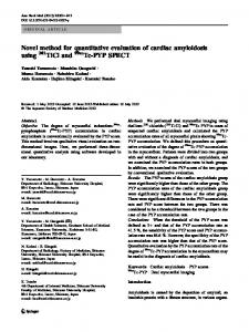
methods [24]. Figure 6 and Table 1 show the comparison results obtained from signals containing three different levels of artificial random noise (noise-free, 10%, and 20% noise) using the BN and LS regression methods, respectively. Secondly, a more complex example is studied, where the signals are collected from a multilayer sample with defects varying diameter and depth. Figure 7 illustrates the second experimental specimen (specimen number 2). The specimen consists of three layers of aluminum with a total thickness of 10 mm (2.5, 5, 2.5 mm), electrical conductivity 𝜎 = 18.5 MS/m, magnetic permeability 𝜇 = 𝜇0 = 4𝜋 × 10−7 H/m, length 420 mm, and width 80 mm. There are 5 holes with different diameters and depths in the center of
Mathematical Problems in Engineering 9
9
8
8
7
7
6
6
Diameter (mm)
Diameter (mm)
8
5 4 3
5 4 3
2
2
1
1
0
1
2
3
4 Group
5
6
0
7
1
True parameter BN LS regression
2
3
4 Group
5
6
7
True parameter BN LS regression (a)
(b)
9 8
Diameter (mm)
7 6 5 4 3 2 1 0
1
2
3
4 Group
5
6
7
True parameter BN LS regression (c)
Figure 6: The comparison of three sets of results (diameter) obtained from signals injected in three different levels of artificial random noise using BN and LS regression methods, respectively, (a) noise-free, (b) 10% noise, and (c) 20% noise (specimen number 1). Scan direction Defects diameter
X
Y
Defects depth
2.5
80 2.5
4.5
5.5
6.5
3
4
5
Z
Probe signals
2.5
5
3.5
1 50
2 80
80
80
80
50
Figure 8: The BN used in example 2 (specimen number 2). Unit: mm
Figure 7: The sketch of defects with varying diameter and depth in multilayered structures (specimen number 2).
the middle plate. The holes parameters 𝜎 = 0 S/m, 𝜇 = 𝜇0 = 4𝜋 × 10−7 H/m, diameter, and depth are (1, 2.5), (2, 3.5), (3, 4.5), (4, 5.5), and (5, 6.5) mm, respectively.
25
20
20
Normal probability density
25
15
10
15
10
5
0
Normal probability density
9
1
1.1
1.2
5
0
1.3
Diameter
2.3 Diameter
(a)
(b)
2
25
25
20
20
Normal probability density
Normal probability density
Mathematical Problems in Engineering
15
10
5
0
2.4
2.5
2.6 2.7 Diameter
2.8
2.9
3
2.1
2.2
2.4
2.5
2.6
15
10
5
0
3.3
3.4
(c)
3.5
3.6 3.7 Diameter
3.8
3.9
4.0
(d)
30
Normal probability density
25 20 15 10 5 0
5
5.2
5.4 5.6 Diameter
5.8
6
(e)
Figure 9: The estimated results (diameter) obtained from signals injected in three different levels of artificial random noise using BN method: noise-free (—), 10% noise (–⋅–), and 20% noise (. . . . . .) (specimen number 2).
10
Mathematical Problems in Engineering
25
Normal probability density
Normal probability density
20
15
10
5
0 2.5
2.6
2.7
2.8
2.9
20
15
10
5
0 3.5
3
3.6
3.8
Depth (a)
25
Normal probability density
Normal probability density
4.2
(b)
20
15
10
5
0 4.5
4 Depth
4.6
4.7
4.8 Depth
4.9
5
20
15
10
5
0
5.1
4.8
5
5.2
5.4
5.5
Depth
(c)
(d)
35
Normal probability density
30 25 20 15 10 5 0 6.5
6.6
6.7
6.8 6.9 Depth
7
7.1
(e)
Figure 10: The estimated results (depth) obtained from signals injected in three different levels of artificial random noise using BN method: noise-free (—), 10% noise (–⋅–), and 20% noise (. . . . . .) (specimen number 2).
11
6
6
5
5
4
4
Diameter (mm)
Diameter (mm)
Mathematical Problems in Engineering
3 2
2 1
1 0
3
1
2
3 Group
4
0
5
True parameter BN LS regression
1
2
3 Group
4
5
True parameter BN LS regression (a)
(b)
6
Diameter (mm)
5 4 3 2 1 0
1
2
3 Group
4
5
True parameter BN LS regression (c)
Figure 11: The comparison of three sets of results (diameter) obtained from signals injected in three different levels of artificial random noise using BN and LS regression methods, respectively, (a) noise-free, (b) 10% noise, and (c) 20% noise (specimen number 2).
In this example, the random variables are the defect diameter X, defect depth Y, and the probe response signals Z. The defect diameter and depth are two independent influencing factors of the probe signals. Using this special relationship, we can obtain the BN structure given in Figure 8. Node X and node Y are linked to node Z by an arc, respectively. Like the first example, the distributions of X, Y, and Z are also assumed as multivariate Gaussian with unknown means and variances. In the experiment, a dataset with 150 records is acquired during scanning. The dataset contains EC signals from 5 types
of defects (each type having 30 records). As described in the previous experiments, the same procedures are carried out. The diameter and depth estimation results obtained from signals containing three different levels of artificial random noise (noise-free, 10%, and 20% noise) using the BN method are shown in Figures 9 and 10, respectively. The comparison results of the estimated diameter and depth obtained from signals containing three different levels of artificial random noise (noise-free, 10%, and 20% noise) using the BN and LS regression methods are shown in Figures 11 and 12 and Table 2, respectively.
12
Mathematical Problems in Engineering 8 7
Depth (mm)
6 5 4 3 2 1 0
1
2
3 Group
4
5
1
2
True parameter BN LS regression
8
8
7
7
6
6
5
5
Depth (mm)
Depth (mm)
(a)
4 3
4 3
2
2
1
1
0
1
2
3 Group
4
5
True parameter BN LS regression
0
3 Group
4
5
True parameter BN LS regression (b)
(c)
Figure 12: The comparison of three sets of results (depth) obtained from signals injected in three different levels of artificial random noise using BN and LS regression methods, respectively, (a) noise-free, (b) 10% noise, and (c) 20% noise (specimen number 2).
Tables 1 and 2 show quantitatively the estimation error and the corresponding methods. It can be seen that the BN method has a higher precision than the LS regression method. The LS regression method has difficulty performing more accurate estimation and the satisfactory solution becomes unlikely in the case of signals containing high-level noise. In contrast, the BN method can achieve greater accuracy and robustness, even in the case of signals containing highlevel noise. It provides not only the accurate estimation of defect characteristic parameters, but also the probability distributions of these values. With increasing noise level,
the estimated variances also increase, whereas the estimated means deviations from their actual values increase very limitedly. This demonstrates that although the variances growth means increasing the uncertainty of the results, the estimated error of BNs increases only slightly with the increasing noise level. It shows that BNs are effective in the quantitative evaluation of defects, due to their remarkable characteristics such as the combination of the domain knowledge and the reasoning under uncertainty in AI. This eventually results in better generalization performance in the BN method than the LS regression method. In brief, the BN method is able to
Mathematical Problems in Engineering
13
Table 1: Defect parameter estimation errors obtained by the BN method and the LS method (specimen number 1).
Diameter error (RMSE)
Signals Noise-free 10% noise 20% noise
LS 0.6465 0.6761 0.7556
BN 0.2597 0.3119 0.3915
Table 2: Defect parameter estimation errors obtained by the BN method and the LS method (specimen number 2).
Diameter error (RMSE)
Depth error (RMSE)
Signals Noise-free 10% noise 20% noise Noise-free 10% noise 20% noise
LS 0.6596 0.6918 0.7271 0.7050 0.7942 0.8893
BN 0.2813 0.3709 0.4464 0.3213 0.4140 0.4944
successfully cope with highly complex and ill-posed ECNDE inverse problems, where each defect is hidden deeply in a multilayered structure.
(Gamma, Poisson, etc.). BNs can handle the problem where each conditional distribution of each variable can be any distributions. However, these possibilities are out of the scope of this paper and are the topic of current and future work of the authors. It will be helpful to analyze the EC signals more accurately in detail and lead to more precise predictions. In addition, it is necessary to note that, in this paper, the problem under investigation is simple. However, in most ECNDT problems, the more complex configuration (interacting defects, partially conducting defects, defects with nonregular shape as corrosions, real defects, etc.) is to be handled. Future work, hopefully, will be done to extend the proposed BN method to the more complex ECNDT problems where the more unknown parameters of defects need to be estimated. We consider that the independence of causal influence can be exploited in Bayesian networks to reduce both the time and space cost of inference. The increase of the computational costs with the increase of the unknown parameters is the computation of the decomposed additional local joint probability density inference.
Conflict of Interests The authors declare that there is no conflict of interests regarding the publication of this paper.
5. Conclusions A new approach for quantitative evaluation of defects in multilayered structures from ECNDT signals using BNs has been proposed and investigated. BNs discussed in this paper are simple and powerful, and their structures and parameters are easily learned from the domain knowledge of ECNDT and experimental data. The generative model can predict the probe response signals given the defect characteristic parameters or estimate the defect characteristic parameters from the inspection signals by using probability inference. In this paper, we mainly describe how the problem of defect characteristic parameter estimation from ECNDT signals can be modeled using BNs, in which the general model accommodates the uncertainties of the EC inspection. Two experiments have been carried out. Compared with the LS regression method, BNs have the advantage of being a bidirectional inferential mechanism and higher accuracy and robustness. They allow results to be obtained in the form of full CPDs, accounting for all the information available (evidences). It can be seen that the estimation results are probabilities rather than a single value. More information about the estimated parameters can be deduced from their probabilities, such as the means and variances, which describe the value itself and the degree of uncertainty respectively. The experimental results demonstrate the feasibility and effectiveness of the BN method proposed in this paper. This also encourages the attempts to tackle the other evaluation problems. In this paper, the multivariate Gaussian assumption of all variables has been taken. Nevertheless, in real problems where the distributions are nonuniform, a non-Gaussian assumption also could be more suitable. In fact, the validity of BNs is not restricted to the particular case of multivariate Gaussian distributions but to more general distributions
Acknowledgment This work is supported by the National Natural Science Foundation of China Grant nos. 51105183 and 51307172, the Research Fund for the Doctoral Program of Higher Education of China Grant no. 20115314120003, the Applied Basic Research Programs of Science and Technology Commission Foundation of Yunnan Province of China Grant no. 2010ZC050, the Foundation of Yunnan Educational Committee Grant no. 2013Z121, the National College Student Innovation Training Program Funded Projects Grant no. 201210674014, and the Science and Technology Project of Yunnan Power Grid Corporation Grant no. K-YN2013-110.
References [1] B. A. Auld and J. C. Moulder, “Review of advances in quantitative eddy current nondestructive evaluation,” Journal of Nondestructive Evaluation, vol. 18, no. 1, pp. 3–36, 1999. [2] H. Zhang, H. C. Yan, F. W. Yang, and Q. J. Chen, “Quantized control design for impulsive fuzzy networked systems,” IEEE Transactions on Fuzzy Systems, vol. 19, no. 6, pp. 1153–1162, 2011. [3] N. Meyendorf and A. Berthold, “New trends in NDE and health monitoring,” in Advanced Sensor Technologies for Nondestructive Evaluation and Structural Health Monitoring II, vol. 6179 of Proceedings of SPIE, pp. 617901–617910, San Diego, Calif, USA, March 2006. [4] F. Kojima and T. Fujioka, “Quantitative evaluation of material degradation parameters using nonlinear magnetic inverse problems,” International Journal of Applied Electromagnetics and Mechanics, vol. 25, no. 1–4, pp. 157–163, 2007. [5] K. Chomsuwan, S. Yamada, and M. Iwahara, “Improvement on defect detection performance of PCB inspection based on ECT
14
[6]
[7]
[8]
[9]
[10]
[11]
[12]
[13] [14]
[15]
[16]
[17]
[18]
[19]
[20]
[21]
[22]
Mathematical Problems in Engineering technique with multi-SV-GMR sensor,” IEEE Transactions on Magnetics, vol. 43, no. 6, pp. 2394–2396, 2007. J. H. Cantrell and W. T. Yost, “Nonlinear ultrasonic characterization of fatigue microstructures,” International Journal of Fatigue, vol. 23, supplement 1, pp. S487–S490, 2001. H. Nˇemec, P. Kuˇzel, F. Garet, and L. Duvillaret, “Time-domain terahertz study of defect formation in one-dimensional photonic crystals,” Applied Optics, vol. 43, no. 9, pp. 1965–1970, 2004. M. R. Clark, D. M. McCann, and M. C. Forde, “Application of infrared thermography to the non-destructive testing of concrete and masonry bridges,” NDT and E International, vol. 36, no. 4, pp. 265–275, 2003. T. Toutountzakis and D. Mba, “Observations of acoustic emission activity during gear defect diagnosis,” NDT and E International, vol. 36, no. 7, pp. 471–477, 2003. H. Elaqra, N. Godin, G. Peix, M. R’Mili, and G. Fantozzi, “Damage evolution analysis in mortar, during compressive loading using acoustic emission and X-ray tomography: effects of the sand/cement ratio,” Cement and Concrete Research, vol. 37, no. 5, pp. 703–713, 2007. Y. Bar-Cohen, “Emerging NDT technologies and challenges at the beginning of the third millennium, part 1,” Materials Evaluation, vol. 58, no. 1, pp. 17–30, 2000. Y. Bar-Cohen, “Emerging NDT technologies and challenges at the beginning of the third millennium, part 2,” Materials Evaluation, vol. 58, no. 2, pp. 141–150, 2000. S. J. Norton and J. R. Bowler, “Theory of eddy current inversion,” Journal of Applied Physics, vol. 73, no. 2, pp. 501–512, 1993. H. J. Gao, T. W. Chen, and J. Lam, “A new delay system approach to network-based control,” Automatica, vol. 44, no. 1, pp. 39–52, 2008. J. P´av´o, “Approximate methods for the calculation of the ECT signal of a crack in a plate coated by conducting deposit,” IEEE Transactions on Magnetics, vol. 40, no. 2, pp. 659–662, 2004. A. Sophian, G. Y. Tian, D. Taylor, and J. Rudlin, “Electromagnetic and eddy current NDT: a review,” Insight: Non-Destructive Testing and Condition Monitoring, vol. 43, no. 5, pp. 302–306, 2001. H. Zhang, H. C. Yan, F. W. Yang, and Q. J. Chen, “Distributed average filtering for sensor networks with sensor saturation,” IET Control Theory & Applications, vol. 7, no. 6, pp. 887–893, 2013. O. Bottauscio, M. Chiampi, and A. Manzin, “Eddy current problems in nonlinear media by the element-free Galerkin method,” Journal of Magnetism and Magnetic Materials, vol. 304, no. 2, pp. e823–e825, 2006. T. Dogaru, C. H. Smith, R. W. Schneider, and S. T. Smith, “Deep crack detection around fastener holes in airplane multi-layered structures using GMR-based eddy current probes,” in Quantitative Nondestructive Evaluation, vol. 23 of AIP Conference Proceedings, pp. 398–405, Green Bay, Wis, USA, July-August 2004. E. Cardelli, A. Faba, R. Specogna, A. Tamburrino, F. Trevisan, and S. Ventre, “Analysis methodologies and experimental benchmarks for eddy current testing,” IEEE Transactions on Magnetics, vol. 41, no. 5, pp. 1380–1383, 2005. P. G. Kaup, F. Santosa, and M. Vogelius, “Method for imaging corrosion damage in thin plates from electrostatic data,” Inverse Problems, vol. 12, no. 3, pp. 279–293, 1996. B. Ye, G. Zhang, P. Huang, M. Fan, S. Zheng, and Z. Zhou, “Quantifying geometry parameters of defect in multi-layered
[23]
[24]
[25]
[26]
[27]
[28]
[29] [30]
[31] [32] [33]
[34]
[35]
[36] [37]
[38]
[39]
structures from eddy current nondestructive evaluation signals by using genetic algorithm,” in Proceedings of the 6th World Congress on Intelligent Control and Automation, vol. 2, pp. 5358– 5362, Dalian, China, June 2006. I. T. Rekanos, T. P. Theodoulidis, S. M. Panas, and T. D. Tsiboukis, “Impedance inversion in eddy current testing of layered planar structures via neural networks,” NDT and E International, vol. 30, no. 2, pp. 69–74, 1997. H. C. Yan, Z. Z. Su, H. Zhang, and F. W. Yang, “Observerbased 𝐻∞ control for discrete-time stochastic systems with quantisation and random communication delays,” IET Control Theory & Applications, vol. 7, no. 3, pp. 372–379, 2013. J. I. de la Rosa, G. A. Fleury, S. E. Osuna, and M. E. Davoust, “Markov chain Monte Carlo posterior density approximation for a groove-dimensioning purpose,” IEEE Transactions on Instrumentation and Measurement, vol. 55, no. 1, pp. 112–122, 2006. H. C. Yan, H. B. Shi, H. Zhang, and F. W. Yang, “Quantized 𝐻∞ control for networked systems with communication constraints,” Asian Journal of Control, vol. 15, no. 5, pp. 1468–1476, 2013. T. Khan and P. Ramuhalli, “A recursive bayesian estimation method for solving electromagnetic nondestructive evaluation inverse problems,” IEEE Transactions on Magnetics, vol. 44, no. 7, pp. 1845–1855, 2008. J. Pearl, Probabilistic Reasoning in Intelligent Systems: Networks of Plausible Inference, The Morgan Kaufmann Series in Representation and Reasoning, Morgan Kaufmann, San Mateo, Calif, USA, 1988. D. Heckerman, “A tutorial on learning Bayesian networks,” Tech. Rep. MSR-TR-95-06, Microsoft Research, 1995. A. Kameari, “Three dimensional eddy current calculation using finite element method with A-V in conductor and in vacuum,” IEEE Transactions on Magnetics, vol. 24, no. 1, pp. 118–121, 1987. S. J. Norton and J. R. Bowler, “Theory of ECT inversion,” Journal of Applied Physics, vol. 73, no. 2, pp. 501–512, 1993. J. Gill, Bayesian Methods: A Social and Behavioral Sciences Approach, Chapman & Hall/CRC, Boca Raton, Fla, USA, 2002. E. Castillo, J. M. Guti´errez, and A. S. Hadi, Expert Systems and Probabilistic Network Models, Springer, New York, NY, USA, 1997. H. Zhang, H. C. Yan, T. Liu, and Q. J. Chen, “Fuzzy controller design for nonlinear impulsive fuzzy systems with time delay,” IEEE Transactions on Fuzzy Systems, vol. 19, no. 5, pp. 844–856, 2011. F. V. Jensen, Bayesian Networks and Decision Graphs, Statistics for Engineering and Information Science, Springer, New York, NY, USA, 2001. C. R. Kenley, Influence diagram models with continuous variables [Ph.D. thesis], Stanford University, Stanford, Calif, USA, 1986. D. Heckerman, D. Geiger, and D. M. Chickering, “Learning Bayesian networks: the combination of knowledge and statistical data,” Machine Learning, vol. 20, no. 3, pp. 197–243, 1995. H. Zhang, Q. J. Chen, H. C. Yan, and J. H. Liu, “Robust 𝐻∞ filtering for switched stochastic system with missing measurements,” IEEE Transactions on Signal Processing, vol. 57, no. 9, pp. 3466–3474, 2009. I. Cohen, N. Sebe, F. G. Gozman, M. C. Cirelo, and T. S. Huang, “Learning Bayesian network classifiers for facial expression recognition both labeled and unlabeled data,” in Proceedings of the IEEE Computer Society Conference on Computer Vision and Pattern Recognition, vol. 1, pp. I-595–I-601, June 2003.
Mathematical Problems in Engineering [40] C. Meek, “Causal inference and causal explanation with background knowledge,” in Proceedings of the 11th Annual Conference on Uncertainty in Artificial Intelligence (UAI ’95), pp. 403–410, 1995. [41] H. Zhang, Z. H. Guan, and G. Feng, “Reliable dissipative control for stochastic impulsive systems,” Automatica, vol. 44, no. 4, pp. 1004–1010, 2008. [42] L. X. Zhang, H. J. Gao, and O. Kaynak, “Network-induced constraints in networked control systems—a survey,” IEEE Transactions on Industrial Informatics, vol. 9, no. 1, pp. 403–416, 2013. [43] C. Huang and A. Darwiche, “Inference in belief networks: a procedural guide,” International Journal of Approximate Reasoning, vol. 15, no. 3, pp. 225–263, 1996. [44] P. Huang, G. Zhang, Z. Wu, J. Cai, and Z. Zhou, “Inspection of defects in conductive multi-layered structures by an eddy current scanning technique: simulation and experiments,” NDT and E International, vol. 39, no. 7, pp. 578–584, 2006. [45] R. O. Duda, P. E. Hart, and D. G. Stork, Pattern Classification, John Wiley & Sons, New York, NY, USA, 2nd edition, 2001.
15
Advances in
Operations Research Hindawi Publishing Corporation http://www.hindawi.com
Volume 2014
Advances in
Decision Sciences Hindawi Publishing Corporation http://www.hindawi.com
Volume 2014
Journal of
Applied Mathematics
Algebra
Hindawi Publishing Corporation http://www.hindawi.com
Hindawi Publishing Corporation http://www.hindawi.com
Volume 2014
Journal of
Probability and Statistics Volume 2014
The Scientific World Journal Hindawi Publishing Corporation http://www.hindawi.com
Hindawi Publishing Corporation http://www.hindawi.com
Volume 2014
International Journal of
Differential Equations Hindawi Publishing Corporation http://www.hindawi.com
Volume 2014
Volume 2014
Submit your manuscripts at http://www.hindawi.com International Journal of
Advances in
Combinatorics Hindawi Publishing Corporation http://www.hindawi.com
Mathematical Physics Hindawi Publishing Corporation http://www.hindawi.com
Volume 2014
Journal of
Complex Analysis Hindawi Publishing Corporation http://www.hindawi.com
Volume 2014
International Journal of Mathematics and Mathematical Sciences
Mathematical Problems in Engineering
Journal of
Mathematics Hindawi Publishing Corporation http://www.hindawi.com
Volume 2014
Hindawi Publishing Corporation http://www.hindawi.com
Volume 2014
Volume 2014
Hindawi Publishing Corporation http://www.hindawi.com
Volume 2014
Discrete Mathematics
Journal of
Volume 2014
Hindawi Publishing Corporation http://www.hindawi.com
Discrete Dynamics in Nature and Society
Journal of
Function Spaces Hindawi Publishing Corporation http://www.hindawi.com
Abstract and Applied Analysis
Volume 2014
Hindawi Publishing Corporation http://www.hindawi.com
Volume 2014
Hindawi Publishing Corporation http://www.hindawi.com
Volume 2014
International Journal of
Journal of
Stochastic Analysis
Optimization
Hindawi Publishing Corporation http://www.hindawi.com
Hindawi Publishing Corporation http://www.hindawi.com
Volume 2014
Volume 2014