A Bayesian sampling approach to measuring the price responsiveness of gasoline demand using a constrained partially linear model Haotian Chen† , †
Russell Smyth‡ 1 ,
Xibin Zhang†
Department of Econometrics and Business Statistics, Monash University, Australia ‡
Department of Economics, Monash University, Australia August 26, 2016
Abstract. Partial linear models provide an intuitively appealing way to examine gasoline demand because one can examine how response to price varies according to the price level and people’s income. However, despite their intuitive appeal, partial linear models have tended to produce implausible and/or erratic price effects. Blundell et al. (2012) propose a solution to this problem that involves using Slutsky shape restrictions to improve the precision of the nonparametric estimate of the demand function. They propose estimating a constrained partially linear model through three steps, where the weights are optimized by minimizing an objective function under the Slutsky constraint, bandwidths are selected through least squares cross-validation, and linear coefficients are estimated using profile least squares. A limitation of their three-step estimation method is that bandwidths are selected based on pre-estimated parameters. We improve on the Blundell et al. (2012) solution in that we derive a posterior and develop a posterior simulation algorithm to simultaneously estimate the linear coefficients, bandwidths in the kernel estimator and the weights imposed by the Slutsky condition. With our proposed sampling algorithm, we estimate a constrained partially linear model of household gasoline demand employing household survey data for the United States for 1991 and 2001 and find plausible price effects. Keywords: Kernel estimator; Markov chain Monte Carlo; Price elasticity; Slutsky condition; Smoothness JEL Classification: C14; C11; D12; H31
1 Address: 20 Chancellors Walk, Wellington Road, Clayton, VIC 3800, Australia. Telephone: +61 3 99051560. Fax: +61 3 99055476. Email:
[email protected].
1
1 Introduction Estimating the demand for gasoline is an important research topic given the growth in motor vehicle ownership and resultant environmental implications of carbon dioxide emissions from this source. Of particular concern to policy makers is the effect of price changes on gasoline demand. The responsiveness of motor vehicle users to rises in the price of gasoline dictates the extent to which governments can impose taxes in order to raise revenue, encourage conservation through discouraging demand for gasoline and encouraging switching in favour of cleaner fuel sources, as well as attain certain national security objectives in terms of energy independence (see Dahl, 1979; Dahl and Sterner, 1991; Goel, 1994; Hausman and Newey, 1995; Deaton and Paxson, 1998; Manzan and Zerom, 2010; Chang and Serletis, 2014). As a consequence, a large literature has evolved that seeks to estimate the price elasticity of gasoline demand in order to inform policymakers. Much of this uses aggregate data, although some uses household-level data (see for example, Dahl and Sterner, 1991; Graham and Glaister, 2002; Brons et al., 2008; Espey, 1998; Havranek et al., 2012, for surveys). Economic theory provides no specific guidance on the appropriate functional form for the gasoline demand function. Most analyses of gasoline demand employs some form of parametric specification, such as linear, log-linear or translog and assume the distribution of the error term to be normal with zero mean and fixed variance. The results from such models are easy to interpret because parametric modelling gives constant price and income elasticities. For ‘representative consumers’, parametric modelling of gasoline demand mostly suggests that gasoline demand is price inelastic. Meta-analyses suggest that the long-run price elasticity is in the range −0.31 (Havranek et al., 2012) to −0.84 (Espey, 1998). However, the problem is that it will often be inappropriate to assume that demand elasticities are constant across groups of consumers with different incomes and facing different prices. As Hausman and Newey (2016, p.1125) have recently emphasised: “Demand functions could vary across individuals in general ways”. Parametric specifications are not well suited to study potential variation in the elasticity of demand, although understanding how people’s response to price varies according to the price level, and across the income distribution, is of importance to policymakers (Blundell et al., 2012).
2
In such circumstances, using a partial linear model is an attractive solution to model household gasoline demand if we believe that the relationship between some independent variables and gasoline are linear, while the relationship between other independent variables and gasoline are non-linear. In response, beginning with Hausman and Newey (1995), there has been growing interest in modelling gasoline demand through applying semi-parametric models to household survey data (see for example, Schmalensee and Stoker, 1999; Yatchew and No, 2001; Coppejans, 2003; Blundell et al., 2012; Manzan and Zerom, 2010; Wadud et al., 2010b; Liu, 2014). Yet, while estimating partial linear models with household data seems intuitively attractive, as Blundell et al. (2012) have noted, nonparametric and semi-parametric regression can yield implausible and erratic estimates. A feature of much of the earlier literature to estimate gasoline demand with semi-parametric regression is that it found erratic price effects. For example, using household survey data for the United States (US), Hausman and Newey (1995) and Schmalensee and Stoker (1999) found that as price increases, the fitted demand curve exhibits an upward slope when the price is within a middle range and a downward slope elsewhere. Moreover, Schmalensee and Stoker (1999) found that the average derivative of the estimated demand with respect to price is positive. These findings contradict conventional consumer theory, which implies that gasoline demand should decrease as gasoline price increases. There continues to be substantial differences in the more recent semi-parametric regression literature regarding estimates of the price elasticity of gasoline in the US (see for example, Blundell et al., 2012; Manzan and Zerom, 2010; Hausman and Newey, 2016). Blundell et al. (2012) suggested that erratic and/or implausible price effects with semiparametric regression reflect imprecision of the unconstrained semi-nonparametric estimates. Their solution to this problem was to impose the Slutsky condition on the kernel estimator of the nonlinear component, through which gasoline price and household income effect gasoline demand. Fitting a constrained partially linear model to US household survey data for 2001, they found an inverse relationship between gasoline price and demand, consistent with consumer theory. A practical limitation of their solution, though, is that estimation of this constrained model is complicated because the vector of weights imposed by the Slutsky condition has a dimension equal to the sample size. Hence, the total number of unknown identities including 3
coefficients, bandwidths and weights is larger than the sample size. Blundell et al. (2012) suggested estimating this constrained partially linear model through three steps, where the weights are optimized by minimizing an objective function under the Slutsky constraint, bandwidths are selected through least squares cross-validation, and linear coefficients are estimated using the profile least squares method discussed by Speckman (1988) and Robinson (1988). To the best of our knowledge, no method is available to simultaneously estimate the linear coefficients, bandwidths and weights imposed by the Slutsky condition. We fill this gap in the literature through proposing such a method and present a sampling approach to the estimation of a partially linear model subject to the Slutsky condition. We propose a methodological improvement to the manner in which partial linear models are used to estimate household gasoline demand and illustrate our contribution through estimating household gasoline demand using US survey data. Our starting point is that price elasticity, which is computed through the first derivative of the fitted demand with respect to price, depends on the smoothness of the kernel estimator of the nonlinear function, through which price and income effect demand. The performance of this kernel estimator is mainly determined by bandwidths (see, for example, Härdle, 1990). Schmalensee and Stoker’s (1999) finding of an implausible price effect is likely to be due to the lack of Slutsky constraint on the kernel estimator and a subjective choice of bandwidths. Blundell et al. (2012) introduced such a constraint, but a limitation of their three-step estimation method is that bandwidths are selected based on pre-estimated parameters. We improve on the approach adopted by Blundell et al. (2012) in that we derive a posterior and develop a posterior simulation algorithm to simultaneously estimate the linear coefficients, bandwidths in the kernel estimator and the weights imposed by the Slutsky condition. Specifically, we contribute to the literature on estimating partial linear models of household gasoline demand with survey data in the following important ways: • We derive a posterior for the partially linear model with its kernel estimator of the nonlinear component being subject to the Slutsky condition. A Markov chain Monte Carlo (MCMC) sampling algorithm is developed to simultaneously sample linear coefficients
4
and bandwidths, as well as the weights imposed by the Slutsky condition. • With the proposed sampling algorithm, we estimate the constrained partially linear model of household gasoline demand employing the same 1991 US survey data as originally employed by Schmalensee and Stoker (1999) and find, contrary to their result, that the price elasticity for household gasoline demand is negative. • With the proposed sampling algorithm, we also estimate the constrained partially linear model of household gasoline demand employing the 2001 US survey data used by Blundell et al. (2012). We find not only a negative price effect, which is largely consistent with Blundell et al.’s (2012) finding, but, contrary to their findings, that middle-and high-income earners are less sensitive to gasoline price increases, while low-income households are more sensitive to gasoline price changes. The rest of this paper is organized as follows. In the next section, we present the posterior for a partially linear model with its kernel estimator of the nonlinear component being subject to the Slutsky constraint. We also present a sampling algorithm. In Section 3, we apply this sampling procedure to estimate constrained partially linear models for household gasoline demand and examine the relevant price effects. To do so, we use data from the 1991 and 2001 US household transportation surveys, which facilitate comparison between our results and those in Schmalensee and Stoker (1999) and Blundell et al. (2012). Section 4 concludes the paper and draws out the broader advantages of our approach for modeling gasoline demand.
2 A partially linear model subject to the Slutsky condition 2.1 Model and posterior Suppose that a response variable y can be explained by x and z in the form of y = x0 β + g (z ) + ε,
(1)
where β is a d × 1 vector of unknown parameters, and g (·) is an unknown nonlinear function ¡ ¢0 with its argument being either a scalar or a vector. Let y i , x0i , zi , for i = 1, 2, · · · , n, denote obser5
vations of (y , x0 , z )0 . It is also assumed that the error terms εi , for i = 1, 2, · · · , n, are independent and identically distributed (iid) with an unknown density f (ε). Let z = (z 1 , z 2 )0 and zi = (z 1i , z 2i )0 , where z 1 and z 2 are the price and income variables in the household data of gasoline demand. In the partially linear model (1), g (z ) is estimated by a weighted Nadaraya-Watson (NW) estimator. It is a function of price and household income and is expressed as (Hall and Huang, 2001; Blundell et al., 2012) ¡ ¢¡ ¢ Pn 0 ¡ ¢ j =1 w j K h zi − z j y j − x j β ¡ ¢ gb zi |h = , P n −1 nj=1 K h zi − z j
(2)
for i = 1, 2, · · · , n, where w 1 , w 2 , · · · , w n are non-negative weights, and K h (·) is a kernel function with bandwidths h. In this paper, we use the normal kernel, φ(·/h)/h. When the argument of g (·) is multivariate, the kernel function is the product of normal kernels with different bandwidths being assigned to different variables. Once the kernel function is chosen, the weighted NW estimator is determined by its bandwidths. In order to ensure consistency with consumer theory, Blundell et al. (2012) imposed the Slutsky constraint to evaluate the price effect based on g (z ) in (1). The Slutsky constraint is expressed as ¡ ∂gb(z 1 , z 2 ) ∂gb(z 1 , z 2 ) + gb z 1 , z 2 ) ≤ 0. ∂z 1 ∂z 2
(3)
According to Hall and Huang (2001) and Blundell et al. (2012), this constraint can be achieved by minimizing an objective function given by D(w 1 , · · · , w n ) = n −
n X
(nw i )1/2 ,
(4)
i =1
where w i ≥ 0, for i = 1, 2, · · · , n, and
Pn
i =1 w i
= 1.
In order to choose the bandwidth for the weighted NW estimator, we use the leave-more-out NW estimator, which requires us to exclude the j th observation that makes z j − zi = 0 in the weighted NW estimator given by (2). Let © ª J i = j : z j 6= zi , for j = 1, 2, · · · , n , ¡ ¢ for i = 1, 2, · · · , n, and let n i be the number of observations excluded from gb zi |h . 6
The leave-more-out NW estimator is given by ¢ ¡ ¢¡ w ∗j K h zi − z j y j − x 0j β ¡ ¢ , P (n − n i )−1 j ∈J i K h zi − z j
P ¡
¢
gb(i ) zi |h =
j ∈J i
where w ∗j , for j ∈ J i , are the weights satisfying
P
j ∈J i
(5)
w ∗j = 1, for i = 1, 2, · · · , n. Therefore, we
re-weight the original weights as w ∗j =
wj n − ni
,
with j ∈ J i , for i = 1, 2, · · · , n. The purpose of excluding the kernel functions with a zero argument out of these two summations is to avoid undesirable values of bandwidths. With a sample of n observations of (y , x0 , z ) for model (1), we assume that the errors, ε1 , ε2 , · · · , εn , are independent and identically distributed with a kernel-form density discussed by Zhang and King (2013): f (ε|σ) =
n 1 ³ε−ε ´ 1 X j φ , n j =1 σ σ
(6)
where φ(·) is the standard Gaussian density function with σ being its standard deviation, which serves as a smoothing parameter, also known as the bandwidth. To choose bandwidth for this kernel-form density of errors, we use its leave-one-out version: ¡ ¢ f εi |σ =
n 1 ³ε −ε ´ 1 X i j φ , n − 1 j =1 σ σ
(7)
j 6=i
where εi = y i − x0i β − g (zi ), for i = 1, 2, · · · , n. In the partially linear model given by (1), if g (z ) were unknown, the density of y i would be ª © ¡ ¢ª! é 0 0 n y − x β − g z − y − x β − g zj ( ) X i i j ¡© ª¯ ¢ 1 1 i j y i ∼ f y i − x i0 β − g (zi ) ¯σ = φ . (8) n − 1 j =1 σ σ j 6=i
¡ ¢ As g (zi ) is unknown, it is approximated by gb(i ) zi |h , for i = 1, 2 · · · , n. Therefore, we have yi ∼ f
¡©
¢ª¯ ¢ y i − x i0 β − gbi zi |h ¯σ = ¡
n 1 1 X φ n − 1 j =1 σ
é
¡ ¢ª © ¡ ¢ª ! y i − x i0 β − gb(i ) zi |h − y j − x 0j β − gb( j ) z j |h σ
j 6=i
for i = 1, 2, · · · , n.
7
,
We treat the squared bandwidths h2 and σ2 as parameters and denote the parameter vector ¡ ¢0 ¡ ¢0 as θ = β0 , w , h2 , σ2 . The likelihood of y = y 1 , y 2 , · · · , y n given θ is approximately n ¡ ¢ Y ¡© ¡ ¢ª¯ ¢ L y |θ = f y i − x i0 β − gb(i ) zi |h ¯σ , i =1 n Y
n 1 1 X φ = n − 1 j =1 σ i =1
é
y i − x i0 β − gb(i )
¡ ¢ª ¢ª © ! zi |h − y j − x 0j β − gb( j ) z j |h
¡
σ
j 6=i
.
(9)
2.2 Priors and posterior The prior of β is assumed to be a normal density with mean β0 and variance-covariance V0 , which are hyperparameters. We assume that the priors of h 2 and σ2 are the inverse Gamma density expressed as α
λh h
¶αh +1
½ ¾ λh exp − 2 , h
(10)
µ ¶ασ +1 ½ ¾ α ¡ 2¢ λσσ 1 λσ πσ = exp − 2 , Γ(ασ ) σ2 σ
(11)
πh ¡
2
¢
µ
1 = Γ(αh ) h 2
and
where λh , αh , λσ and ασ are hyperparameters. We assume that the proposal density q(w i ) for i = 1, 2, · · · , n, is a Dirichlet density q(w i ) ∼ Dir(ξ), with a hyperparameter ξ. The joint prior of θ is the product of these marginal priors and is denoted as π(θ). By Bayes theorem, the posterior of θ is (up to a normalizing constant) π(θ|y ) ∝ π(θ) × L(y |θ),
(12)
from which we sample θ through the random-walk Metropolis algorithm described as follows. ³ ´0 2 Step 1: Randomly choose feasible initial values denoted as β(0) , h (0) , σ2(0) , w(0) . ³ ´0 2 Step 2: Conditional on h (0) , σ2(0) , w(0) , we use the random-walk Metropolis algorithm to sample β subject to the constraint (3) and denote the update as β(1) . 8
³ ´0 Step 3: Conditional on β(1) , σ2(0) , w(0) , we use the random-walk Metropolis algorithm to sam2 ple h 2 subject to the constraint (3) and denote the update as h (1) .
³ ´0 2 Step 4: Conditional on β(1) , h (1) , w(0) , we use the random-walk Metropolis algorithm to sample σ2 and denote the update as σ2(1) . ³ ´0 2 , σ2(1) , we use the independent Metropolis-Hastings algorithm Step 5: Conditional on β(1) , h (1) to sample w as follows. i) Generate w from Dir(ξ) and denote it as w b , which is a proposal for the next state of w . ii) Compute the target function D(w b ) in (4). Accept the proposal if D(w b ) > D(w (i ) ). iii) Otherwise, compute the acceptance probability: ³ ´ D(w b )q(w (i ) ) . A w (i ) , w b = D(w (i ) )q(w b) © ¡ ¢ª b . iv) Accept the proposal with the probability given by min 1, A w (i ) , w Step 6: Repeat Steps 2 – 5 until the chain
n³
´0 o β(i ) , h (i2 ) , σ2(i ) , w(i ) : i = 1, 2, · · · achieves reasonable
mixing performance.
3 Partially linear models of household gasoline demand 3.1 Data Our study is based on the data sets collected through the Residential Transportation Energy Demand Survey (RTECS) in 1991 and the National Household Travel Survey (NHTS) in 2001. In each data set, we filtered the data by retaining those individuals with non-zero values of gallons consumed, miles driven, number of licensed drivers and number of cars owned. Therefore, there are 2697 individuals in the sample of the 1991 survey, and 5254 individuals in the sample of the 2001 survey. The 1991 data contains 26 variables, 21 of which are dummy variables of region, type of residence and life cycle phase. The 2001 data contains 21 variables, 14 of which are dummy variables of region, type of residence and public transit indicator. We present a brief description and a summary of descriptive statistics of these variables in Tables 1 and 2. 9
Our study is focused on the price effect of household gasoline demand at different income levels. In the 1991 survey data sample, income data were organized into four groups, which are the low-income group at $12,000, middle-income group at $20,000, high-income group at $35,000 and higher-income group at $70,000. In the 2001 survey data sample, we have three income levels, which are the low-income group at $42,500, middle-income group at $57,500 and high-income group at $72,500. When estimating bandwidths and parameters, we allow different bandwidths and parameters for different income groups, each of which contains income data within 50% of the income level. Thus, our estimation differs from Schmalensee and Stoker’s (1999) estimation, which uses the whole sample of the 1991 survey to estimate parameters.
3.2 A model of household gasoline demand and elasticity measures Blundell et al. (2012) used a constrained partially linear model to study how household gasoline demand is affected by household income, driver’s age, gasoline price and other variables. This type of model is expressed as ¡ ¢ y i = x0i β + g z 1i , z 2i + εi ,
(13)
for i = 1, 2, · · · , n, where y i is the log of gasoline demand, z 1i and z 2i are log of price and log of income, xi is a vector explanatory variables, and εi , for i = 1, 2, · · · , n, are iid errors. The nonlinear function was estimated through the constrained NW estimator given by (2). For the price variables in the nonlinear component of (13), we computed price elasticities at a set of points of price variables using a direct derivative estimator: ¢¯ ∂ ¡ δbi = gb z 1 , z 2 ¯z=zi , ∂z 1 where z 2 are fixed income values for each income group.
3.3 Price effect on gasoline demand based on the 1991 survey data An important finding of Schmalensee and Stoker (1999) based on the 1991 survey data is that the price effect is implausible because their estimated price elasticity is positive. They argued that such an unreasonable estimate is due to the unreliability of the price data. Following 10
Schmalensee and Stoker’s (1999) variable selection, we chose log age, log number of drivers, log household size, residence and life cycle dummy variables to linearly explain gasoline demand in the model given by (13).2 In terms of the choices of hyperparameters, the mean vector and variance-covariance matrix of the normal prior density of β are respectively, chosen to be 0 and 25I with 0 being a vector of zeros and I being the identity matrix. Hyperparameters of the inverse Gamma prior are chosen to be αh = ασ = 1 and λh = λσ = 0.05, and the hyperparameter of the Dirichlet prior is chosen as ξ = 1. Estimation results are presented in Table 3, where each parameter is estimated by the arithmetic mean of the corresponding simulated chain, and values in parentheses are the corresponding 95% Bayesian credible intervals. For the low-, middle-, high- and higher-income groups, the bivariate vectors of bandwidths, which are assigned to log price and log income in the constrained kernel estimator, are estimated as (0.1217, 1.3461), (0.1172, 1.3155), (0.1202, 1.3509) and (0.1206, 1.3170), respectively. In contrast, Schmalensee and Stoker (1999) subjectively chose the two bandwidths as 0.3. This indicates that their bandwidths might lead to a kernel estimator, which is over-smoothed for log price and under-smoothed for log income. Figure 1(a) presents the graphs of gb(z 1 , z 2 ) against log price, as well as the graphs of logprice elasticity and log-price density, for different income groups. Each graph is calculated at a sequence of grid points by averaging over the corresponding simulated chain. First, household gasoline demand decreases as price increases, and the most affected group is the middle- to high-income families. This finding is consistent with consumer theory, which proffers that gasoline demand of middle- to high-income families should be more sensitive to price changes than gasoline demand of the other two income groups. Second, in contrast to Schmalensee and Stoker’s (1999) implausible price elasticity, our price elasticity computed for each income group, is negative. Third, as price increases, the price elasticity curve decrease for low- to high-income groups, but slightly increases in the high-price region for the higher-income group. The phenomenon of a decreasing elasticity curve indicates 2
Residence dummy variables are excluded from this model, because Schmalensee and Stoker (1999) argued that the inclusion of such variables leads to erratic results for price elasticities when a linear regression model is fitted to the sample gasoline demand data.
11
that as price increases, gasoline demand for low- to high-income families becomes more and more sensitive to price changes. However, for higher-income families, gasoline demand in the high-price region is less sensitive to price changes than that in the other price regions.
3.4 Price effect on gasoline demand based on the 2001 survey data We followed Blundell et al.’s (2012) variable selection and included the log age, log number of drivers, log household size, number of workers of a household, public transport and population density dummy variables into xi , which we expect to linearly explain gasoline demand through (13). The results for the 2001 survey data are presented in Table 4. The vectors of bandwidths assigned to log price and log income are estimated as (0.1166, 1.104), (0.1183, 1.1188) and (0.1171, 1.0922), for low-, middle- and high-income groups, respectively. These vectors are chosen to be (0.0431, 0.2143), (0.0431, 0.2061) and (0.0210, 0.2878) by Blundell et al. (2012). Therefore, their bandwidths are likely to under-smooth both log price and log income. The graphs for the nonparametric estimates of price effect, log-price elasticity and log-price density are presented in Figure 1(b). It shows that with price increasing, household gasoline demand decreases for each income group, but exhibits different patterns from the corresponding curves derived by Blundell et al. (2012). Such differences are mainly due to different bandwidths used in the kernel estimators. The graphs of estimated demand reveal that middle-income families are more sensitive to price changes. Most importantly, we find that price elasticity is negative for households at each income level. As price increases, price elasticity increases for middle- and high-income families, but decreases for low-income families. The phenomenon of increasing elasticity reveals that with price increasing, gasoline demand of middle- and high-income families is becoming less sensitive to price changes. However, the decreasing elasticity curve shows that gasoline demand of lowincome families is becoming more and more sensitive to price changes.
3.5 Endogeneity of gasoline price Some studies that have estimated the price responsiveness of gasoline demand have noted that gasoline price is potentially endogenous. This is more likely to be the case, though, in studies 12
employing aggregate data, such as aggregate demand for gasoline at the state or provincial level and state or provincial level average gasoline prices (see Liu, 2014; Coglianese et al., 2016). Yatchew and No (2001) and Manzan and Zerom (2010) used Canadian and US household survey data, respectively, to estimate partially linear models of household gasoline demand. Neither study could reject the null hypothesis of no price endogeneity. With household level data, this reflects the fact that each household is a price taker and, as such, their gasoline demand will not affect gasoline prices. As Chang and Serletis (2014 p.304), who use Canadian household survey data, put it: “We acknowledge the fact income and prices may not be exogenous at the aggregate level in general equilibrium. However, in this study they are exogenous for households since an error term in an individual consumer’s demand equation should not influence the price function that clears the market”. Yatchew and No (2001) conjecture that gasoline consumption and gasoline price may be negatively correlated. The idea is that households which drive more are likely to come across a wider range of prices and have lower average cost per gallon. If so, our estimator will not be consistent as it will overestimate the true responsiveness of demand to price, due to the correlation between the error term and price. In order to check whether the price variable in our sample of household data is endogenous, we conducted a simple test, which is similar to Yatchew and No’s (2001) test. The price variable is instrumented with region dummies, and the partially linear model for gasoline demand is modified to allow for a simple form of endogeneity: Demand = g (Price, Income) + ψv + X 0 β + ε,
(14)
where v is the residual fitted through the instrumental regression of log price on region dummies. It is assumed that the conditional expectation of ε given log price, v and other explanatory variables is zero. We estimated parameters of (14) using the profile least squares method discussed by Speckman (1988) and Robinson (1988). The p values of ψ are found to be respectively, 0.2412 and 0.2178, corresponding to the 1991 and 2001 datasets. Therefore, we cannot reject the null hypothesis that price is exogenous at the 5% or 10% significance levels. This result is consistent with findings in Yatchew and No (2001) and Manzan and Zerom 13
(2010). A possible objection to instrumenting with region dummies is that they might not be valid instruments if they are correlated with gasoline consumption due to differences in land use patterns, density of development and state size (Manzan and Zerom, 2010). Using the average intra-city price would overcome this problem, but, this data were not available, so, like Yatchew and No (2001) and Manzan and Zerom (2010), we have to settle for using regional dummies. This said, our price elasticity estimates are similar to those in the existing literature, while the effect of endogeneity would be to overestimate the elasticities. This result, combined with our point above that endogeneity is unlikely to be a concern with household data, leads us to conclude that endogeneity does not represent a serious bias in our results.
4 Discussion and conclusion We have employed a partial linear model to examine how household gasoline demand is nonlinearly affected by gasoline price and household income. Our contribution in this paper is primarily methodological. We have presented a new Bayesian sampling algorithm to estimate parameters and bandwidths in a partially linear model, where the kernel estimator of the nonlinear component is subject to the Slutsky condition, and the unknown error density is approximated by a kernel-form density. An approximate likelihood and thus a posterior are defined conditional on the weight vector imposed by the Slutsky condition. At each sampling iteration, parameters and bandwidths are sampled via the random-walk Metropolis algorithm conditional on the weight vector, which is then sampled via an independent Metropolis-Hastings algorithm conditional on the updated parameters and bandwidths. We illustrate our methodological contribution through measuring the price elasticity on household gasoline demand through a partially linear model subject to the Slutsky condition. To do so, we have used two datasets. The first is the 1991 US household survey data used by Schmalensee and Stoker (1999). The other is 2001 US household survey data used by Blundell et al. (2012). First, fitting our model to the 1991 US household survey data, in contrast to Schmalensee and Stoker’s (1999) implausible price elasticity, we find that the price elasticity for each group is negative. Moreover, also in contrast to Schmalensee and Stoker (1999), whose
14
bandwidths were chosen subjectively, we also find that as price increases, households become more and more sensitive to price changes, except for those households composing the highest income group (ie. households earning at least $70,000), for whom gasoline demand in the high-price region is less sensitive to price changes than in other price regions. When we fitted the constrained partially linear models to the sample data from the 2001 US survey we found negative price elasticity curves. We also found that as gasoline prices increase that gasoline demand becomes more and more sensitive among low-income families, but less sensitive among middle- and high-income families. These findings differ from those reported in Blundell et al. (2012), which reflects differently chosen bandwidths used in the kernel estimators. Beyond contributing to the methodological literature on modelling gasoline demand with household data, we contribute to the literature that has examined heterogeneity in response to changing fuel prices. Specifically, we address the question: Are some consumers more responsive than others? (Archibald and Gillingham, 1980; Kayser, 2000; Nicol, 2003; West and Williams, 2004; Bento et al., 2005; Manzan and Zerom, 2010; Wadud et al., 2010a,b; Gillingham et al., 2015; Liu, 2014, 2015; Hausman and Newey, 2016). Overall, our results are consistent with the general consensus that consumers are less sensitive to gasoline price rises as their income increases (see, for example, Liu, 2014, 2015; West and Williams, 2004; Wadud et al., 2010a,b), although in the 1991 household survey data this is only observed at very high incomes. There are various possible reasons for this result. On the one hand, lower income households might be more willing to use mass transit in response to gasoline price increases to save money (West, 2004; West and Williams, 2004). Meanwhile, high income households may be less willing to change their driving behaviour following a price rise because the welfare loss they incur is smaller in relative terms (Tiezzi and Verde, 2016). It may be that high income households have newer vehicles that are more fuel efficient. Alternatively, higher income households may own more than one vehicle and be able to switch to their more efficient vehicle in response to increased price (Wadud et al., 2010a) or purchase new vehicles that are more fuel efficient.
15
Acknowledgements We extend our sincere thanks to Matthias Parey for enlightening discussion on many occasions via emails, as well as providing the 2001 survey data. We are grateful to Richard Schmalensee for his useful advice and explanation of data. We thank Jiti Gao, Albert Tsui and Suojin Wang for insightful comments on an early draft of this paper.
References Archibald, R., Gillingham, R., 1980. An analysis of the short-run consumer demand for gasoline using household survey data. The Review of Economics and Statistics, 622–628. Bento, A. M., Goulder, L. H., Henry, E., Jacobsen, M. R., Von Haefen, R. H., 2005. Distributional and efficiency impacts of gasoline taxes: An econometrically based multi-market study. American Economic Review, 282–287. Blundell, R., Horowitz, J. L., Parey, M., 2012. Measuring the price responsiveness of gasoline demand: ZEconomic shape restrictions and nonparametric demand estimation. Quantitative Economics 3, 29–51. Brons, M., Nijkamp, P., Pels, E., Rietveld, P., 2008. A meta-analysis of the price elasticity of gasoline demand. A SUR approach. Energy Economics 30 (5), 2105–2122. Chang, D., Serletis, A., 2014. The demand for gasoline: Evidence from household survey data. Journal of Applied Econometrics 29, 291–313. Coglianese, J., Davis, L. W., Kilian, L., Stock, J. H., 2016. Anticipation, tax avoidance, and the price elasticity of gasoline demand. Journal of Applied Econometrics, forthcoming. Coppejans, M., 2003. Flexible but parsimonious demand designs: The case of gasoline. Review of Economics and Statistics 85 (3), 680–692. Dahl, C., 1979. Consumer adjustment to a gasoline tax. The Review of Economics and Statistics 61, 427–432. 16
Dahl, C., Sterner, T., 1991. Analysing gasoline demand elasticities: A survey. Energy Economics 13, 203–210. Deaton, A., Paxson, C., 1998. Economies of scale, household size, and the demand for food. Journal of Political Economy 106, 897–930. Espey, M., 1998. Gasoline demand revisited: An international meta-analysis of elasticities. Energy Economics 20 (3), 273–295. Gillingham, K., Jenn, A., Azevedo, I. M., 2015. Heterogeneity in the response to gasoline prices: Evidence from Pennsylvania and implications for the rebound effect. Energy Economics 52, S41–S52. Goel, R. K., 1994. Quasi-experimental taxation elasticities of US gasoline demand. Energy Economics 16 (2), 133–137. Graham, D. J., Glaister, S., 2002. The demand for automobile fuel: A survey of elasticities. Journal of Transport Economics and Policy 36 (1), 1–25. Hall, P., Huang, L.-S., 6 2001. Nonparametric kernel regression subject to monotonicity constraints. The Annals of Statistics 29 (3), 624–647. Härdle, W., 1990. Applied Nonparametric Regression. Cambridge University Press, London. Hausman, J. A., Newey, W. K., 1995. Nonparametric estimation of exact consumer surplus and deadweight loss. Econometrica 63, 1445–1476. Hausman, J. A., Newey, W. K., 2016. Individual heterogeneity and average welfare. Econometrica 84 (3), 1225–1248. Havranek, T., Irsova, Z., Janda, K., 2012. Demand for gasoline is more price-inelastic than commonly thought. Energy Economics 34 (1), 201–207. Kayser, H. A., 2000. Gasoline demand and car choice: estimating gasoline demand using household information. Energy Economics 22, 331–348. 17
Liu, W., 2014. Modeling gasoline demand in the United States: A flexible semiparametric approach. Energy Economics 45, 244–253. Liu, W., 2015. Gasoline taxes or efficiency standards? A heterogeneous household demand analysis. Energy Policy 80, 54–64. Manzan, S., Zerom, D., 2010. A semiparametric analysis of gasoline demand in the United States reexamining the impact of price. Econometric Reviews 29 (4), 439–468. Nicol, C. J., 2003. Elasticities of demand for gasoline in Canada and the United States. Energy Economics 25 (2), 201–214. Robinson, P. M., 1988. Root-N -consistent semiparametric regression. Econometrica 56, 931–954. Schmalensee, R., Stoker, T. M., 1999. Household gasoline demand in the United States. Econometrica 67, 645–662. Speckman, P., 1988. Kernel smoothing in partial linear models. Journal of the Royal Statistical Society, Series B 50, 413–436. Tiezzi, S., Verde, S. F., 2016. Differential demand response to gasoline taxes and gasoline prices in the US. Resource and Energy Economics 44, 71–91. Wadud, Z., Graham, D. J., Noland, R. B., 2010a. Gasoline demand with heterogeneity in household responses. Energy Journal, 47–74. Wadud, Z., Noland, R. B., Graham, D. J., 2010b. A semiparametric model of household gasoline demand. Energy Economics 32 (1), 93–101. West, S. E., 2004. Distributional effects of alternative vehicle pollution control policies. Journal of Public Economics 88 (3), 735–757. West, S. E., Williams, R. C., 2004. Estimates from a consumer demand system: Implications for the incidence of environmental taxes. Journal of Environmental Economics and management 47 (3), 535–558. 18
Yatchew, A., No, J. A., 2001. Household gasoline demand in Canada. Econometrica 69, 1697–1709. Zhang, X., King, M. L., 2013. Gaussian kernel GARCH models. Working paper 19, Monash University. URL https://ideas.repec.org/p/msh/ebswps/2013-19.html
19
Table 1: Variable descriptions and descriptive statistics for the sample data of household gasoline demand surveyed in 1991 in the US, where SD refers to standard deviation. Variable
Description
Lgals log demand Lincome log income Lprice log price Lage log age of head Ldriver log number of drivers Lhousehold log household size Residence dummy variables Urban Urban residence Suburban Suburban residence (base) Rural Rural residence Region dummy variables Region1 New England (base) Region2 Middle Atlantic Region3 East North Central Region4 West North Central Region5 South Atlantic Region6 East South Central Region7 West South Central Region8 Mountain Region9 Pacific Lifecycle dummy variables Lifecycle1 with children, oldest less than 7 years (base) Lifecycle2 with children, oldest 7-15 years Lifecycle3 with children, oldest 16-17 years Lifecycle4 two adults, age of head less than 35 years Lifecycle5 two adults, age of head 35-59 years Lifecycle6 two adults, age of head 60 years and over Lifecycle7 one adult, age of head less than 35 years Lifecycle8 one adult, age of head 35-59 years Lifecycle9 one adult, age of head 60 years and over Source: The US Energy Information Administration
20
Mean
SD
6.7482 3.3168 0.1705 3.7628 0.5480 0.8816
0.7182 0.7960 0.0621 0.3636 0.4003 0.5363
0.2844 0.4449 0.2707
0.4512 0.4971 0.4444
0.0756 0.1279 0.1409 0.1431 0.1175 0.0823 0.0801 0.0842 0.1483
0.2645 0.3341 0.3480 0.3503 0.3221 0.2749 0.2715 0.2777 0.3555
0.1268 0.2139 0.0719 0.0842 0.1602 0.1602 0.0452 0.0660 0.0716
0.3328 0.4102 0.2584 0.2777 0.3668 0.3668 0.2079 0.2483 0.2578
Table 2: Variable descriptions and descriptive statistics for the sample data of household gasoline demand surveyed in 2001 in the US, where SD refers to standard deviation. Variable
Description
Mean
SD
Lgals log demand Lincome log income Lprice log price Lage log age of head Ldriver log number of drivers Lhousehold log household size Nworker Number of worker in household Public transport dummy variables Publictransport Public transport indicator Residence dummy variables Rural Rural residence (base) Smalltown Small town residence Suburban Suburban residence Secondcity Second city residence Urban Urban residence Population density dummy variables Populationdensity1 0 to 100 Population per sq mile (base) Populationdensity2 100 to 500 Population per sq mile Populationdensity3 500 to 1000 Population per sq mile Populationdensity4 1000 to 2000 Population per sq mile Populationdensity5 2000 to 4000 Population per sq mile Populationdensity6 4000 to 10000 Population per sq mile Populationdensity7 10000 to 25000 Population per sq mile Populationdensity8 250000 to 99900 Population per sq mile
7.1697 10.9546 0.2869 3.6279 1.3847 0.7806 1.8681
0.6696 0.6126 0.5743 0.2396 0.2336 0.3990 0.7450
0.2158
0.4414
0.2521 0.2851 0.2560 0.1445 0.0620
0.4341 0.4515 0.4365 0.3516 0.2413
0.1268 0.1924 0.0898 0.1271 0.1831 0.2014 0.0293 0.0067
0.3328 0.3942 0.2860 0.3332 0.3868 0.4011 0.1687 0.0814
Source: The US Federal Highway Administration
21
Table 3: Estimates of linear coefficients and bandwidths in the partially linear model of household gasoline demand based on the sample of 1991 survey data, where 95% Bayesian credible intervals are given in parentheses.
Variable Lage
$10,000
0.5826 (0.4268, 0.7115) Lhousehold 0.6477 (0.5059, 0.7970) Ldriver 0.3085 (0.1989, 0.4119) Urban −0.1432 (−0.2237, −0.0631) Rural 0.0727 (0.0021, 0.1681) Lifecycle2 0.0385 (−0.0516, 0.1480) Lifecycle3 −0.0986 (−0.2074, 0.0142) Lifecycle4 0.3300 (0.1995, 0.4547) Lifecycle5 0.0173 (−0.0863, 0.1377) Lifecycle6 −0.4584 (−0.5731, −0.3540) Lifecycle7 0.6200 (0.4577, 0.7580) Lifecycle8 0.1121 (−0.0092, 0.2283) Lifecycle9 −0.5064 (−0.6420, −0.3694) h price 0.1217 (0.0808, 0.1792) h income 1.3389 (0.8051, 2.1285) σerror 0.3334 (0.2660, 0.3893)
$20,000
Income group $35,000
0.6370 (0.5136, 0.7962) 0.6421 (0.5176, 0.7549) 0.2456 (0.1256, 0.4088) −0.1538 (−0.2340, −0.0738) 0.0651 (−0.0247, 0.1418) 0.0018 (−0.1186, 0.0986) −0.1258 (−0.2739, −0.0069) 0.2787 (0.1632, 0.3784) −0.0582 (−0.1946, 0.0550) −0.5694 (−0.7089, −0.4406) 0.5013 (0.3051, 0.6815) −0.0154 (−0.1819, 0.1521) −0.6699 (−0.8476, −0.5130) 0.1172 (0.0928, 0.1491) 1.3155 (0.9595, 1.7658) 0.3340 (0.2742, 0.3908)
22
0.6671 (0.5046, 0.8253) 0.6471 (0.5375, 0.7912) 0.2336 (0.1171, 0.3696) −0.1450 (−0.2070, −0.0799) 0.0649 (−0.0068, 0.1360) −0.0280 (−0.1385, 0.0670) −0.1810 (−0.3023, −0.0659) 0.2431 (0.0951, 0.4074) −0.1067 (−0.2314, 0.0050) −0.6217 (−0.7984, −0.4960) 0.4478 (0.2496, 0.6888) −0.0749 (−0.2493, 0.1252) −0.7475 (−0.9267, −0.5505) 0.1202 0.0810, 0.1714) 1.3523 (0.8095, 2.1812) 0.3337 (0.2718, 0.3934)
$70,000 0.6011 (0.3868, 0.7376) 0.6565 (0.5506, 0.7744) 0.2728 (0.1384, 0.3925) −0.1575 (−0.2256, −0.0912) 0.0644 (−0.0088, 0.1353) 0.0290 (−0.0687, 0.1203) −0.1210 (−0.2342, 0.0211) 0.3007 (0.1595, 0.4363) −0.0128 (−0.1526, 0.1286) −0.4936 (−0.6439, −0.2994) 0.5721 (0.4042, 0.7633) 0.0582 (-0.1614, 0.2208) −0.5573 (−0.8120, −0.2777) 0.1211 (0.0839, 0.1800) 1.3140 (0.7753, 2.0103) 0.3349 (0.2605, 0.3951)
Table 4: Estimates of linear coefficients and bandwidths in the partially linear model of household gasoline demand based on the sample of 2001 survey data, where 95% Bayesian credible intervals are given in parentheses. Variable Lage Lhousehold Ldriver Nworker Publictransport Smalltown Suburban Secondcity Urban Populationdensity1 Populationdensity2 Populationdensity3 Populationdensity4 Populationdensity5 Populationdensity6 Populationdensity7 h price h income σerror
$42,500
Income group $57,500
$72,500
0.4693 (0.3102, 0.5948) 0.2011 (0.0956, 0.3078) 0.4439 (0.3491, 0.5913) 0.1296 (0.0840, 0.1737) 0.0056 (−0.0661, 0.0880) 0.0108 (−0.0631, 0.1205) −0.0393 (−0.1411, 0.1095) −0.0895 (−0.1911, 0.0555) −0.0769 (−0.2538, 0.0869) −0.0660 (−0.1483, 0.0132) −0.1087 (−0.2173, −0.0292) −0.1548 (−0.2651, −0.0573) −0.1925 (−0.2940, −0.1006) −0.2157 (−0.3154, −0.1320) −0.3659 (−0.5334, −0.1756) −0.6484 (−0.8532, −0.4693) 0.1166 (0.1000, 0.1385) 1.1104 (0.9368, 1.2684) 0.2401 (0.1883, 0.2936)
0.2583 (0.1034, 0.3862) 0.1506 (0.0582, 0.2777) 0.4317 (0.2775, 0.5914) 0.1239 (0.0797, 0.1644) 0.0194 (−0.0412, 0.0717) −0.0259 (−0.1204, 0.0539) −0.0923 (−0.2048, 0.0087) −0.1479 (−0.2669, −0.0574) −0.1292 (−0.2782, −0.0089) −0.0564 (−0.1457, 0.0113) −0.1043 (−0.2130, −0.0014) −0.1300 (−0.2474, −0.0154) −0.1622 (−0.2743, −0.0478) −0.1959 (−0.2940, −0.0792) −0.3430 (−0.5284, −0.1580) −0.6871 (−0.8671, −0.4908) 0.1183 (0.0798, 0.1659) 1.1188 (0.7150, 1.7050) 0.2262 (0.1700, 0.2799)
0.2552 (0.1288, 0.3825) 0.1404 (0.0169, 0.2777) 0.4561 (0.3341, 0.5838) 0.1166 (0.0822, 0.1556) 0.0172 (−0.0402, 0.0732) −0.0498 (−0.1354, 0.0181) −0.1286 (−0.2423, −0.0211) −0.1760 (−0.2989, −0.0755) −0.1920 (−0.3550, −0.0637) −0.0272 (−0.1102, 0.0557) −0.0606 (−0.1678, 0.0351) −0.0803 (−0.1640, 0.0212) −0.1158 (−0.2151, −0.0265) −0.1480 (−0.2563, −0.0324) −0.2718 (−0.4486, −0.0510) −0.6041 (−0.8761, −0.2220) 0.1171 (0.0787, 0.1693) 1.0922 (0.6566, 1.6530) 0.2268 (0.1688, 0.2801)
23
Figure 1: Graphs of estimated nonlinear component, log-price elasticity and log-price density: (a) sample of the 1991 survey data; and (b) sample of the 2001 survey data. 5.8
(b)
5.4 5.2 4.8
Income 10000 Income 20000 Income 35000 Income 70000
0.10
Income 42500 Income 57500 Income 72500
5.0
Log demand
5.6
3.5 3.6 3.7 3.8 3.9 4.0 4.1
Log demand
(a)
0.15
0.20
0.25
0.20
0.25
0.35
Log price
−0.5 0.10
−1.0 −2.0
−3.5
Income 10000 Income 20000 Income 35000 Income 70000
Income 42500 Income 57500 Income 72500
−1.5
Elasticity
−1.5 −2.5
Elasticity
−0.5
0.0
Log price
0.30
0.15
0.20
0.25
0.20
0.25
2
3
4
Income 42500 Income 57500 Income 72500
0
1
1
2
Density
3
4
Income 10000 Income 20000 Income 35000 Income 70000
0
Density
0.35
Log price 5
Log price
0.30
0.10
0.15
0.20
0.25
0.30
0.35
0.15 0.20 0.25 0.30 0.35 0.40 0.45
Log price
Log price
24