KEY WORDS: Bayesian nonparametrics, compliance, Dirichlet process, ... means that comparison of potential outcomes under different treatment levels within a ...
A Bayesian Semiparametric Approach to Intermediate Variables in Causal Inference Scott L. Schwartz 1 , Fan Li 1 , Fabrizia Mealli 2 1
Department of Statistical Science, Duke University; 2
Department of Statistics, University of Florence. ABSTRACT
In causal inference studies, treatment comparisons often need to adjust for confounded posttreatment intermediate variables. Principal stratification (PS) is a framework to deal with such variables within the potential outcome approach to causal inference. Continuous intermediate variables introduce inferential challenges to PS analysis. Existing methods either dichotomize the intermediate variable, or assume a fully parametric model for the joint distribution of the potential intermediate variables. However, the former is subject to information loss and the latter is often inadequate to represent complex distributional features. We propose a Bayesian semiparametric approach that consists of a parametric model for the potential outcomes and a Bayesian nonparametric model for the potential intermediate outcomes using a Dirichlet process mixture (DPM) model. The DPM approach provides flexibility in modeling the possibly complex joint distribution of the potential intermediate outcomes and offers better interpretability of results via its clustering feature. The Gibbs sampling based posterior inference is developed. We illustrate the method by two applications: one concerning partial compliance in a randomized clinical trial, and one concerning the causal mechanism between physical activity, body mass index and cardiovascular disease in the observational Swedish National March Cohort study. K EY WORDS: Bayesian nonparametrics, compliance, Dirichlet process, continuous intermediate variables, mixture model, principal stratification.
1
1
Introduction
In causal inference studies, treatment comparisons often need to be adjusted for intermediate variables, i.e., post-treatment variables potentially affected by treatment and also affecting the response. In some randomized trials, for example, intermediate variables are present in the form of non or partial compliance to assigned treatment, surrogate endpoints, unintended missing outcome data, or truncation by death of primary outcomes. More generally, in both experimental and observational studies, researchers are interested in knowing not only if the treatment is effective, but also to what extent the treatment effect on the outcome is mediated by some intermediate post-treatment variables. It is well documented that directly applying standard methods of pre-treatment variable adjustment, such as regression methods, to intermediate variables can result in estimates that generally lack causal interpretation (e.g., Rosenbaum, 1984). In this paper we address these problems using the potential outcome approach to causal inference, also known as the Rubin Causal Model (RCM) (Rubin, 1974, 1978). In this perspective, a causal inference problem is viewed as a problem of missing data, where the assignment mechanism is explicitly modeled as a process for revealing the observed data. The assumptions on the assignment mechanism are crucial for identifying and deriving methods to estimate causal effects. A commonly invoked identifying assumption is “strong ignorability” (Rosenbaum and Rubin, 1983), which usually holds by design in randomized experiments. However, even under such an assumption, inference on causal effects may be invalidated due to the presence of the above mentioned post-treatment complications. Within the RCM, a relatively recent approach to deal with them is Principal Stratification (PS) (Frangakis and Rubin, 2002). A PS regarding a post-treatment intermediate variable is a cross-classification of subjects into latent classes defined by the joint potential values of that post-treatment variable under each of the treatments being compared. Principal strata comprise units having the same values of the intermediate potential outcomes, and so are not affected by treatment assignment. This 2
means that comparison of potential outcomes under different treatment levels within a principal stratum, or union of principal strata, are well-defined causal effects, unlike standard posttreatment-adjusted estimands. These comparisons are called principal causal effects (PCEs). PS is a general framework that can be used to represent and tackle intrinsically different problems. While some PS analyses may be mathematically equivalent, they often differ on fundamental issues of PCEs interpretation, on the specific (union of) principal strata of interest, and on the potential identifying structural and modelling assumptions. Consider the problem of dealing with non compliance in a simple all or none compliance setting. Principal strata are defined on the joint compliance behavior under treatment and under control. Here, interest often lies in the effect on compliers, i.e., those for whom treatment assignment and treatment receipt coincide, since this is the only stratum where we may learn about the effect of treatment receipt. Identifying assumptions usually include some forms of exclusion restrictions (e.g., ruling out the presence of direct effect of assignment) and reduction of strata (e.g., monotonicity, i.e., no defier principal stratum). Consider instead the problem of conducting a mediation analysis. For example, Sj¨olander et al. (2008) assess the effect of physical activity on circulation diseases, not channeled through body mass index (BMI), which represents a biomarker. In this case, PCEs naturally provide information on the extent that a causal effect of the treatment (physical activity) on the primary outcome occurs together with a causal effect of the treatment on the intermediate outcome. Specifically, a principal strata direct effect of the treatment, after controlling for the intermediate outcome, exists if there is a causal effect of the treatment on the primary outcome for subjects belonging to principal strata where the mediator is not affected by the treatment. On the other hand, if there is no causal effect of treatment on the outcome for these subjects, then there is no direct effect of treatment after controlling for the mediator since the causal effect of treatment on the outcome exists only in the presence of causal effect of treatment on the post-treatment intermediate variable. In this context focus is then on strata where the interme-
3
diate variables take on the same values irrespective of the level of the treatment. Identifying assumptions cannot usually include exclusion restrictions, because direct effects are indeed the causal estimands of interest, and cannot thus be ruled out a priori. PS analysis is challenging due to the latent nature of principal strata, i.e., only one potential intermediate outcome is observed for each subject. Thus, identification and estimation strategies generally involve techniques for incomplete data. Much of the literature discusses settings with binary intermediate variables; if the treatment is also binary, there are at most four principal strata (e.g., Angrist et al., 1996). On the other hand, continuous intermediate outcomes lead to an infinite number of possible principal strata in theory, which introduces substantial complications in both inference and interpretation. Few papers have dealt with many (e.g., Mattei and Mealli, 2007; Jin and Rubin, 2009) or continuous principal strata (e.g., Jin and Rubin, 2008), and one common method is to dichotomize continuous intermediate variables (e.g., Sj¨olander et al., 2008). However, dichotomization is often subject to information loss that might miss important underlying structure, and results can be sensitive to cutoff points. An improved approach is to specify fully parametric continuous models (e.g., Jin and Rubin, 2008). However, restricting models to a single parametric family is inadequate for complex data distributions involving, e.g., outliers, skewness and multi-modality, that are common in real applications. This is a serious concern because the current literature shows that modeling the association between intermediate potential outcomes plays a crucial role in inference, since it implicitly defines the latent structure that drives PS analysis. To address this issue, we propose a Bayesian nonparametric model for continuous intermediate variables based on Dirichlet process mixture models (DPM) (e.g., Escobar and West, 1995; M¨uller and Quintana, 2004). The resulting principal strata model has support over the space of all mixed continuous and discrete distributions, and thus greatly mitigates model flexibility and appropriateness concerns, as well as concerns on the sensitivity of inference relative to specification of the joint distribution of intermediate outcomes. In addition, because DP
4
methodologies exhibit clustering properties, they seem a particularly appropriate choice for the PS setting for two reasons. First, clustering encourages information sharing. In the PS setting with at least half of the potential outcomes being missing, sharing information across subjects with similar characteristics may be particularly desirable. Second, principal strata are latent classes, thus clustering provides opportunities to model, explore, and potentially interpret the latent structure of the data. The remainder of the article is organized as follows. In Section 2, we introduce the general Bayesian semiparametric model and develop a procedure for posterior inference for model parameters. In Section 3, we illustrate the method by estimating the treatment effect of a drug in the randomized clinical trial with partial compliance presented by Efron and Feldman (1991) and compare the results with those from previous studies. We then apply the method to an observational study – the Swedish National March Cohort (NMC) – to investigate the effect of physical activity on coronary heart disease as it relates to BMI in Section 4. Section 5 concludes with a discussion.
2 2.1
Models and Computation Overview of Principal Stratification
In the potential outcome framework, for a study with a binary treatment T and a post-treatment response Y , each unit i (i = 1, . . . , n) has two potential outcomes, Yi (1) and Yi (0), representing the hypothetical outcomes under its assignment to treatment or to control. But each unit can only be assigned to either treatment (Tiobs = 1) or control (Tiobs = 0). Thus, there is only one potential outcome to be observed for unit i, Yiobs = Yi (Tiobs ). The other potential outcome, Yimis = Yi (1 − Tiobs ), is not observed; yet, the causal effect of T on Y is defined, on a single unit, as a comparison between Yi (1) and Yi (0). The fact that only two potential outcomes for each unit are defined reflects the acceptance of the “Stable Unit Treatment Value Assumption” 5
(SUTVA) (Rubin, 1980), i.e., that there is no interference between units and that both levels of the treatment define a single outcome for each unit. This assumption is maintained throughout the paper. Intermediate variables D cannot be avoided in many settings. For example, in a noncompliance setting D is an indicator for treatment receipt; in a partial compliance setting D is a continuous variable indicating the extent of compliance; in a truncation by death setting D is an indicator of outcome missingness or outcome censoring; and in mediation analysis D is a variable potentially lying on the causal pathway. Intermediate variables are post-treatment variables, and so they too have potential versions Di (0) and Di (1) for each unit i. Throughout the paper, the strong ignorability assumption on the assignment mechanism is also maintained. This asserts that treatment assignment is unconfounded given a vector X of observed pre-treatment covariates and that in infinite samples treated and controls can be compared for all values of X: Assumption 1: Strong ignorability (Rosenbaum and Rubin, 1983): Y (0), Y (1), D(0), D(1)
a
T |X,
and 0 < P (T = 1|X) < 1.
If true, it guarantees that the comparison of treated and control units with the same value of X leads to valid causal inference. However, it is in general improper to condition on Diobs , i.e., compare {Yiobs : Diobs = d, Tiobs = 1, Xi } and {Yjobs : Djobs = d, Tjobs = 0, Xj }, because the units {i : Diobs = d, Tiobs = 1} and {j : Djobs = d, Tjobs = 0} are not exchangable if T affects D. Instead, in PS one compares {Yi (1) : Si = (d0 , d1 )} and {Yi (0) : Si = (d0 , d1 )}, where Si = (Di (0), Di (1)) is called a (basic) principal stratum. More generally, a PS with respect to D is a partition of the units, whose sets are unions of sets in the basic principal strata. By ` strong ignorability, Y (0), Y (1) T |(D(0), D(1), X), so comparisons of treated and control units conditional on a principal stratum lead to proper inference on so-called principal causal
6
effects (PCE), PCE(d0 , d1 ) = E(Yi (1) − Yi (0)|Si = (d0 , d1 ))
(1)
which are well-defined causal effects. Here we define PCEs as average additive effects, but in principle a PCE can be any comparison of Y (0) and Y (1) within a principal stratum. Intuitively, Si may be regarded as a pre-treatment covariate since it is invariant under different treatment assignment. PCEs (1) are the causal estimand of primary interest in this paper. Depending on the settings and the causal questions, some PCEs can be more interesting and relevant than others. For example, if D is a censoring indicator (e.g., an indicator of death) and Y is an outcome defined only on non censored observations (e.g., quality of life), then the principal stratum of the always-survivors, i.e, the units with {i : Di (0) = Di (1) = 0}, is the only group where the effect on Y is well defined. As a consequence, different settings require different structural and modeling assumptions for identification of PCEs, some of which will be discussed in Sections 3 and 4. When some of the identifying assumptions are relaxed, there is usually a lack of nonparametric point identification, i.e., no unique moment estimate of PCEs exists. Sometimes, even adding parametric assumptions is only enough to weakly identify PCEs (Imbens and Rubin, 1997), i.e., the likelihood function can be flat around its maximum. Alternatively, posterior PCE distributions are usually well defined, and allow improved investigation of these weakly identified models. This is one reason of our adoption of a fully Bayesian approach. Because the n units are a sample from a super-population, the observable quantities for a sampled unit i, (Yi (0), Yi (1), Di (0), Di (1), Ti , Xi ), are a joint draw from the super-population distribution (Y (0), Y (1), D(0), D(1), T, X), and are therefore random variables: Pr(Y (0), Y (1), D(0), D(1), T, X) = Pr(Y (0), Y (1), D(0), D(1)|T, X) Pr(T |X) Pr(X) = Pr(Y (0), Y (1), D(0), D(1)|X) Pr(T |X) Pr(X), where the last equality follows from strong ignorability, which allows one to separate the joint 7
distribution of the potential outcomes from the treatment assignment mechanism. In what follows, we will condition on the observed distribution of covariates, so that Pr(X) will not be modeled. With essentially no loss of generality (Rubin, 1978), we can rewrite the joint distribution of the potential outcomes as: Pr(Y (0), Y (1), D(0), D(1)|X) Z Y Pr(Yi (0), Yi (1)|Di (0), Di (1), Xi , θ) Pr(Di (0), Di (1)|Xi , θ) Pr(θ)dθ = =
i Z Y
Pr(Yi (0), Yi (1)|Si , Xi , θ) Pr(Si |Xi , θ) Pr(θ)dθ,
(2)
i
for the global parameter θ with prior distribution Pr(θ). This suggests that model-based PS inference usually involves two sets of models: One for the marginal distribution of potential outcomes Y (0), Y (1) conditional on the principal strata S and covariates (hereafter referred to as the Y-model) and one for the distribution of principal strata conditional on the covariates (hereafter referred as the S-model). The Y-model provides a structure to recover the relationship between Yiobs and Dimis given the observed Diobs and Xi , and the S-model directly specifies the relationship between Dimis and the observed Diobs and Xi . Together, these inform each Dimis , and therefore each Si , which in turn informs the PCEs. The S-model forms the basis of PCE analysis. If the S-model is restricted to improper specifications, then Dimis cannot be imputed appropriately. Model appropriateness cannot be checked beforehand since only the marginal distributions of D(0) and D(1) are observed, and even checks afterwards on the basis of observed imputations may not be reliable since they are based on the initial specification. However, most of the current approaches specify fully parametric Y-model and S-model with continuous intermediate variables. A desirable alternative is a flexible specification that does not inappropriately restrict the S-model and thus adversely effect estimation of Si .
8
2.2
Bayesian semiparametric model
We propose a Bayesian semiparametric model that consists of a parametric Y-model and a nonparametric S-model based on the Dirichlet process (DP). While it can be also useful to assume flexible Y-models, this paper uses fully parametric outcome models in order to focus on the S-model, where the benefit of Bayesian nonparametric tools is more pronounced. Parametric model for potential outcomes. Since the potential outcomes are never observed jointly on the same subject, it is typical to assume Yi (0) and Yi (1) are independent and model them separately as Pr(Yi (t)|Si , Xi ; βtY ) for t = 0, 1, where βtY are the corresponding parameters. Parametric model assumptions depend on the specific application and are generally guided by the observed marginal distribution of Y given D and X in each assignment arm. Sections 3 and 4 each gives an example of this. Y-model specification is crucial for identifying the unobserved association between Di (0) and Di (1) in the S-model because this information is embedded in the Y-model where Di (0) and Di (1) appear together. Thus, careful specification of Y-model underlies any reasonable analysis. Sensitivity of results to the independence assumption may be checked by joining the two potential outcomes Yi (0) and Yi (1) with an association parameter ρ (Jin and Rubin, 2008). In fact, it is known that ρ generally only affects precision, and that inference on usual superpopulation causal estimands, whether Bayesian or frequentist, does not depend on ρ (see Rubin (1990), for a specific example, and Imbens and Rubin (1997)). Bayesian nonparametric model for principal strata. The potential intermediate outcomes need to be modeled jointly to be compatible with the underlying correlation imposed implicitly by the Y-model. Flexible S-models with strong structuring features are desirable here to capture subtle information from the possibly complex distribution of Si . A DPM provides such an Smodel: D
Pr(Si |Xi ; β , γ) =
Z
K(Di (0), Di (1)|Xi ; β D , γ)dG(γ),
with G ∼ DP(αG0 ),
(3)
where the kernel K(Di (0), Di (1)|Xi , γ) is a bivariate distribution (described later) and the 9
probability measure G is generated from a Dirichlet process, DP(αG0 ), with scalar strength parameter α and base measure G0 (Ferguson, 1974). A random probability measure G is sampled from DP(αG0 ) if, for any Borel set partition of the space A, {A1 , · · · Ak }, where G0 (and G) are defined, the distribution of the realized probabilities {PrG (A1 ), · · · , PrG (Ak )} follows a Dirichlet distribution, Dir(α PrG0 (A1 ), . . . , α PrG0 (Ak )). Small values of α imply less variation of a realized distribution G from the base measure G0 , where E(G) = G0 in the sense that E(G(A1 )) = G0 (A1 ) for any Borel set A1 in A. The stick-breaking (SB) representation of the DP (Sethurman, 1994) shows that G ∼ DP(αG0 ) may be constructed as G(·) =
∞ X
wh δγh (·),
iid
γh ∼ G0 ,
wh = wh0
h=1
Y
iid
(1 − wk0 ), wh0 ∼ Be(1, α),
(4)
k wj for i > j, a priori since E[wh ] = 1/(1 + α) ∗ (α/(1 + α))h−1 . Small α corresponds to sparser models, i.e., models with fewer nontrivial weights that provide a coarser approximations to G0 . The SB representation shows that samples from a DP are discrete distributions, so the DP cannot be directly used as a prior distribution for continuous data models. However, the discrete atoms and associated weights may be used to define an infinite mixture of continuous distributions, as in (3). In the setting of continuous joint potential intermediate variables a convenient choice for the kernel of the mixture, K(Di (0), Di (1)|Xi ; β D , γ) in (3) is a (truncated) bivariate Gaussian distribution, K(Di (0), Di (1)|Xi ; β D , γ) ∝ N((η0 + Xi β0D , η1 + Xi β1D )0 , Σ)1A , where γ = (η0 , η1 , Σ), and A is the support of (Di (0), Di (1)) in the possibly truncated distribution, e.g., A = R2 , or A = [0, 1] × [0, 1]. Using the SB representation (4), (3) is equivalent to D
Pr(Si |Xi ; β , γ) =
∞ X
wh ch N((η0h + Xi β0D , η1h + Xi β1D )0 , Σh )1A ,
h=1
10
(5)
where the atoms γh = (η0h , η1h , Σh ) and associated weights (mixture probabilities wh ) are nonparametrically specified via DP(αG0 ), and ch is the normalizing constant resulting from the truncation to support space A. The coefficients β D are assumed to be common across mixture components, but this may be relaxed. This specification results in a flexible nonparametric mixture structure for the distribution of the principal strata that has support on a very large space of continuous bivariate distributions defined on A. In addition to flexibility, a natural byproduct of the mixture structure of the DPM is clustering, which is appealing in the PS context. Clustering allows information to be shared locally between the Si in the same cluster: Increased local information sharing is encouraged because the DPM naturally promotes sparse clustering. Parsimonious clustering also provides opportunities for meaningful interpretation of the principal strata. Principal strata are essentially latent classes of subjects, only partially observed, and the DPM allocates similar subjects into the same clusters. As will be elaborated in the applications, this automatic latent structure recovery may be treated as the continuous analogue to discrete PS analysis.
2.3
Posterior inference
Under SUTVA and strong ignorability, the complete-data likelihood of all units for Bayesian PS inference can be written as, Pr(Y (0), Y (1), D(0), D(1)|X, T obs ; θ) n Y �(1−Tiobs ) �T obs � = Pr Yi (0)|Si , Xi ; β0Y Pr Yi (1)|Si , Xi ; β1Y i Pr Si |Xi ; β D , γ , i=1
� where θ = {β Y , β D , γ} and Pr Si |Xi ; β D , γ is the DPM (5). The Bayesian model is completed by specifying the DPM and assuming prior distributions for the parameters. The choice of G0 suggests the support of θ to be explored, and generally depends on the range of the data being modeled. Convenient choices for G0 are inverse Wishart IW(q, Σ0 ) for Σh , and normal N(m, v 2 ) or uniform Unif(A) for (η0h , η1h ). Inference on the level of sparsity of the DP de11
manded by the data is available by specifying a prior distribution for α, typically a Gamma distribution Ga(a, b) with hyperparameters a, b. A standard prior distribution for the coefficients β D is a diffuse normal distribution N(0, s2 I). Prior distributions for β Y depend on the nature of the parameter, but for many common Y-models conjugate choices are available. All PCEs are functions of the model parameters θ, so full Bayesian inference for PCEs is based on the posterior distribution of the parameters conditional on the observed data, which can be written as, Pr(θ|Y
obs
,D
obs
,T
obs
, X) ∝ Pr(θ)
Z Z Y
Pr(Yi (0), Yi (1), Di (0), Di (1)|Xi , θ)dYimis dDimis .
i
However, direct inference from the above distribution is in general not available due to the integrals over Dimis and Yimis . But both Pr(θ|Y obs , Dobs , Dmis , X) and Pr(Dmis |Y obs , Dobs , X, θ) are generally tractable, so the joint posterior distribution, Pr(θ, Dmis |Y obs , Dobs , T obs , X), can be obtained using a data augmentation approach for Dmis (Tanner and Wong, 1987). Inference for the joint posterior distribution then provides inference for the marginal posterior distribution Pr(θ|Y obs , Dobs , T obs , X). Further discussion on Bayesian inference in PS can be found in Imbens and Rubin (1997) for the special case of all-or-none compliance. The implementation of the DPM (5) used here first selects the number of mixture components H < ∞ used to approximate the SB representation of the DPM (Ishwaran and James, 2001). Let w = {w1 , · · · , wH } denote the weights of all components. Then latent class indicators Zi (∈ {1, · · · , H}) with a multinomial distribution, Zi ∼ MN(w) are introduced to associate each observation i with a cluster h of the DPM. The marginal distribution implied by integrating out Z is the original approximation (based on H) to (5), so this augmentation expands the parameter space but does not change the original model specification. It does, however, greatly simplify (5), so that for each individual i, conditional on Zi = h, Pr(Si |Xi , Zi = h; β D , γ) = ch N((η0h + Xi β0D , η1h + Xi β1D )0 , Σh )1A . This approximation is justified through the sparsity property of the DPM, which effectively 12
provides an automatic selection mechanism for the number of active components H ∗ < ∞ in the SB representation, i.e., the number of nontrivial wh . Thus, when the sample size is fixed, and only a small number of wh are nonzero, the nonparametric behavior of the DPM may be approximated with a finite mixture model that truncates the SB representation at some large H ∗ < H (Ishwaran and James, 2001). This approach gives satisfying results in our applications. Using the DPM approximation, the posterior distribution of the parameters in the completedata model can be obtained via a Gibbs sampler with data augmentation as follows: 1. Given θ and Z, draw each Dimis from Pr(Dimis |−) ∝ Pr Yiobs |Si , Xi ; β0Y
�1−Tiobs
Pr Yiobs |Si , Xi ; β1Y
�Tiobs
2. Given β D , w and S, draw each Zi from a multinomial distribution with � Pr(Zi = h|−) ∝ wh Pr Si |Xi , Zi = h; β D , γh . 0 = 1, and for each h ∈ {1, · · · , H − 1} draw wh0 from 3. Given Z, set wH ! X X 1 , 1, α + Pr(wh0 |−) = Be 1 + i:Zi =h
and update wh = wh0
Q
kh
− wk0 ).
4. Given Z, draw α from Pr(α|−) ∝ Pr(α)
H Y
! Be 1 +
h=1
X i:Zi =h
1, α +
X
1 .
i:Zi >h
5. Given β D , Z, and S, draw each γh from Pr(γh |−) ∝ G0 (γh )
Y i:Zi =h
13
� Pr Si |Xi , Zi ; β D , γh .
Pr(Si |Xi , β D , γZi ).
6. Given θ, Z, and S, draw β D from D
D
Pr(β |−) ∝ Pr(β )
n Y
� Pr Si |Xi , Zi ; β D , γZi .
i=1
7. Given S, draw each βtY (t = 0, 1) from: Pr(βtY |−) ∝ Pr(βtY )
Y
� Pr Yiobs |Si , Xi ; βtY .
i:Tiobs =t
Cycling through the above steps provides correlated draws whose stationary distribution upon convergence is the joint posterior distribution of θ. Since the PCEs are functions of θ, posterior distribution of the PCEs can then be obtained by substituting θ by their posterior draws, and point and interval estimates can be obtained by their empirical posterior counterparts.
3
Application to randomized trial with partial compliance
3.1
Data and Models
To compare with the existing approaches, in this section we apply the proposed Bayesian semiparametric model to a frequently studied data set from the Lipid Research Clinics Coronary Primary Prevention Trial (LRC-CPPT) in Efron and Feldman (1991), hereafter EF. The LRCCPPT was a placebo-controlled double-blind randomized clinical trial that assigned 164 men to receive cholestyramine and 171 men to receive a placebo, and sought to examine the effect of cholestyramine in lowering cholesterol. Compliance with treatment assignment was not enforced, but was monitored, and percent of compliance over the approximately 7 years of the study was reported. The cholesterol level of each subject was recorded before and after the study, and the outcome was the decrease in cholesterol level over the course of the study. No covariate information is available. An interesting question arising from this experiment concerns the causal effect of different doses of cholestyramine. Because cholestyramine has side-effects, the compliance distributions 14
are different in the drug and placebo arms. Compliance to drug and compliance to placebo are different subject characteristics. Thus, comparisons between experimental arms within a given level of observed compliance to drug and placebo do not define proper causal effects and so do not capture drug efficacy or any dose-response relationship. Jin and Rubin (2008), hereafter JR, re-analyzed the data, and present two analyses. The first is a PS analysis that estimates PCE(d0 , d1 ) for every combination of placebo and treatment compliance using a fully parametric Bayesian approach. The second is a dose-response analysis which imposes additional assumptions to estimate dose-response curves. Here, we limit comparison to their first analysis, leaving the use of our approach to the estimation of dose-response relationships to future research. Let Di (0) denote the percentage of placebo taken by subject i when assigned to control and Di (1) denote the percentage of active treatment taken by subject i when assigned to treatment. It is worth noting the slight abuse of notation here: Variable D does not have the same meaning under treatment and under control. For this reason, JR use a different notation for the two compliance variables. Also because of this, standard instrumental variable-noncompliance exclusion restriction-type assumptions, that would rule out any effect of assignment on individuals with Di (0) = Di (1), are not plausible. The only exclusion restriction assumption that may be plausible is Yi (0) = Yi (1) for {i : Di (0) = Di (1) = 0}, i.e., for individuals who take no placebo and no active treatment, assignment to treatment should not have any effect on the outcome. JR make a side-effect monotonicity assumption, Di (1) < Di (0), in the specification of their parametric S-model. Bartolucci and Grilli (2010), hereafter BG, conducted a PS analysis on the same data, proposing a more flexible S-model based on a Plackett copula that does not require a side-effect assumption and model the marginal distributions of the intermediate variables nonparametrically. They provide a likelihood based method to estimate the model, and compare several alternative outcome models using likelihood ratio tests. They suggest the
15
following Y-model, which is adopted here: Yi (t)|Di (0), Di (1) ∼ N[µt (Di (0), Di (1)), exp(σt2 (Di (0), Di (1)))],
t = 0, 1,
(6)
with the mean and variance depending on Di (0) and Di (1) as follows, µ0 (Di (0), Di (1)) = β0Y + β1Y Di (0); µ1 (Di (0), Di (1)) = β0Y + β1Y Di (0) + β2Y Di (1) + β3Y Di (0)Di (1); σ02 (Di (0), Di (1)) = λ0 ;
and σ12 (Di (0), Di (1)) = λ0 + λ1 Di (1).
For a subject that would not take any placebo or drug under either assignment, it is reasonable to assume, as BG do, his/her cholesterol level under either assignment, i.e., the intercepts β0Y in the mean functions µ1 and µ0 , are the same. The model also rules out any placebo effect for units who take a zero dose of the active treatment (Di (1) = 0); the posterior intervals for these PCEs in JR analysis were very wide and covered both positive and negative values. Model specification has also been suggested by the scatter plots of observed Y and D in the two random halves of the experiment. They show a linear relationship between Y and D in the control group and a quadratic relationship in treatment group, which lead to the specification of the Y-model, as detailed above. Coefficient β1Y represents how the baseline mean outcome varies with the personal characteristic of compliance to placebo, and is also assumed to be constant under both assignment. The key model assumption lies in the mean function of the potential outcome Yi (1), µ1 , where both Di (1) and Di (0) enter as regressors. Because the association between Di (1) and Di (0) cannot be directly estimated from the data, as they are never observed jointly, indirect evidence on their association is provided by the regression of Y (1). We assume the following diffuse prior distributions for the parameters: Pr(λ0 ) = N(3, 1),
Pr(λ1 ) = N(0, 1.52 ),
Pr(β Y ) = N(0, 102 I4 ),
where β Y = (β0Y , β1Y , β2Y , β3Y ) and I4 is a 4-dimensional identity matrix. The specifications for λ0 and λ1 are vague, but are based on observed estimates of the variance in the two treatment arms. 16
For the S-model, the DPM model (5) without covariates is assumed, with DP parameters A ≡ [0, 1] × [0, 1],
G0 = N((.5, .5)0 , .252 I2 ), IW(2, I2 )
Pr(α) = Ga(1, 1)
Complete details of posterior sampling, based on the above model specification, are provided in Appendix 1.
3.2
Results
The parametric Y-model (6) and nonparametric S-model (5) were jointly fitted to the LRCCPPT data. Five parallel MCMC chains of 205,000 iterations with the first 5,000 as burn-in period were run, each having different starting values. None of the chains showed signs of adverse mixing and all chains lead to highly similar posterior summary statistics. Sensitivity of results to alternative hyperparameter specifications for α, within the Gamma prior distribution, is minimal and the approximation truncation level H = 10 appears to be adequate for DP approximation in this analysis. Table 1 provides the posterior medians and 95% credible intervals for the coefficients in the Y-model (6), and the corresponding MLE and standard errors under the copula-likelihood approach of BG. The point estimates of β0Y , β1Y , λ0 , λ1 are similar between the two methods, as their estimation are mostly based on observed data, with DPM providing slightly tighter intervals than the copula approach. However, there is a seemingly large discrepancy in the point estimates of β2Y , β3Y , with the DPM-based interval estimates being half of those produced by the copula. The sum of β2Y + β3Y is, instead, comparable between methods. Notice that the term of β2Y Di (1)+β3Y Di (0)Di (1) in the µ1 function equals β2Y +β3Y when Di (1) = Di (0) = 1. Since the majority of the subjects have high compliance (close to 1) under both assignments (as shown in Figure 1(a)), this suggests that the marginal distributions of Yi (0) and Yi (1) are similarly estimated by both DPM and copula methods, but the DPM better separates the effect from the linear term Di (1) and that from the interaction term Di (0)Di (1) than the copula. 17
DPM
Copula
coefficient
post. median
95% cred. ints.
MLE
SE
β0Y
-0.71
(-5.19, 3.74)
-0.27
2.98
β1Y
11.87
(5.95, 17.74)
11.24
3.48
β2Y
22.30
(9.36, 35.17)
-21.88
21.33
β3Y
23.02
(8.40, 37.65)
73.36
25.24
λ0
5.28
(5.09, 5.48)
5.26
-
λ1
1.35
(0.96, 1.74)
1.16
0.16
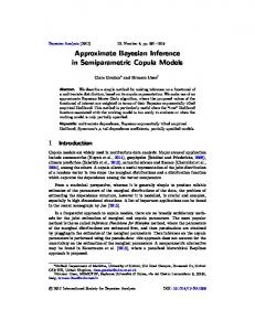
Table 1: Coefficients in the outcome Y-model (6) as estimated using the Bayesian DPM Smodel, where posterior medians and 95% credible intervals are shown; and the frequentist copula S-model of BG, where MLE and SEs are shown. To further understand the improved precision in the Y-model, it is useful to look at the results of the DPM S-model. As shown in the scatter plot of a representative posterior draw of the principal strata (Di (0), Di (1)) in Figure 1(a), there are three predominant clusters: the largest cluster (45% of all units) in the upper right corner, a second largest cluster (30%) in the right middle, and a third (25%) in the lower left corner. Interestingly, these latent clusters have some analogy to the principal strata in the standard binary PS classification (Angrist et al., 1996), but with slight different interpretation since D(0) is placebo compliance and D(1) is drug compliance. Here, the cluster in the upper right corner comprises the full compliers, i.e., units who take the amount prescribed by the protocol, both under treatment and under control. The cluster in the lower left corner includes the never-takers, units who never take what they are assigned to take, neither under treatment, nor under control. Their noncompliance to the protocol is most likely due to behavioral reasons rather than to reasons related to possible sideeffects of the active treatment. Units in the right middle cluster (with D(1) < D(0) < 1) are the most difficult to classify with an analogue in the binary case; we will call them partial compliers. They are units who are generally willing to comply to the protocol if they have no 18
(a)
(b)
Figure 1: (a) A single posterior imputation for (D(0), D(1)) based on the DPM S-model. The green and red dots correspond to units in control and treatment groups, respectively. (b) Median PCE over the entire (D(0), D(1)) space. side effects (i.e., under control), but probably experience negative side-effects under treatment and thus do not take the prescribed amount of the drug. The same cluster structure was consistently observed in all the MCMC chains, and the majority of imputed Dimis maintained a single cluster membership. Thus, for the LRC-CPPT data, there was strong evidence of relevant latent structure recovery, and this information was used to inform Dimis locally on the basis of cluster membership. The reduced variability in estimating the unobserved Dimis lead to more precise estimates of the Y-model. The DPM did not assume side-effect monotonicity, but appears to support the assumption. Figure 1(b) shows the posterior medians of all the PCEs over the entire (D(0), D(1)) space. The PCE surface is smoothly increasing as the compliance increases in both assignment arms, suggesting better compliance behavior is associated to larger overall reduction in cholesterol level. Comparison with the results of JR and BG is made on the estimated PCE at four selected
19
S = (d0 , d1 )
DPM
Parametric (JR)
Copula (BG)
(1, 1)
45
(38, 52)
50
(39, 59)
51
(0.89, 0.70)
29
(25, 34)
24
(17, 30)
30
(1, 0)
0
-
-13
(-42, 27)
0
(0, 0)
0
-
5
(-6, 16)
0
Table 2: Estimated PCE for selected principal stratum (D0 , D1 ) using the DPM approach, the fully parametric approach of JR, and the copula approach of BG. principal stratum S = (d0 , d1 ), including the stratum of “median complier” under both assignments, S = (0.89, 0.70). The comparison is displayed in Table 2, which includes the posterior medians and 95% credible intervals for the PCEs under the DPM approach, and the corresponding estimates from the fully Bayesian parametric approach of JR and the copula approach of BG. The discrepancy between the entries of the final two rows of Table 2 is a result of the mean specifications (6). The results are comparable across methods, while the DPM approach provides tighter estimate intervals than the fully parametric approach, which again highlights the improved precision that results from the clustering structure imposed by the DP. Interval estimates were not provided by BG. In addition, the DPM S-model reveals clusters of the latent principal strata that have natural interpretation as in the binary PS case.
4 4.1
Application to the Swedish National March Cohort Data and Models
This section examines the effect of physical activity (PA) on cardiovascular disease (CVD) as it relates to body mass index (BMI) using the observational Swedish National March Cohort (NMC). The NMC was established in year 1997, when 300,000 Swedes participated in a national fund-raising event organized by the Swedish Cancer Society. Every participant was 20
asked to fill in a questionnaire that included items on known or suspected risk factors for cancer and CVD. Questionnaire data were obtained on over 43,880 individuals. Using the Swedish patient registry, these individuals were followed for the period from year 1997 to 2004, and each CVD event was recorded. Further details on the NMC can be found in Lagerros (2006). The question of scientific interest here is the extent of a causal effect of PA on CVD risk mediated or not mediated through BMI. The principal strata with respect to the intermediate variable BMI is the joint potential values of BMI for an individual under high and low exercise regimes. The PCEs in the principal strata consisting of individuals whose BMI remains the same regardless of exercise can be interpreted as the (principal strata) direct effect (PSDE) of exercise on CVD not mediated through BMI. Similarly, we can define the (principal strata) mediated effect (PSME) as the PCEs in the principal strata of individuals whose BMI would change due to exercise. Sj¨olander et al. (2008), hereafter SJ, analyzed the NMC data using PS, where each subject is classified as either a “low-level exerciser” (T = 0) or a “high-level exerciser” (T = 1) based on self-reported history of PA; obese (D = 1) or not obese (D = 0) based on baseline BMI in year 1997 dichotomized at cutoff point 30; and “with disease” (Y = 1) or “without disease” (Y = 0) based on if the subject had at least one CVD event recorded during follow-up. Age is a strong confounder in this setting, and is the sole covariate reported in SJ. In what follows, in order to compare with the SJ analysis, we also assume that T is ignorable given age. The PSDEs are the main causal estimands in SJ, and they found evidence for beneficial PSDEs. In the current analysis, we follow the definition of T and Y in SJ, but analyze D (BMI) in its original continuous scale and let Xi = (Xi1 , Xi2 ) be the centered age and square of age. In addition, we will investigate both PSDEs and PSMEs. Of the participants, 38,349 were “high-exercisers” and 2,956 were “low-exercisers”. The former included 2,262 cases of CVD, while the latter included 172. The distribution of age is similar in both arms, with the T = 1 arm being slightly older on average. The median age is
21
49.3 years in T = 0 arm and 52.2 in T = 1. The distribution of BMI is right skewed in both arms, with a heavier tail in the low-exercise arm, as seen in Figure 2 top left panel. The median BMI in the T = 0 and T = 1 arms are 24.8 and 24.0, respectively. A quantile-quantile plot of BMI in the two arms (Figure 2 top right panel) suggests the high-exercisers have lower BMI than the low-exercisers on average. There appears to be a strong positive correlation between CVD incidence and BMI (Figure 2 bottom right panel), with a larger variance of CVD in the low-exerciser arm. Likelihood ratio tests on the observed marginal distribution of Y (0) and Y (1) further suggest that both age and BMI are significant predictors of CVD risk in both arms. Based on the above exploratory data analysis, we have experimented various specifications of the Y-model. Among those, the following form leads to the most stable model fitting and natural interpretation, logit{Pr(Yi (0) = 1|Si , Xi )} = β0Y + β1Y Xi1 + β2Y Di (0) logit{Pr(Yi (1) = 1|Si , Xi )} = β0Y + β1Y Xi1 + β2Y Di (0) + β3Y Di (1) + β4Y
Di (0) . (7) Di (1)
Here, the Y (0) model specifies the regression of CVD on BMI when an individual does not exercise. In the Y (1) model, the term β2Y Di (0) + β3Y Di (1) can be re-written as (β2Y + β3Y )Di (1) + β2Y (Di (0) − Di (1)). Thus, β2Y + β3Y can be interpreted as the baseline effect of BMI on CVD when an individual exercises, while β2Y and β4Y represent the additional linear and nonlinear (ratio) effect of the change in BMI due to exercise on CVD, respectively. The Y (1) specification is a key modeling assumption because it allows the relationship to be induced between Di (0) and Di (1) even though they are not jointly observed. Sharing β0 , β1 and β2 across the Y (0) and Y (1) specification leads to parsimonious models, which is important for stable model fitting here. The prior distribution for β Y = (β0Y , β1Y , β2Y , β3Y , β4Y ) is set to be a diffused normal Pr(β Y ) = N(0, 52 I5 ). Scatterplot of average BMI versus age shows a positive and curvilinear relationship between age and BMI (Figure 2 bottom left panel). Likelihood ratio tests on the observed marginal 22
BMI Frequency
QQ−plot of BMI in T=0 versus T=1 ●
0.12
●
45
●
●
●
●
●
●
●
●
●
●
●
●
●
●
●
●
●
●
●
●
●
●
●
●
●
●
● ●
●
●
●
● ●
●
● ●
●
●
●
●
●
●
●
●
●
●
35
●
● ● ● ●
● ●
●
●
●
●
●
●
●
●
●
●
●
●
●
●
●
●
●
●
●
●
● ●
●
●
●
●
●
● ● ●
●
●
●
●
●
●
●
● ●
●
●
●
● ●
●
● ●
● ●
●
●
● ● ●
● ●
●
●
●
●
● ●
● ● ●
●
●
●
●
●
●
●
●
●
●
● ●
●
●
●
●
●
●
●
●
●
●
●
●
●
●
● ●
●
●
●
● ●●
● ●
● ●
●●
●
●
●
●
●
●
●
●
●
● ●
●
●
●
●
●
● ● ●
●
●
●
●
●
●
● ●
●
●
● ●
●
●
●
●
●
●
●
●
●
●
●
● ●
● ●
●
●
● ●
●
●
●
●
●
●
●
●
●
● ●
●
● ● ● ● ●
● ● ●●
●
●
●
●
● ●
●
●
●
●
●
●
●
●
● ● ● ●
●
●
● ●●
●●
●
●
●
●
●
●
● ●
●
●
●
●
● ● ●
●
●
●
●
●
●
●
● ●
●
●
● ● ●● ●●
●
●
●
●
● ●
●
●
●
●
●
●
●
● ● ● ● ●
●
●
●
●
●
●
●
● ●●●
●
●
●
●
●
●
●
●
●
● ● ● ●
●
●
●
●
●
●
● ●●
●●
● ● ● ●
● ●
●
●
●
●
●
● ●●
●
●●
● ●
●
●
●
●
●
●
●● ● ●
●
● ●
● ●●
●
● ● ●● ● ●
●
●
●
● ● ●
●
●
●
●●
● ●
● ●
●
● ● ●
● ●
●●●
●
●
● ● ●
●
● ●
● ●
●
● ● ● ● ●
●
●
●
● ●
●
●
● ●●
●
● ● ●
●
●
●
●
● ● ●●
● ● ●
●
●
●
●
●
●
●
●
●
●
●
●
●
●
●
●
●
● ●
● ●
●
●
●●
● ● ●
●
● ●
●
● ●
●
● ●
●
●
●
●
● ●
●
●
●
●
● ●● ●
●
● ●
●
●
● ● ●
●
●
● ●●●
●
●
●
●
● ●
●
●
●
● ●
●
●
●
●
● ● ● ● ● ●
●
●
●
●
● ●
●
●
●
●
●
●
●
● ●
●
●
●
● ●● ● ●
●
● ●
●
●
●
●●
●
●
● ● ● ●
●
●
●●
● ●
●
●● ●
● ●
●
●
●●
●
●
●
●
● ●
●
● ●
● ●
● ● ●
●
●●
●
●
● ●
● ●
●
●
●
●
●
● ●
●●
●
●
● ● ●
●●
● ●●
●
● ● ●
●
●
●
●
●● ●
●
●
●
●
●
●
●
● ●●
●
●
● ●
● ●
●
●
●
●
●
●
●
●
● ● ● ● ●
●
● ●
●
●
●
●
●
25
T=0
0.06
T==1 T==0
●
● ●
● ●
●
●
● ●
●
●
●
●
●●
●
●
●● ●
●
● ●
● ●
● ●
●
● ●
●
● ● ●
●
●
● ● ●
●
● ● ●
●●
●
●
●
●
●●
●
●
●
● ●
●
●
●
●
●
● ●
●
● ●
●
● ● ●
●
●
●
● ● ● ●
●
● ● ●
●
●
● ● ● ● ● ●
●
●
●● ●
●
● ●
●
●
●
●
● ●
●
● ● ● ● ●
● ●
●
●● ● ●
●
●●
●
●●
●
●
● ●
●
●
● ●●
●
●
●
●
●
● ●
●
●
●
● ●
●
● ●
●
●●
● ●
●
● ●
● ●●
●
●
● ● ●
●
●●
● ●
●
● ●
●
●
●
●
●
● ●
●
●
●
● ●
●
●
● ●
● ●
● ● ● ● ● ● ●
●●
●
●
● ● ●
●
●● ● ●
●
●● ●
●
●
●
● ●●
● ●
● ●
●
●
●
●●
● ● ●
● ●
●
●
●
● ●
● ●
●
●●●
● ●
●
●
●● ● ● ●
●
●
●
●
●
● ●
●
●
● ●
● ● ●
●
●
●
●
●● ● ●
●
●
●
● ● ● ●
●
●●
● ●
● ●
●
● ● ● ●
●● ●
● ●
●
●
●
●
●
●●● ●
● ●
● ● ● ●
●
●
●● ●
●
●
●
●
●
●
●
●
●
●
● ●
●● ●
●●
● ● ● ●
●
● ●●
●
●● ●
●● ●
●
●
●
●
●
● ● ● ●
●
●
●
● ●
●
●
●
●
●
●
●
●
● ●
●
●
● ● ●
●
●●
●●
●
●
● ● ● ●
●
● ●
●
● ●
●
●
● ●
● ●
●
●
●
● ●● ●
●
●
● ●
●
● ●
●
●●
●
● ● ●
●
●
●
● ●● ●
●
●
●●
●
● ● ● ●
●
●
● ●
●
●●
●
●
● ●
● ●
●
●
●
●
● ●
●●
●
● ● ●
●● ●
●
●
●
● ● ● ●
●
●●
●●
●
●
● ●
● ● ●
● ●
●
●●●
●
● ●
●
●
●
●
●
●
●
●● ● ● ●
●
●
●
●
● ● ●
●
●
●
●
● ● ●
●
●● ● ●
●
●
●
●
● ●
● ●
● ●●
● ●
●● ●
●
●
● ●
●
●● ● ●
●
●
●
●
●
● ●
●
● ●
●
●
●
●●
●
● ●
●
●
●
● ●●
●
●
● ●
● ● ● ●●
●
● ●
●
● ●
●
●●
●
●
●
● ●
● ●
●
● ●
●
● ●
●
●
●
●
● ● ●●
● ● ●
●
●
●
● ●
●
● ●
●
● ●
●● ●●
●
●
●
●
●
●
● ●●
● ●
●
●
● ●
●
●● ● ●
●
●
●
●
●
●
●
● ●
●
●
● ●● ●
● ●● ● ●
●
●
●
● ● ●
●● ● ● ●
●
●
●
●
●
●
●
●
●
●
● ● ●
●
●
●
●
● ●
● ● ● ●
●
● ●
●
●
●
●
● ●● ●●
● ●
●
●
● ● ●
●●
● ●
●●
●
● ●
●
●
●
●
●
●
● ●
●
●
●●●
●● ● ●
●
● ●
●
● ●●
●
●
● ● ● ●
●●●
●
●
● ● ●
●
●
●
●
●
● ●
●
●
●
●
●
● ●
●● ●
●●
●●
●
● ●●
●
●
●
● ● ● ● ●
●
●
● ● ● ●
● ●
●●
●●●●●
● ●●
●
● ● ●
●
●
●
● ●
●
●
●
●
●
●
● ●
●
●
●
●
●
●
●
● ●
●
●
●● ● ●
● ●●
● ●● ●
●●
●
● ●
● ●
●● ●
●
●
●
●
●
● ●
●
●●
●
● ●
● ●
●
●
●
● ● ●
●
●
●
● ●
● ●● ●
●
●
● ●● ● ●
●
●
● ●
● ●
● ●
●
●
● ●
●
●
●
●
● ●
●
●
● ● ●
●●
● ● ●
●
● ●
●
●● ● ● ● ● ● ●
●
●
●
●
●
● ● ● ●
● ● ●
●
●
●
●
● ● ●
● ●
●
●
●
● ●
●
●
●
●
● ●● ●
●
● ●
● ●
●
●
●
● ●
● ● ●
●
● ● ●●
●
●
●
●
●
●
●
●
● ●
●
●
●
● ●
●
●
●
●
●
●
● ●
●
●
●
●
●
● ●
●
●
●
●
●
●
●
●
●
●
●
● ● ●
● ●●
●
●
●
●
●●
●
●
●
●
●
●
●
● ●
●
●
●
●
●
●
●
●
●
● ● ●
●
●
● ●
●
● ●●
●
●
●
● ●
●
●
● ● ●
●
●
●
●
●
● ●
●
●
●
●
●
●
●
●
● ●
●
●
●
●
●
●
●
●
●
● ●
●
●
●
● ●
●
●
●
●
●
●
●
●
●
●
●
●
●
0.00
●
●
● ●
●
●
●
●
●
●
●
●
●
●
●
●
●
15
●
●
●
●
●
●
●
●
●
●
15
19
23
27
31
35
39
15
20
25
30
35
40
45
24
● ● ●
●
●
● ● ● ● ●● ●● ● ● ● ● ● ●
●
● ● ●●●●
● ●
T==0 T==1
●
20
30
40
50
60
70
●
Age 2.5% quantile
●
0.12
26
● ●● ●
●
●
● ●
T==0 T==1
●
● ● ● ●● ● ● ●● ● ● ●● ● ●● ● ● ● ●● ●● ● ●● ● ● ●
●
0.06
●
BMI vs CVD
0.00
●
● ●●
% CVD in BMI 2.5% quantile bins
Age vs BMI
22
Averge BMI in Age 2.5% quantile bins
T=1
● ●
●
●
20
22
24
26
28
30
BMI 2.5% quantile
Figure 2: Top left: frequency of BMI in T = 0, 1 arms. Top right: quantile-quantile plot of BMI in T = 0 versus T = 1 arms. Bottom left: scatter plot of age versus BMI in T = 0, 1 arms. Bottom right: scatter plot of BMI versus CVD incidence in T = 0, 1 arms. distribution of Ds suggest that both age and square of age are significant predictors of BMI in both arms. Thus we assume the following DPM S-model, ∞ D D X η0h + Xi1 β01 + Xi2 β02 , Σh 1A , Pr((Di (0), Di (1))|Xi , β D ) = w h ch N D D η1h + Xi1 β11 + Xi2 β12 h=1
(8)
with A = {(Di (0), Di (1)) : 0 < Di (0), Di (1) < 100}. Specifications for the DP are G0 = N(25I2 , Σ0 )IW(2, 32 I2 ), with σ02 = σ12 = 52 and ρ01 = 0.75, and Pr(α) = Ga(1, 1). The prior distribution for β D is a diffused normal Pr(β D ) = N(0, 102 I4 ). Similarly to the partial compliance application, the posterior distribution of the parameters in the complete data model 23
can be obtained via a Gibbs sampler with data augmentation, which is thus omitted, but is available from the authors upon request.
4.2
Results
The Y-model (7) and DPM S-model (8) are jointly fitted to the NMC data. Similarly as before, five parallel MCMC chains of 205,000 iterations with different starting values were run, with the first 5,000 as burn-in. Mixing of the chains was determined to be adequate and all chains lead to similar posterior summary statistics. Sensitivity of results to alternative hyperparameter specifications for α within the Gamma prior distributions is small and the approximation truncation level H = 10 appears to be adequate for DP approximation in this analysis. Table 3 provides posterior medians and 95% credible intervals for the coefficients. Estimates of β1Y and β2Y suggest that both age and baseline BMI without exercise are positively associate with CVD incidence, while β4Y suggests a sizable reduction in CVD associated with a reduction in BMI due to PA. A representative posterior draw of principal strata (Di (0), Di (1)) along with the DPM configuration from the S-model (8) is displayed in Figure 3(a). There are two predominant clusters that are consistently found throughout all analyses: Component 1 in the middle of the 45o line that consists of around 80% individuals whose BMI is stable regardless of PA; and component 2 above the 45o line that consists of around 15% individuals whose BMI decreases with PA. The precise configuration of remaining components varies in different MCMC chains, but still consistently suggest that the remaining individuals are people who have a even larger reduction in BMI as a result of PA. Figure 3(b) shows posterior medians and 95% credible intervals for PCEs over the plausible range of D(0) and D(1) for individuals who are 60 years old. The PCE surface increases smoothly with both D(0) and D(1), suggesting that the causal effect of exercise in reducing the probability of developing CVD increases as one’s BMI increases. Table 4 provides PCEs 24
coefficient
median
95% cred. ints.
β0Y
-3.48
(-3.65, -3.31)
β1Y
0.10
(0.09, 0.11)
β2Y
0.04
(0.01, 0.08)
β3Y
0.01
(-0.04, 0.04)
β4Y
-0.26
(-0.42, -0.10)
D β01
0.23
(0.21, 0.24)
D β11
0.19
(0.18, 0.20)
D × 102 β02
-0.17
(-0.19, -0.15)
D × 102 β12
-0.15
(-0.16, -0.14)
Table 3: Posterior medians and 95% credible intervals for the coefficients in the Y-model and S-model. for principal strata Si = (d0 , d1 ) that are of scientific interest. BMI values of 18.5, 25, 30, 35 are the standard cutoff points of underweight, overweight, class I obese and class II obese, respectively. Since there are very few individuals with BMI below 18.5, we present the PCEs with BMI being 20 instead. PSDEs are the PCEs on the 45o line. We can see that the PSDEs increase as age and BMI increase. For example, for a person whose BMI is 20 no matter whether he or she exercises, the reduction in CVD risk due to exercise is 0.53% and 1.33% when he or she is 50 and 60 years old, respectively, and the reduction increases to 0.77% and 1.87% respectively if his BMI is always 30. This means that even if exercise does not reduce the BMI, it does reduce the risk of CVD, and the benefit is bigger for older and heavier population. Our results also suggests there is a even bigger PSME of exercise on CVD mediated through BMI. For example, for a person whose BMI reduces from 30 to 25 as a result of exercise, the reduction in CVD risk is 0.92% and 2.23% when he or she is 50 and 60 years old, respectively; and the corresponding reduction is 1.09% and 2.57% respectively for a person whose BMI reduces from 35 to 30 due to exercise. 25
(a)
(b)
Figure 3: (a) A representative posterior draw of principal strata Si under the DPM S-model. Each component is labeled with a number and a light dot representing its mass contribution. The solid line is the 45o line. (b) Median surface and point-wise 95% credible intervals for the PCE, over the relevant space of (D(0), D(1)) for individuals 10 years above the median age (60 years old). The green surface is the reference surface of PCE = 0. The PSDE results here match the findings in SJ. However, analysis of PCE based on continuous BMI offers a more refined picture of the causal mechanism among PA, BMI and CVD risk than that based on dichotomized BMI. In addition, continuous analysis relies less on some standard but untestable identifying assumptions. Specifically, we did not impose the monotonicity assumption (i.e., Di (0) > Di (1)) as in SJ. Monotonicity is a key identifying assumption in the case of binary D. Even if approximately 18% of the posterior draws of (Di (0), Di (1)) do not adhere to monotonicity when it was not enforced (Figure 3(a)), these draws are relatively close to the 45o line. In fact, the PCE surface estimate for the NMC data are rather robust to deviations from this assumption.
26
Age = 50
Age = 60
S = (d0 , d1 )
median
95% cred. ints.
median
95% cred. ints.
(20, 20)
0.53
(0.01, 1.18)
1.33
(0.03, 2.93)
(25, 25)
0.64
(0.23, 1.11)
1.58
(0.57, 2.72)
(30, 30)
0.77
(-0.01, 1.64)
1.87
(-0.02, 3.91)
(35, 35)
0.94
(-0.64, 2.81)
2.21
(-1.53, 6.48)
(25, 20)
0.79
(0.09, 1.48)
1.95
(0.23, 3.65)
(30, 25)
0.92
(0.34, 1.60)
2.23
(0.83, 3.82)
(35, 30)
1.09
(0.08, 2.45)
2.57
(0.20, 5.61)
Table 4: Posterior medians and 95% credible intervals for the percent PCE, E(Y (0)−Y (1)|S = (d0 , d1 )) × 100, for selected principal strata S at age of 50 and 60 years.
5
Discussion
We have proposed a Bayesian semiparametric approach to conduct causal inference in the presence of continuous intermediate variables using the PS framework, where causal estimands are defined on latent subgroups of units, namely the principal strata. Even though never jointly observed, modelling the joint distribution of the two potential intermediate outcomes is critical for PS inference. The key element in our proposal is to model the principal strata by the nonparametric DPM model, which has proved to offer a new approach to causal inference with intermediate variables that has advantages in both inference and interpretability. Specifically, it allowed us to a) overcome the limits of the dichotomization approach, b) exploit the clustering properties of DPMs to explore and interpret the latent structure of the data, c) easily quantify posterior uncertainty on PCEs, without relying on asymptotic approximations. We have illustrated our approach using the randomized LRC-CPPT data, obtaining comparable point estimates but more precise interval estimates than those from existing approaches. We also applied our proposal to the more challenging observational NMC study, and obtained 27
a refined and scientifically sound picture of the causal mechanism between PA, BMI and CVD risk. The ignorability assumption has been assumed throughout the paper. Ignorability usually holds by design in randomized experiments, as the LRC-CPPT trial, but may be more questionable in observational studies. For example, age is the only covariate used in the analysis of NMC data, but there can be many remaining possible confounders, such as sex, genetic profile, etc. Sensitivity to deviations from the ignorability assumption in the PS framework has been explored in Schwartz et al. (2010), but only in the case of binary D. A systematic investigation for such sensitivity in the case of continuous intermediate variable will be helpful. Directions for future research include also extensions of our model, allowing to relax some of the assumptions in the Y-model by, e.g., specifying a DPM also for the conditional distribution of the potential outcomes. Our analysis has shown how crucial the specification of the model for the potential primary outcomes is; therefore, future efforts will include the development of specific tools for assessing model fit, such as posterior predictive checks (Gelman et al., 1996).
Appendix The Gibbs sampler for the partial compliance application. To implement the semiparametric analysis for the LRC-CPPT data, the general Gibbs sampler approach of Section 2.3 is applied to the model specification of Section 3. Unless specified otherwise, parameters reflect the current state of the Gibbs sampler. First initialize the Gibbs sampler by drawing parameter values from their prior distributions. Then, iterate the following steps, 1. Update Dimis for all units as follows, (a) For each i such that Tiobs = 1, draw Dimis , that is, Di (0) from N (v(m1 /v1 + m2 /v2 ), v) 1[0,1] ,
28
� 2 Y Y obs 2 where v = (1/v1 +1/v2 )−1 , v1 = ΣZi ,11 −ΣZi ,12 Σ−1 , Zi ,22 ΣZi ,21 , v2 = σ1 / β1 + β3 Di � obs obs −β0Y −β2Y Diobs )/ β1Y + β3Y Diobs . m1 = η0Zi +ΣZi ,12 Σ−1 Zi ,22 (Di −η1Zi ) and m2 = (Yi (b) For each i such that Tiobs = 0, draw Dimis , that is, Di (1) from � obs N η1Zi + ΣZi ,21 Σ−1 − η0Zi ), ΣZi ,22 − ΣZi ,21 Σ−1 Zi ,11 (Di Zi ,11 ΣZi ,12 1[0,1] . 2. For each i, update the cluster membership Zi using a multinomial distribution with wh ch N ((Di (0), Di (1))0 |(η1h , η0h )0 , Σh ) 1[0,1] Pr(Zi = h|−) = PH , 0 0 k=1 wk ck N ((Di (0), Di (1)) |(η1k , η0k ) , Σk ) 1[0,1] where ch is the normalization constant for the truncated normal. 3. Update wh ’s as Step 3 in Section 2.3. 4. Update α(t+1) from the tth iteration using an independence Metropolis proposal step based on the prior distribution of α. First, sample α∗ from Ga(1, 1). Then set α(t+1) = α(t) , but reassign α(t+1) = α∗ with probability � P P QH−1 ∗ i:Zi >h 1 i:Zi =h 1, α + h=1 Be 1 + �. P P QH−1 (t) + h=1 Be 1 + i:Zi =h 1, α i:Zi >h 1 5. Draw (η1h , η0h )0 from ! N
V
X
(.5, .5)0 /.252 +
0 Σ−1 ,V h (Di (0), Di (1))
! 1[0,1] ,
i:Zi =h
where V = I2 /.252 +
P
−1 i:Zi =h Σh
�−1
, or from the prior N((.5, .5)0 , .252 I2 ) if there are
no units having Zi = h. 6. draw Σh from
X IW 2 + 1, i:Zi =h
I2 +
X i:Zi =h
Di (1) − η1Zi Di (0) − η0Zi
29
Di (1) − η1Zi Di (0) − η0Zi
0 .
7. Finally, update the parameters in the Y -model as follows: (a) Let D(t) = (D1 (t), ..., Dn (t))0 , for t = 0, 1; and define Y (t) analogously. Also let D(0)D(1) = (D1 (0)D1 (1), ..., Dn (0)Dn (1), and 12n = (1, ..., 1)02n . Draw (β0Y , β1Y ) ˜ 0Φ ˜ + I2 /s2 )−1 , M = V (X ˜ 0Φ ˜X ˜ Y˜ + (µ0 , µ1 )0 /s2 ), from N(M , V ), where V = (X ˜ = [12n , (D(0)0 , D(1)0 )0 ], Y˜ = [Y (0)0 , (Y (1)−β Y D(1)−β Y D(0)D(1))0 ]0 , and Φ ˜= X 3 2 diag(In /σ02 , In /σ12 ); and (µ0 , µ1 ) and s2 are the specifications in the prior Pr(β Y |µ, s2 I4 ); (b) Let D1 (t) be the vector of potential outcomes Di (t) for units assigned to treatment group, and define Y1 (t) analogously. Draw (β2Y , β3Y ) from � � � � (D1 (1), D1 (0)D1 (1))0 (Y1 (1) − β0Y − D1 (0)β1Y ) (µ2 , µ3 )0 ,V , + N V σ02 s2 �−1 � 0 where V = (D1 (1),D1 (0)D1 (1))σ2(D1 (1),D1 (0)D1 (1)) + sI22 , and (µ2 , µ3 ) and s2 are the 0
Y
specifications in the prior Pr(β |µ, s2 I4 ). (t+1)
(c) Update λ0
(t+1)
and λ1
using an independence Metropolis proposal step based
on the chosen priors. First, sample λ∗0 from N(3, 1) and λ∗1 from N(0, 1.52 ). Then, set (t+1)
λ0
(t)
(t+1)
= λ0 , but reassign λ0 = λ∗0 with probability Qn obs ∗ obs (t) i=1 N(Yi |ηZi , exp(λ0 + 1Tiobs =1 Di λ1 )) . Qn (t) obs obs (t) i=1 N(Yi |ηZi , exp(λ0 + 1Tiobs =1 Di λ1 ))
Then update λ1 in a similar fashion with probability. Q (t+1) obs + Diobs λ∗1 )) i:Tiobs =1 N(Yi |ηZi , exp(λ0 . Q (t+1) obs (t) obs )) λ |η , exp(λ + D N(Y obs Z 1 0 i i i i:T =1 i
References JD Angrist, GW Imbens, and DB Rubin. Identification of causal effects using instrumental variables. Journal of the American Statistical Association, 91(434):444–455, 1996. F Bartolucci and L Grilli. Modeling partial compliance through copulas in the principal stratification framework. Journal of the American Statistical Association, under revision, 2010. 30
B Efron and D Feldman. Compliance as an explanatory variable in clinical trials. Journal of the American Statistical Association, 86:9–17, 1991. MD Escobar and M West. Bayesian density estimation and inference using mixtures. Journal of the American Statistical Association, 90(430):577–588, 1995. TS Ferguson. Prior distributions on spaces of probability measures. Annals of Statistics, 2: 615–29, 1974. CE Frangakis and DB Rubin. Principal stratification in causal inference. Biometrics, 58(1): 21–29, 2002. AE Gelman, X-L Meng, and HS Stern. Posterior predictive assessment of model fitness via realized discrepancies (with discussion). Statistica Sinica, 6:733–807, 1996. W Imbens and DB Rubin. Bayesian inference for causal effects in randomized experiments with noncompliance. The Annals of Statistics, 25(1):305–327, 1997. H Ishwaran and LF James. Gibbs sampling methods for stick breaking priors. Journal of the American Statistical Association, 96(453):161–173, 2001. H Jin and DB Rubin. Principal stratification for causal inference with extended partial compliance. Journal of the American Statistical Association, 103:101–111, 2008. H Jin and DB Rubin. Public schools versus private schools: Causal inference with partial compliance. Journal of Educational and Behavioral Statistics, 34(1):24–45, 2009. YT Lagerros. Physical activity from the epidemiological perspectivemeasurement issues and health effects. PhD thesis, Department of Medical Epidemiology and Biostatistics, Karolinska Institutet, Stockholm, Sweden., 2006. A Mattei and F Mealli. Application of the prinicipal stratification approach to the faenza randomized experiment on breast self-examination. Biometrics, 63(2):437–46, 2007. 31
P M¨uller and FA Quintana. Nonparametric bayesian data analysis. Statistical Science, 19: 95–110, 2004. PR Rosenbaum. The consquences of adjustment for a concomitant variable that has been affected by the treatment. Journal of the Royal Statistical Society: Series B, 147(5):656– 666, 1984. PR Rosenbaum and DB Rubin. The central role of the propensity score in observational studies for causal effects. Journal of the Royal Statistical Society: Series B, 70(1):41–55, 1983. DB Rubin. Estimating causal effects of treatments in randomized and nonrandomized studies. Journal of Educational Psychology, 66(1):688–701, 1974. DB Rubin. Bayesian inference for causal effects: The role of randomization. The Annals of Statistics, 6(1):34–58, 1978. DB Rubin. Comment on ‘Randomization analysis of experimental data: The fisher randomization test’ by D. Basu. Journal of the American Statistical Association, 75:591–593, 1980. DB Rubin. Comment on ‘Neyman (1923) and causal inference in experiments and observational studies’. Statistical Science, 5:472–480, 1990. SL Schwartz, F Li, and JP Reiter. Sensitivity analysis for unmeasured confounding in principal stratification. Technical report, Department of Statistical Science, Duke University, 2010. J Sethurman. A constructive definition of dirichlet priors. Statistica Sinica, 4:639–650, 1994. A Sj¨olander, K Humphreys, S Vansteelandt, R Bellocco, and J Palmgren. Sensitivity analysis for principal stratum direct effects, with an application to a study of physical activity and coronary heart disease. Biometrics, 65(2):514–520, 2008. MA Tanner and WH Wong. The calculation of posterior distributions by data augmentation. Journal of the American Statistical Association, 82(398):528–540, 1987. 32