The domains calculated by the CVD functionality should be complete (all valid ..... crossed by any long edge, we check for each value v in a domain Di whether it ...
A BDD-Based Polytime Algorithm for Cost-Bounded Interactive Configuration Tarik Hadzic and Henrik Reif Andersen Computational Logic and Algorithms Group IT University of Copenhagen, Denmark {tarik,hra}@itu.dk
Abstract Interactive configurators are decision support systems assisting users in selecting values for parameters that respect given constraints. The underlying knowledge can be conveniently formulated as a Constraint Satisfaction Problem where the constraints are propositional formulas. The problem of interactive configuration was originally inspired by the product configuration problem with the emergence of the masscustomization paradigm in product manufacturing, but has also been applied to other tasks requiring user interaction, such as specifying services or setting up complex equipment. The user-friendly requirements of complete, backtrack-free and real-time interaction makes the problem computationally challenging. Therefore, it is beneficial to compile the configuration constraints into a tractable representation such as Binary Decision Diagrams (BDD) (Bryant 1986) to support efficient user interaction. The compilation deals with the NPhardness such that the online interaction is in polynomial time in the size of the BDD. In this paper we address the problem of extending configurators so that a user can interactively limit configuration choices based on a maximum cost (such as price or weight of a product) of any valid configuration, in a complete, backtrack-free and real-time manner. The current BDD compilation approach is not adequate for this purpose, since adding the total cost information to the constraints description can dramatically increase the size of the compiled BDD. We show how to extend this compilation approach to solve the problem while keeping the polynomial time guarantees.
Introduction Interactive configuration problems are special applications of Constraint Satisfaction Problems (CSP) where a user is assisted in interactively assigning values to variables by a software tool. The key user functionality delivered by this tool is the calculation of valid domains (CVD) for each unassigned variable. Application areas include customizing physical products (such as PC’s and cars) and services (such as airplane tickets and insurances). The domains calculated by the CVD functionality should be complete (all valid configurations should be reachable through user interaction), backtrack-free (a user is never forced to change an earlier choice due to incompleteness in c 2006, American Association for Artificial IntelliCopyright gence (www.aaai.org). All rights reserved.
the logical deductions), and the CVD feedback should be in real-time. The requirement for backtrack-freeness and completeness makes the problem of calculating valid domains NP-hard. Therefore, in order to provide real-time guarantees, current approaches use off-line compilation of the CSP model into a tractable datastructure representing the solution space of all valid configurations (Møller, Andersen, & Hulgaard 2001; Amilhastre, Fargier, & Marquis 2002; Madsen 2003). Although having exponential worst-case size, in the real industrial applications that are using BDDs, the compiled representations can often be kept small (Hadzic et al. 2004; Subbarayan et al. 2004). In this paper we look at the problem of cost-bounded interactive configuration, where every selectable value is assigned a cost. The extended CVD functionality, denoted as max-bounded CVD, should allow a user to limit the maximum cost for any final valid configuration. This problem corresponds closely to an important product-configuration functionality where a user can interactively limit the maximum cost of any configurable specification, such as price or weight of the configured product. We first describe CVD functionality for the standard BDD-based configuration. Then we show that the immediate approach to cost bounded configuration can lead to exponential explosion in the size of the BDD representation. We then construct algorithms that augment the BDD representation to deliver max-bounded CVD with polynomial-time guarantees. Finally, we show that it is not possible to extend polynomial-time guarantees for cost-bounded configuration where domains are restricted by both minimum and maximum bounds. The remainder of the paper is organized as follows. In the next section we formalize the concept of interactive configuration, afterwards we describe the BDD-based configuration approach. The main section describes a solution approach to cost-bounded configuration. Before we conclude we discuss the complexity of some extensions to the cost-bounded approach.
Interactive Configuration The input model describing the knowledge about valid variable assignments is a special kind of a Constraint Satisfaction Problem (CSP) (Dechter 2003): A configuration model C is a triple (X, D, F ) where X is
a set of variables {x0 , . . . , xn−1 }, D = D0 × . . . × Dn−1 is the Cartesian product of their finite domains D0 , . . . , Dn−1 and F = {f0 , ..., fm−1 } is a set of propositional formulae over atomic propositions xi = v, where v ∈ Di , specifying conditions on the values of the variables. Concretely, every domain can be viewed as Di = {0, . . . , |Di | − 1}. An assignment of values v0 , . . . , vn−1 to variables x0 , . . . , xn−1 is denoted as a set of pairs ρ = {(x0 , v0 ), . . . , (xn−1 , vn−1 )}. The domain of the assignment dom(ρ) is the set of variables which are assigned: dom(ρ) = {xi | ∃v ∈ Di .(xi , v) ∈ ρ} and if dom(ρ) = X we refer to ρ as a total assignment. We say that a total assignment ρ is valid if it satisfies all the rules, which is denoted as ρ |= F . A partial assignment ρ, dom(ρ) ⊆ X is valid if there is at least one total assignment ρ0 ⊇ ρ that is valid, ρ0 |= F , i.e. if there is at least one way to successfully complete the existing configuration process. In product configuration, the knowledge about product components and product rules is usually modelled by representing all the choices for a component as values in a variable domain. Then, a valid total assignment ρ completely specifies a configurable product.
User Interaction A configurator assists a user interactively in reaching a valid product specification, i.e. in reaching a valid total assignment. The key operation in this interaction is that of computing, for each unassigned variable xi ∈ X \ dom(ρ), the valid domain Diρ ⊆ Di . The domain is valid if it contains those and only those values with which ρ can be extended to become a total valid assignment ρ0 , i.e. Diρ = {v ∈ Di | ∃ρ0 : ρ0 |= F ∧ ρ ∪ {(xi , v)} ⊆ ρ0 }. The significance of this demand is that it guarantees the user backtrack-free assignments to variables as long as he selects values from valid domains. This reduces cognitive effort during the interaction and increases usability. At each step of the interaction, the configurator reports the valid domains to the user, based on the current partial assignment ρ resulting from his earlier choices. The user then picks an unassigned variable xi ∈ X \ dom(ρ) and selects a value from the calculated valid domain vi ∈ Diρ . The partial assignment is then extended to ρ ∪ {(xi , vi )} and a new interaction step is initiated.
BDD Based Configuration
In (Møller, Andersen, & Hulgaard 2001; Hadzic et al. 2004; Subbarayan et al. 2004) the interactive configuration was delivered by dividing the computational effort into an offline and online phase. First, in the offline phase, the authors compiled a BDD (Bryant 1986) representing the solution space of all valid configurations Sol = {ρ | ρ |= F }. Then, the functionality of calculating valid domains (CVD) was delivered online, by efficient algorithms executing during the interaction with a user. The benefit of this approach is that the BDD needs to be compiled only once, and can be reused for multiple user sessions. An important requirement for online user interaction is the guaranteed real-time experience of the user configurator interaction. Therefore, the algorithms that are executing
in the online phase must be provably efficient in the size of the BDD representation. This is what we call the real-time guarantee. As the CVD functionality is NP-hard, and the online algorithms are polynomial in the size of the generated BDD, there is no hope of providing polynomial size guarantees for the worst-case BDD representation. However, it suffices that the BDD size is small enough for all the configuration instances occurring in practice (Subbarayan et al. 2004).
Compiling the Configuration Model To compile a configuration model into a BDD, each of the finite domain variables xi with domain Di = {0, . . . , |Di | − 1} is encoded by ki = dlog|Di |e Boolean variables xi0 , . . . , xiki −1 , referred to as log encoding variables. Each v ∈ Di , corresponds to a binary encoding v0 . . . vki −1 denoted as v0 . . . vki −1 = enc(v). Also, every combination of bits v0 . . . vki −1 represents some integer v ≤ 2ki − 1, denoted as v = dec(v0 . . . vki −1 ) such that dec(enc(v)) = v. Hence, the atomic proposition xi = v is encoded as a Boolean expression xi0 = v0 ∧ . . . ∧ xiki −1 = vki −1 . In addition, domain constraints are added to forbid those bit assignments v0 . . . vki −1 which do not translate to a value in Di , i.e. where dec(v0 . . . vki −1 ) ≥ |Di |. Assuming the ordering x0 < . . . < xn−1 , a solution space Sol is represented by a Reduced Ordered Binary Decision Diagram B(V, E, Xb , R, var), where V is a set of nodes ranged over by u, including the terminal nodes T0 , T1 . E is the set of edges ranged over by e and Xb = {0, 1, . . . , |Xb |−1} is set of variable indices, labelling every non-terminal node u with var(u) ≤ |Xb | − 1 and labelling the terminal nodes T0 , T1 with index |Xb |. The set of variable indices Xb is constructed by taking the union of the Sn−1 log-encoding variables i=0 {xi0 , . . . , xiki −1 } and ordering them in a natural layered way, i.e. xij11 < xij22 iff i1 < i2 or i1 = i2 and j1 < j2 . Every directed edge e = (u1 , u2 ) has a starting vertex u1 = π1 (e) and ending vertex u2 = π2 (e). R denotes the root node of the BDD.
Standard CVD Algorithms In this section we will briefly revisit how the calculation of valid domains is executed in the standard configuration case. The description is based on the Clab (Jensen online) configuration framework, and a more detailed formalization can be found in (Hadzic, Jensen, & Andersen 2006 online). Before describing the algorithms, we first introduce the appropriate notation. Let xij be the j + 1-st Boolean variable encoding the finite domain variable xi . Then, if xij corresponds to an index k ∈ Xb we define var1 (k) = i and var2 (k) = j to be the appropriate mappings. Now, given the BDD B(V, E, Xb , R, var), Vi denotes the set of all nodes u ∈ V that are labelled with a BDD variable encoding the finite domain variable xi , i.e. Vi = {u ∈ V | var1 (u) = i}. We think of Vi as defining a layer in the BDD. We define Ini to be the set of nodes u ∈ Vi reachable by an edge originating from outside the Vi layer, i.e. Ini = {u ∈
Vi | ∃(u0 , u) ∈ E. var1 (u0 ) < i}. For the root node R, labelled with i0 = var1 (R) we define Ini0 = Vi0 = {R}. Now we will more precisely denote the interaction process in which a user extends the partial assignment by assigning values from valid domains to unassigned variables. We assume that we are in an interaction step where in the previous user assignment, a user fixed a value for a finite domain variable x = v, x ∈ X, extending the old partial assignment ρold to the current assignment ρ = ρold ∪{(xi , v)}. For every variable xi ∈ X, old valid domains are denoted as Diρold , i = 0, . . . , n − 1, and the old BDD B ρold is reduced to a restricted BDD, B ρ (V, E, Xb , R, var). Note that for assigned variables xi ∈ dom(ρold ), Diρold = {ρ(xi )} and the log-encoding variables Xb correspond only to variables X \ dom(ρold ). The CVD functionality is to calculate valid domains Diρ for the remaining unassigned variables xi 6∈ dom(ρ) by extracting values from the newly restricted BDD B ρ (V, E, Xb , R, var). To simplify the following discussion, we will analyze the isolated execution of the CVD algorithm over a given BDD B(V, E, Xb , R, var). The task is to calculate valid domains V Di from the starting domains Di . The user-configurator interaction can be modelled as a sequence of these executions over restricted BDDs B ρ , where the valid domains are Diρ and the starting domains are Diρold . A value v ∈ Di is in V Di if there is a path in B from the root to the terminal T1 consistent with the binary encoding of v. The CVD functionality is implemented by observing two key ideas on when we can conclude if there is such a path. First, this happens if there is a long edge e = (u1 , u2 ) crossing over layer Vi , i.e. var1 (u1 ) < i < var1 (u2 ) such that u2 6= T0 . Then we can include all the values from Di into a valid domain, i.e. V Di = Di . Detecting and copying of all ”skipped” variable domains can be achieved in O(|E| + n) where |E| is the number of edges in the compiled BDD B and n = |X| is the number of finite domain variables. For more details check (Hadzic, Jensen, & Andersen 2006 online). For the remaining variables xi , whose layer Vi is not crossed by any long edge, we check for each value v in a domain Di whether it can be part of the domain V Di . The second key observation is that if v ∈ V Di then there must be u ∈ Vi such that traversing the BDD from u with logencoding of v will lead to a node other than T0 . This is sufficient since from any non-zero node u ∈ V \ {T0 } it is possible to reach the terminal T1 , i.e. possible to satisfy the BDD B. Traversing u ∈ Vi with value j ∈ Di is depicted by the algorithm in Fig. 1. It is important to note that the marking scheme for each j ∈ Di prevents processing the same node more then once. Hence, to calculate V Di it takes at most O(|Vi | · |Di |) steps. Now, the total worst-case running time to implement the classical CVD functionality is Pn−1 Pn−1 O(( i=0 |Vi | · |Di |) + |E| + n) = O( i=0 |Vi | · |Di | + n).
T raverse(u, v) 1: i ← var1 (u) 2: v0 , . . . , vki −1 ← enc(v) 3: repeat 4: if M arked[u] = v return T0 5: M arked[u] ← v 6: s ← var2 (u) 7: if vs = 0 then u ← low(u) 8: else u ← high(u) 9: until var1 (u) 6= i 10: return u Figure 1: For fixed u ∈ V, i = var1 (u), T raverse(u, v) iterates through Vi and returns the node in which the traversal ends up according to the value v. M arked[u] is initialized to −1.
Interactive Maximum Cost Bounded Configuration We now consider an extension of the configuration model where the selection of each choice v ∈ Di is associated with a cost. A cost bounded configuration model Cc is a quadruple (X, D, F, c) where C(X, D, F ) is a standard configuration model and c is a cost function such that civ ∈ Z denotes the integer cost of choice xi = v, xi ∈ X, v ∈ Di . P The cost of assignment ρ is defined as c(ρ) = i ciρ(xi ) . Given the starting domains Di , partial user assignment ρ and a user-designated maximum cost Cmax , the configurator should calculate and display the valid domains involving only those choices that can be extended to a configuration of maximum price Cmax . The cost-bounded valid domains are: Diρ,Cmax = {v ∈ Di | ∃ρ0 .(ρ0 |= F and ρ ∪ {(xi , v)} ⊆ ρ0 and c(ρ0 ) ≤ Cmax )}. In the following subsections we will discuss how to implement this functionality.
Encoding Costs in the BDD To simplify the following discussion we assume that the costs civ are non-negative integers. An immediate approach to deliver max-bounded CVD is to create a new configuration model Cy by introducing a new variable y ∈ Dy to the configuration model C and adding appropriate propositional constraints enforcing for any solution ρ X y= (1) ciρ(xi ) . i
We then generate a new BDD representation B y and let the user manipulate the cost in the standard configuration process. The user can for example specify the exact price of the final product y = v and in return get valid options Di for other unselected components xi . A constraint y ≤ Cmax can be encoded as y = 0 ∨ y = 1 ∨ . . . ∨ y = Cmax . We claim that this approach is inadequate since the size of B y can be exponential in the model encoding Cy even for the practical instances where B is of manageable size. This would make efficient CVD algorithms unusable since they operate over the exponentially large structure.
Let x0 < . . . < xi−1 < y < xi+1 < . . . < xn be a variable ordering where the variable y is in the i-th place (xi = y). Let C Sol (X 0 ) denote the set of all different costs over all valid P combinations of variables in X 0 ⊆ X, i.e. C Sol (X 0 ) = { xi ∈X 0 ciρ(xi ) | ρ ∈ Sol}. Let V y denote the set of vertices in BDD B y . We have the following: Theorem 1. |V y | ≥ max(|C Sol ({x0 , . . . , xi−1 })|, |C Sol ({xi+1 , . . . , xn })|) 1 Proof. It suffices to notice the following: For every cost of a valid partial assignment c(ρ) ∈ C Sol ({x0 , . . . , xi−1 }) there must be at least one node u ∈ Iny . Namely, if there were more costs than nodes then there is a node u0 ∈ Iny for which there are at least two partial assignments ρ1 , ρ2 of different costs c(ρ1 ) 6= c(ρ2 ) such that traversing from R through both ρ1 and ρ2 ends up in u0 . This means that for any valid partial assignment ρ3 traversing from u0 to T1 we have the same total price ρ3 (y)P (from equation (1)) equal to n two different numbers c(ρ1 ) + k=i+1 ckρ3 (xk ) and c(ρ2 ) + Pn k k=i+1 cρ3 (xk ) , which is not possible. With similar reasoning, we conclude that for cost of a valid partial assignment c(ρ) ∈ C Sol ({xi+1 , . . . , xn }) there must be at least one node in Outy = {u2 ∈ V | ∃(u1 , u2 ) ∈ E.(var(u1 ) = i and var(u2 ) > i)} . Hence, |V y | ≥ max(|Iny |, |Outy |) ≥ max(|C Sol ({x0 , . . . , xi−1 })|, |C Sol ({xi+1 , . . . , xn })|) Now, it is easy to construct instances where By explodes while B is small. For example, if all the variables are Boolean except y, and each ci1 = 2i and ci0 = 0, and we have no constraints F = {} (leading to always true BDD), we have |B| = 1 but |B y | > 2bn/2c .
An Extended BDD Compilation Approach The basic idea behind our approach is not to introduce the price variable y into the model, but to process a user restriction c(ρ) ≤ Cmax by additional filtering during online execution of CVD algorithms. By doing this, we do not risk an exponential blow-up of the BDD representation. We can therefore construct the CVD algorithms without sacrificing the processing guarantee. In order to calculate valid domains V Di , we need to be able to determine for a value v ∈ Di with designated cost civ whether it is possible to find an assignment ρ |= F , such that ρ(xi ) = v and c(ρ) ≤ Cmax . In other words, we need to check if there is an assignment ρ = ρ1 ∪ {(xi , v)} ∪ ρ2 such that c(ρ1 ) + civ + c(ρ2 ) ≤ Cmax , dom(ρ1 ) = {x0 , . . . , xi−1 }, dom(ρ2 ) = {xi+1 , . . . , xn−1 }. To illustrate the key idea, assume that a path σ in layer Vi (referred to as i-path σ), is encoding a value v ∈ Di , i.e. σ = {(u1 , u2 ), . . . , (uk−1 , uk )} such that uk = 1
From Theorem 1 we see that unless many values in the domains share identical costs, the BDD B y is likely to explode. In fact, if any of |C Sol ({x0 , . . . , xi−1 })| or |C Sol ({xi+1 , . . . , xn })| is exponentially large, it is guaranteed that |By | will be exponentially large.
R U[u1 ] u1
Vi
u2
uk
D[uk ] T1
Figure 2: An i-path σ = {(u1 , u2 ), . . . , (uk−1 , uk )} encoding the value v ∈ Di . U [u] and D[u] denote the costs of cheapest paths from u to R and T1 respectively. If the cost U [u1 ] + cv (σ) + D[uk ] ≤ Cmax then v is in the valid domain. T raverse(u1 , v) and var1 (uk ) = i + 1. The cost of path σ is c(σ) = civ . Let ρuup1 be the cheapest assignment to variables {x0 , . . . , xi−1 } that when traversed from root R k be the cheapest assignends up in u1 . Also, let ρudown ment to variables {xi+1 , . . . , xn−1 } that traverses from uk and ends up in T1 . Let us denote c(ρuup1 ) as U [u1 ] and k c(ρudown ) as D[uk ]. Now to test whether path σ allows value v to be added to V Di it suffices to check whether U [u1 ] + c(σ) + D[uk ] ≤ Cmax . This is illustrated in Fig. 2. The key idea is to efficiently calculate the values U [u1 ] and D[uk ] for every i-path σ = {(u1 , u2 ), . . . , (uk−1 , uk )}. Note that this requires u1 ∈ Ini and that the last edge (uk−1 , uk ) ∈ E that is crossing out of the layer Vi can be a long edge such that for i2 = var1 (u2 ) it holds i2 > i + 1. Also, a path σ could encode more than one value v ∈ Di since some of the internal edges (uj , uj+1 ) might be skipping variables, allowing for more then one value. The cost of σ encoding the value v is denoted as Pi2 −1 l cmin where clmin is the cheapest value cv (σ) = civ + l=i+1 l l −1 {clj }. Now, for every i-path in Dl , i.e. cmin = minkj=0 σ = {(u1 , u2 ), . . . , (uk−1 , uk )} encoding value v ∈ Di , it holds: U [u1 ] + cv (σ) + D[uk ] ≤ Cmax ⇒ v ∈ Di . Augmented Labelled Graph In order to efficiently compute labels U [u], D[u] we introduce an Augmented Labelled Graph G0 (V 0 , E 0 , w). It is a directed acyclic graph constructed from BDD B(V, E, Xb , R, var) that allows efficient computation of these labels by running the efficient single-source shortest-path algorithms. The key idea is to add augmented edges, e0 = (u1 , u2 ) between any two nodes u1 ∈ Ini , var1 (u2 ) > i when there exists an i-path σ between u1 and u2 encoding a value v ∈ Di . In other words, Ei0 = {(u1 , u2 ) | u1 ∈ Ini and ∃v ∈ n−1 0 Di .u2 = T raverse(u1 , v)} and E 0 = ∪i=0 Ei . Let wmin (u1 , u2 ) denote the cost of the cheapest assignment civ among all v ∈ Di such that u2 = T raverse(u1 , v).
The cost of the entire edge is w(u1 , u2 ) = wmin (u1 , u2 ) + Pi2 −1 i k=i+1 cmin . Actually, w(u1 , u2 ) is equal to the price of the cheapest i-path σ between u1 and u2 . The construction algorithm is shown in Fig. 3. ConstructGraph(B) 1: E 0 ← {},V 0 ← {R} 2: for i = 0 to n − 1 3: for each v ∈ Di 4: for each u1 ∈ Ini 5: u2 ← T raverse(u1 , v) 6: if (u1 , u2 ) 6∈ E 0 then w(u1 , u2 ) ← ∞ 7: E 0 ← E 0 ∪ {(u1 , u2 )}, V 0 ← V 0 ∪ {u2 } 8: i2 ← var1 (u2 ) Pi2 −1 k 9: t ← civ + k=i+1 cmin 10: if w(u1 , u2 ) > t then 11: w(u1 , u2 ) ← t,wmin (u1 , u2 ) ← civ 12: return (V 0 , E 0 , w) Figure 3: Adds augmented edges (u1 , u2 ) to the graph and labels them with the cost of the cheapest path from u1 to u2 . Pn−1 The running time is O( i=0 |Vi | · |Di |) where the marking scheme in T raverse(u1 , v) ensures that for every v ∈ Di at most |Vi | vertices are traversed. The induced graph Pn−1 G0 (V 0 , E 0 ) has at most i=0 |Ini | · |Di | edges, since we add at most |Di | edges for every node u ∈ Ini . Since we do not introduce any new nodes, and possibly delete some internal nodes it holds: |V 0 | ≤ |V |.
Augmented CVD Algorithms In this section we show how to calculate new domains V D0 , . . . , V Dn−1 that also satisfy the maximum cost restriction. The first step is to label the nodes u ∈ V 0 of the augmented graph G0 with U [u], D[u]. It suffices to run two single-source shortest path algorithms, from root R and terminal T1 each. The resulting distances are exactly the values for our U and D labels. The shortest-path algorithms are well described in details in (Cormen et al. 2001). Since G0 is a directed acyclic graph the running time is O(|E 0 |+|V 0 |). Then, in order to calculate valid domains of variables skipped by a long edge, we execute the algorithm in Fig. 4 which calculates for every variable xi ∈ X the cost of the cheapest path skipping over layer Vi . In other words, the algorithm calculates the price of the cheapest path involving an edge (u1 , u2 ) ∈ E 0 such that var1 (u1 ) < i < var1 (u2 ). The price of such minimal cost path is stored in P [i]. Topological sorting takes O(|E 0 | + |V 0 |) time. For every long edge (u, u0 ) we execute line 4, var1 (u0 ) − var1 (u) − 1 times. Hence, if we denote X((u, u0 )) = {var1 (u) + 1, . . . P , var1 (u0 ) − 1}, then the worst-case execution time is O( e∈E 0 |X(e)|) + O(|E 0 | + |V |) = O(|E 0 | · n) = Pn−1 Pn−1 O(( i=0 |Ini | · |Di |) · n) = O(( i=0 |Vi | · |Di |) · n). After calculating cheapest skipping paths, the algorithm in Fig. 5 efficiently extracts valid domains with respect to interactively provided maximum-cost limit Cmax .
CheapestP aths(G0 ) 1: for all i = 0, . . . , n − 1, P [k] ← ∞, 2: for all (u, u0 ) ∈ E 0 in increasing topological order, u0 6= T0 3: for l = var1 (u) + 1 to var1 (u0 ) − 1 4: P [l] ← min{P [l], U [u]+w(u, u0 )+D[u0 ]} Figure 4: For every variable xk the algorithm calculates P [k], the cheapest path in the augmented graph spanning across the Vk , i.e. allowing for any assignment to xk . Obviously, such a path might not exist, in which case P [k] = ∞. CVDRuntime(B, Cmax ) 1: for each i = 0 to n − 1 2: max ← Cmax + cimin − P [i] 3: V Di ← {v ∈ Di | civ < max} 4: for each v ∈ Di \ V Di 5: for each u1 ∈ Ini 6: u2 ← T raverse(u1 , v) 7: if u2 6= T0 and U [u1 ] + w(u1 , u2 )− wmin (u1 , u2 ) + civ + D[u2 ] ≤ Cmax 8: then 9: V Di ← V Di ∪{v}, skip to next v Figure 5: The algorithm extracts valid domains from BDD B, based on maximum cost Cmax . It uses all the auxiliary labels U [u], D[u], P [i], w(u1 , u2 ), wmin (u1 , u2 ) that were precalculated in previous steps. If P [i] − cimin + civ ≤ Cmax then the cheapest path P [i] crossing the layer Vi allows to include the cost of value v ∈ Di instead of the minimal cost cimin . The maximum bound for such civ that can be included is calculated in line 2, and then all the values cheaper then this maximum bound are added to V Di in line 3. Note that if there is no cheapest path then P [i] = ∞ and no values are added. For each i this step executes in O(|Di |) time. For the rest of the values v ∈ Vi \ V Di it is checked whether there is an induced edge (u1 , u2 ) that is compatible with v such that the price of traversal civ + Pvar1 (u2 )−1 k i k=var1 (u1 ) cmin = w(u1 , u2 ) − wmin (u1 , u2 ) + cv is smaller than Cmax − U [u1 ] − D[u2 ]. If this test succeeds (line 7) then v is part of the valid domain. For each i, traversals take O(|Vi | · |Di |) time. Hence, the algorithm in Fig. 5 executes in worst case Pn−1 Pn−1 O( i=0 |Di | + i=0 (|Vi | · |Di |)) time. Finally, the entire user interaction step is illustrated in Fig. 6. The complexity is dominated by the Cheapest − P aths(G0 ) algorithm in line 6, which executes in O(|E 0 |·n) time.
Extensions and Infeasibility Results In a similar way, we can efficiently implement the user functionality of restricting the minimal cost of valid solutions, i.e. given the user restriction Cmin and partial assignment ρ we can in polynomial time w.r.t. to compiled representation B calculate the valid domains Diρ,Cmin = {v ∈
U serInteraction(B, Cmax , ρ) 1: if user assigns xi = v 2: ρ ← ρ ∪ {(xi , v)} 3: B ← Bρ 4: G0 ← ConstructGraph(B) 5: Compute U [u], D[u] 6: CheapestP aths(G0 ) 7: CVDRuntime(B, Cmax ) 8: Display all V Dj 9: else if user changes Cmax 10: CVDRuntime(B, Cmax ) 11: Display all V Dj Figure 6: An interaction step in the user configuration process. Di | ∃ρ0 .(ρ0 |= F and ρ ∪ {(xi , v)} ⊆ ρ0 and c(ρ0 ) ≥ Cmin )}. One way to implement this is to reduce this min-bounding c(ρ) ≥ Cmin to the already described maxbounding −c(ρ) ≤ −Cmin by replacing the cost function c with −c. We have proven the following: Theorem 2. Given the configuration model C(X, D, F ) and its compiled solution space B, and the partial user assignment ρ, the problem of calculating valid domains for max-restriction Diρ,Cmax and calculating valid domains for min-restriction Diρ,Cmin is of polynomial complexity in the size of input B. Consider the CVD functionality where a user gets valid domains by restricting both the maximum and minimum value of any final configuration. We show that it is not possible to deliver this functionality with polynomial time guarantees in the size of the compiled BDD representation. Theorem 3 (Infeasibility result). Given the configuration model C(X, D, F ) and its compiled solution space B, and the partial user assignment ρ, the problem of calculating valid domains Diρ,Cmax ,Cmin = {v ∈ Di | ∃ρ0 .ρ0 |= F and ρ ∪ {(xi , v)} ⊆ ρ0 and Cmin ≤ c(ρ) ≤ Cmax } is NP-hard in the size of input |B|, where |B| = |V | + |E| + |Xb |. Proof. We will prove our claim by reducing the NP-hard subset-sum problem (Cormen et al. 2001) to the problem of calculating valid domains Diρ,Cmax ,Cmin over a linear size BDD B. The input to the subset-sum problem is defined with a set of constants S = {c0 , . . . , cn−1 } and a constant A. We create an input to CVDmin,max problem by constructing a Boolean configuration model Cc (X, D, F, c) in the following way: all the variables are Boolean (Di = {0, 1}), there are no constraints (F = {}) and costs satisfy ci0 = 0, ci1 = ci . The BDD B corresponding to configuration model C(X, D, F ) has just one node T1 . Now, the problemP of answering whether there is a subset S 0 ⊆ S such that ci ∈S ci = A corresponds to setting Cmin = Cmax = A and checking if all domains are nonempty. If there was an algorithm solving CVDmin,max in polynomial time w.r.t. |B| then we could also solve the subset-
sum problem in polynomial time because the CVDmin,max would allow us to efficiently check if domains are nonempty. Hence, the min-max bounding problem is NP-hard in the size of input B.
Conclusions and Future Work In this paper we presented a polynomial algorithm for costbounded interactive configuration functionality, where a user is allowed to restrict the maximum cost for any final valid configuration. We showed that it is NP-hard to extend this functionality to allow simultaneous restrictions of both the maximum and minimum costs of valid configurations. We have shown how this problem is used to allow an important product-configuration functionality of interactive price manipulation. In the future we plan to test the applicability of this approach to large, real-world configuration benchmarks such as those in CLib (CLib online). We also plan to investigate other classes of cost-based valid domain restrictions that can be computed efficiently.
References Amilhastre, J.; Fargier, H.; and Marquis, P. 2002. Consistency restoration and explanations in dynamic CSPsapplication to configuration. Artificial Intelligence 1-2. Bryant, R. E. 1986. Graph-based algorithms for boolean function manipulation. IEEE Transactions on Computers 8:677–691. CLib. online. Configuration benchmarks library. http://www.itu.dk/doi/VeCoS/clib/. Cormen, T.; Leiserson, C.; Rivest, R.; and Stein, C. 2001. Introduction to Algorithms. The MIT Press, Second edition. Dechter, R. 2003. Constraint Processing. Morgan Kaufmann. Hadzic, T.; Subbarayan, S.; Jensen, R. M.; Andersen, H. R.; Møller, J.; and Hulgaard, H. 2004. Fast backtrackfree product configuration using a precompiled solution space representation. In PETO Conference. DTU-tryk. Hadzic, T.; Jensen, R.; and Andersen, H. R. 2006, online. Notes on Calculating Valid Domains. http://www.itu.dk/˜tarik/cvd/cvd.pdf. Jensen, R. M. online. CLab: A C++ library for fast backtrack-free interactive product configuration. http://www.itu.dk/people/rmj/clab/. Madsen, J. N. 2003. Methods for interactive constraint satisfaction. Master’s thesis, Department of Computer Science, University of Copenhagen. Møller, J.; Andersen, H. R.; and Hulgaard, H. 2001. Product configuration over the internet. In Proceedings of the 6th INFORMS. Subbarayan, S.; Jensen, R. M.; Hadzic, T.; Andersen, H. R.; Hulgaard, H.; and Møller, J. 2004. Comparing two implementations of a complete and backtrack-free interactive configurator. In CP’04 CSPIA Workshop, 97–111.