A Behavior-based Process for Evaluating Availability Achievement Risk using Stochastic Activity Networks Steven T. Beaudet Tod Courtney, University of Illinois William H. Sanders, University of Illinois Key Words: Availability, Estimation, Stochastic Activity Networks, Modeling
ABSTRACT With the increased focus on the availability of complex, multifunction systems, modeling processes and analysis tools are needed that help the availability systems engineer understand the impact of architectural and logistics design choices concerning system availability. Because many fielded systems are required to achieve a specified minimal availability over a short measurement period, a modeling methodology must also support computation of the distribution of operational availability for the specified measurement period. This paper describes a two-part behavior-based availability achievement risk methodology that starts with a description of the system’s availability-related behavior followed by a stochastic activity network-based simulation to obtain numeric estimate of expected availability and the distribution of availability over a selected time frame. The process shows how the system engineer freed to explore complex behavior not possible with combinatorial estimation methods in wide use today. 1. INTRODUCTION System availability modeling is a technique to help availability system engineers gain an understanding of system behavior and to show compliance with program requirements. In today’s world, systems have become more complex in terms of component interaction, while users are demanding higher levels of availability as part of service level agreements (SLAs). This has resulted in the desire for modeling processes and tools that allow the system engineer to explore the impact of design and repair process alternatives in greater detail and to be able to explore operational availability over different time frames. Availability systems engineers have previously been prevented from exploring the complexities of real-world systems by the lack of a formal description and calculation method that allows the engineer to obtain numeric solutions that reflect the system complexity. There are several existing techniques for the estimation of the availability performance of system designs. Common techniques are based on formalisms such as fault trees, reliability block diagrams, and Markov chains. There are limitations to each of these techniques. The most severe limitation is that the system engineer must typically make approximations for the behavior of the system in order to accommodate the limited capabilities of the modeling formalism. For instance,
fault trees have a narrow focus that is concerned with capturing causes of specific failures within the system, not the behavior of the system itself. New fault tree models must be constructed for each failure mode of the system. Reliability block diagrams require independence between component blocks that is not present in real systems. Most variants of fault trees and reliability block diagrams can not represent repair operations, or if they do, can only represent specific pre-defined forms. Markov modeling techniques require the modeler to construct the set of all possible states of the system, an operation that typically requires the system behavior to be simplified so that the state space is limited to a manageable size. This paper describes a two-phase behavior-based process for modeling probabilistic system behavior that successfully represents the interactions and behaviors of modern systems, while overcoming the key limitations of other commonly practiced techniques. The process allows the availability system engineer to explore the availability impacting behavior of a system without having to simultaneously be concerned with how to represent those behaviors within the limitations of a specific modeling technique. In doing so, the process separates the tasks of system behavior description from the task of calculation model creation and analysis. The use of stochastic activity networks (SANs) in the model calculation phase enables the system engineer to estimate availability for any behavior that is described in the model description. SANs overcome the limitations of traditional techniques. They can represent complex interactions between components during failure and repair, and as a result avoid the simplification needed when using block models for analysis. Also, SANs represent the system in a more intuitive and compact way than a Markov chain can, so that system engineers do not have to be aware of the underlying state space when constructing SAN models. Using SANs to describe the system allows the modeler to create detailed models that can represent millions or tens of millions of states in the system, making it possible to analyze systems with component interactions and dependencies without using overly simplifying assumptions. The SAN formalism is suited to modeling the fault and recovery behavior of individual components. Each step of a component’s journey from working, to failure, and to eventual recovery can be described with appropriate distributions. The impact on availability metrics and other components as the
availability achievement risk modeling process. Details of the model description and model calculation phases are provided in Sections 3 and 4. Results and concluding remarks are found in Section 5. Availability PDF for 2 Systems 0.05 0.05 Probability Availability in Time Frame
component proceeds through its individual states can be incorporated in the formalism. By establishing the component’s relationships with other components and activities, it is possible to create a system model that describes complex interactions that the system engineer does not have to specifically address. This encourages the system engineer to explore the detailed design attributes and repair processes for each component in the system. The system design detail reflected in behavior-based availability modeling using SANs often results in an extremely large state space that can only be solved via simulation. Simulation gives the availability systems engineer the additional benefit of providing predicted downtime distributions within a measurement time frame, as well as an estimate of availability probability. The SAN formalism’s compatibility with simulation, coupled with computing power and simulation techniques available today, allows sufficient simulated trials to give accurate results. The availability systems engineer is given a greater ability to explore design trades impact on both availability probability and operational availability performance over a specified time frame. The estimation of downtime distributions is a key benefit of behavior based modeling using SANs. Availability is reflected in the real world as a distribution of downtime experienced over a time interval in the population of deployed systems. If the number of deployed systems is large enough, the mean of the distribution (mean downtime) reflects the interval availability probability. Figure 1 is a plot of the availability probability distribution function (PDF) of two system designs. The two designs have the same expected availability (reflected by the same mean) but have different downtime distributions in the measurement period. Distributions characterize individual system operational availability performance in a particular time frame. Operational results can be used in logistics planning or in customer discussions of expected performance. The exploration of operational performance risk becomes especially important when negotiating service level agreements. Often, service level agreements will ask for a particular level of operational availability over a time period, say a month. Experiencing behavior that is better than the agreed SLA criteria is usually met with applause, but performance that fails to meet he SLA criteria is met with monetary penalties. In the two systems shown in Figure 1 a monthly SLA that was negotiated based on an on achieving operational availability of 99.5% (2.3 nines) in the measurement period would result in penalties a large percentage of the time, even though both systems actually have a 99.5% availability probability. This is due to the distribution of downtime that could be experienced for a single system in the measurement time frame. In addition, System 1 has a wider range of potential performance in the time frame that could impact the customer’s perception of performance. The result is that the system engineer must not only understand the basic availability probability, but also must understand the distribution of experience that can be expected over a single measurement period. This distribution is sensitive to the detailed characteristics of failure and recovery. The remainder of the paper is organized as follows. Section 2 provides a detailed overview of the behavior-based
0.04 0.04 0.03 0.03 0.02 0.02 0.01 System1 0.01
System2
0.00 1.9
2
2.1
2.2
2.3
2.4
2.5
2.6
2.7
2.8
2.9
3
3.1
Availability in "9's"
Figure 1: Two systems with the same expected availability but different distributions
2. BEHAVIOR-BASED MODELING PROCESS Behavior-based modeling of availability is a two-step process involving the creation of a system description and then a model-based calculation. Each modeling phase is enabled by the other. The description is a system engineering document written to describe, in easily understood language, what will eventually be calculated in the calculation phase using SANs and simulation. The model description is a common language description of how components fail and are recovered in the modeled system. It serves as the system description that the general engineering public will reference and review. Text, tables, and diagrams are all used to help members of the engineering community and the calculation phase modeler understand the system availability behavior. Because the system engineer can be confident that anything that is described can be numerically estimated in the calculation phase, the engineer is encouraged to explore in detail the failure and recovery processes that impact the system availability metrics. Because of a SAN’s ability to reflect detailed stochastic behavior, it is possible to evaluate complex failure and recovery processes such as failure interactions between software and hardware, repair logistics of notification and travel, repair activity associated with equipment interactions (e.g., having to turn off additional equipment to troubleshoot or replace a failed device), or failed repair that requires additional troubleshooting activity. The process of developing the description is important, independent of the eventual estimation of availability within the model calculation step. The information discovered by examining the system design detail associated with availability gives the system engineer a basis for driving design to mitigate the impact of equipment outages (e.g., redundancy or simplification of the system architecture) or to encourage design or process techniques that allow faster recovery. The calculation phase within the behavior-based modeling approach supplies numeric estimates for the availability per-
formance of the deployed system. The calculation task is enabled by SANs that supply formalism to describe detailed stochastic behavior. The SAN formalism, coupled with computer power and advanced simulation techniques, allow Monte Carlo analysis that utilizes a statistically significant number of runs obtained in a short time period to generate accurate numerical results. The goal of the calculation is to estimate 1) the system’s mean availability, which reflects the probability that the system is available during the interval, and 2) the distribution of availability performance over a specified interval of time, which reflects operational availability for individual systems over that time frame. 3. MODEL DESCRIPTION The model description documents the system functionality to the level of detail needed for evaluating availability for that system. The process has four main steps. They are: • definition of availability, • serial element identification, • serial element failure characteristics, and • serial element recovery process. 3.1 Definition of Availability/Unavailability The first step in developing the description is to understand the definition(s) of availability. In large systems, there are often multiple availability definitions associated with the system’s multiple uses. Each user population may perceive how the system becomes unavailable in a different way. Understanding and documenting the availability definitions gives the availability systems engineer the insight needed to evaluate how various processes related to equipment outage and recovery impact availability performance and how to drive those processes for availability improvement. Often availability specifications only indicate the numeric requirements (e.g., 5 nines) without a comprehensive discussion of what this really means to the system’s user. An in-depth discussion of the availability definition not only gives the system developer insight into creative ways to meet program requirements, but also results in a satisfied customer. In addition to understanding how an individual user perceives a system as being either available or unavailable, it is also important to understand how a system may incorporate the concept of partial unavailability into the definition. Just because the system is unavailable to a portion of the users does not mean that it is unavailable to all. As long as some users are able to use the system, in accordance with their definition of availability, the system is not totally unavailable. Because system downtime related to a partial outage is weighted by the percentage of system capability impacted by the outage, the ability to address partial outage in the availability model gives the design team motivation to discover ways to implement graceful degradation. This motivation is not present with a modeling paradigm that considers the system simply available or not available. In fact, for a system without the concept of partial outage, it would be most advantageous to take the system off line on the occurrence of any fault, even if the can still be available to some users. This would simplify
troubleshooting and prevent additional failures. A simple available/unavailable definition is not in the best interests of either the customer or a company that is trying to supply a system that will meet requirements.
3.2 Serial Elements The next step is to identify all of the component serial elements and their relationship to the availability definitions. A serial element is a collection of components that have the same impact on availability when they fail, are recovered in the same manner, and whose repair actions have the same impact on other elements of the system. If there are multiple definitions of availability associated with different system functionality, the components are broken down to the smallest level that can be associated with any of those definitions. A serial element may consist of a portion of an equipment assembly or a collection of equipment assemblies. It is during this process of serial element identification that the availability systems engineer decides the level of detail required in the model in order to obtain insightful results. The identification of the serial elements requires that one understand the identified element’s impact on the different availability definitions of the system as well as the impact of the element’s failure on the various system functions. To describe those relationships, one must generate a series of block models that are similar in appearance to reliability/availability block models. The difference is that the block diagrams are used only for description purposes, not as a basis of calculation. As a result, the structure has fewer restrictions. The diagrams can be used to show relationships of function, availability metric impact, or partial outage relationships. Figure 2 shows an example of a functional block diagram that shows the relationships between seven identified serial components. The system functionally supports both data communications and voice communications. Potential availability requirements could be associated with voice, data, or a system service that requires both voice and data functionality. Availability description block models for each of these definitions may be generated to act as a reference in the failure characteristic step of the description effort, when individual serial elements are addressed in detail. The voice or data block models would have just the four components associated with each of these functions. The availability block diagram for the function requiring voice and data would have all seven elements in series. The block model also hints at the complexities present that prevent the use of the block model formalism as the basis for calculation. In the example system, a router port may fail without impacting the central router element, but it cannot be repaired without impacting that element. The system will experience the limited port outage for a period of time until a repair person reaches the site to replace the router, an action that will impact additional functionality. The exploration of element failure impacts helps the availability systems engineer understand the trade-offs between redundancy and logistics support. The presence of redundant elements reduces the impact of failure on availability metrics but requires that more repairs take place. By understanding these effects, the systems
engineer gains insight into how redundancy could supply the greatest benefit for the lowest repair costs.
Router Port 1
Voice Processing Server
Software Voice Service
Router Port 2
Data Processing Server
Software Data Service
This logistic activity is represented by node 2. Once at the site, the repair person performs the repair as described by node 3. Each of these processes is described in a probabilistic manner.
Recovered
Router
N1 Figure 2: Component Block Diagram
Once the serial elements are identified, the remainder of the description effort addresses each element in turn to describe the failure and subsequent recovery process. 3.3 Failure Characteristics For each serial element identified, the failure characteristics for that element are described. They include the element’s failure distribution and the parameters applicable to that distribution. For elements with an exponential failure distribution, the parameter that applies is failure rate. It is possible that such things as wear-out (described by a Weibell distribution) or a bimodal failure distribution (described by combinations of standard distributions) will be required for the description. In fact, rather than thinking of the serial element as a particular set of equipment, it sometimes helps to think of the element as a collection of failure rate associated with a particular failure impact. This section of the description also documents, on an individual element basis, the element’s impact on each of the availability definitions. For each component, a table is created that lists all of the availability metrics. For each availability metric, the systems engineer indicates if there is impact. If there is partial impact for a particular metric, the percentage of impact is indicated. 3.4 Recovery Process The recovery process is the area that brings the most complexity to the availability model description. In describing the recovery process, the system engineer must understand equipment relationships as well as the human processes associated with recovery. To help visualize this process, the engineer generates a node diagram that shows the different activities that represent the recovery process. Figure 3 describes a failure recovery process for a software element. Activities are represented by the labeled nodes and by the solid circles. The hollow circles identify points of potential recovery. For this example system, the first potential recovery of the software element is a software reboot initiated by remote management personnel. There is some potential that this reboot will not result in recovery, and that it will be necessary for repair personnel to be dispatched and travel to the site.
N2
N3
Figure 3: Recovery Node Diagram
An example of how the probabilistic parameters for these processes might be recorded is in Figure 4. For recovery activities, a triangular distribution has been found to be valuable for this description. It communicates the fact that there will be a minimum, most likely, and maximum amount of time needed to accomplish the task. Often the parameters of this distribution can be obtained from logistics support personnel more easily than other distributions because of their intuitive nature. If needed, the recovery description can be extended to show more complicated behavior, such as a bimodal travel time due to such things as weather or additional potential nodes due to spares availability. Repair Model Parameters Recovery Node N1Remote Repair N2Dispatch/ Travel N3On-site Repair
Probability Of Successful Recovery
Distribution
98%
Distribution Parameters Min
Most Likely
Max
Triangular (minutes)
5
8
20
NA
Triangular (hours)
3.5
5
10
100%
Triangular (hours)
.5
1
2.5
Figure 4: Recovery Node Table
The act of recovery brings additional considerations in that the recovery process may impact other components within the system and therefore impact additional availability metrics. For example, in a system with VHF and UHF capabilities, an antenna failure for the VHF channels will only impact the VHF channel availability while repair personnel are traveling to the site. When repair personnel reach the site, they will have to turn off all the radios to climb the tower and repair that antenna. When the system is turned off, the UHF channels are additionally impacted even though no failure of that equipment has occurred. The system of figure 2 also demonstrates this concept. In order to fix the router port, the entire router must be replaced, thus impacting all functions associated with
that router. In the description of each element’s failure and recovery process, a section of that description must indicate whether any other elements are impacted by the repair. Since each of those elements has its own section within the model description, only the element impact needs to be described. The additional impacts to availability metrics due to additionally impacted elements are handled by the description model sections for those additionally impacted elements. During the Calculation phase of modeling, SANs will be generated to capture the impacts to availability due to the additionally impacted elements. After the recovery process associated with each identified serial element has been described, the behavior-based description model is ready to be converted into a calculation model. The system engineer can be confident that any complexity described in the description model can be reflected in SANs. 4. MODEL CALCULATION PHASE During the model calculation phase, the detailed system description is transformed into a logical, mathematical, or executable representation that can be analyzed to generate results for the metrics of interest. The formalism (i.e. modeling language) used to create the calculation model must be sufficiently rigorous and flexible in order to represent the arbitrary behaviors found in today’s complex systems. The approach presented in this paper is based on SANs. There are three steps to the model calculation phase: • construction of the SAN model, • definition of reward variables, and • analysis of the model. 4.1 Construction of the SAN Model Stochastic activity networks are an extension to stochastic Petri nets developed over twenty years ago at the University of Michigan [1]. SANs build on the extensive research that has been done on accurate and efficient solution techniques for Petri nets, while providing important extensions that make SANs more powerful than standard Petri nets. Stochastic activity networks are composed of three basic elements: places, activities, and gates. Places are used to represent the state of the system, and can be connected to activities and gates via directed arcs. Each place stores a number, which is referred to as the number of tokens or the marking of the place that represents an aspect or property of a portion of the system. The set of all places represents the state of the system. For example, a place could store a 1 to represent that a component is working and a 0 to indicate that the component has failed. If there are multiple components, a separate place could be used to keep track of the state of each component. If there are multiple identical components, a single place could be used to count the number of components that are currently working. It is also common to create places that record significant metrics based on the system state in order to compute specific complex measures, such as partial availability. Activities generate events within the SAN model that represent changes in the state of the system, such as the failure or
repair of a component. Associated with each activity is a delay distribution function that determines the rate of firing of the activity. The function defines the delay between the time the activity is enabled, and the time that it completes. By default, an activity is enabled when its input arc connects to a place that has a non-zero marking. Firing the activity changes the state of the model, in the simplest case by decrementing the marking of each input place by 1, and incrementing the marking of each output place by 1. Customized enabling predicates and state change functions can be specified using gates (described next). Activities can specify multiple outcomes, called cases. When the activity fires, one outcome is selected based on the probability of each case. Gates are the third type of SAN element. Gates are used to customize the default behavior of activities. They provide the power and flexibility needed to efficiently model complex systems. There are two types of gates: input gates (attached to the input of an activity) and output gates (attached to the output side of the activity). Input gates specify customized input predicates that define the condition required to enable the activity. Output gates specify customized state change functions that are executed when the activity fires. To make the gate language as flexible and efficient as possible, the predicate and function are defined using standard programming languages such as C or C++ and then compiled directly into the analysis or simulation executable. Gates make it possible for SAN models to efficiently represent the complex behaviors and arbitrary state changes needed to capture the behavior of real-world systems. The basic building block in behavior-based SAN modeling consists of a place that is connected to an activity that is connected to a gate, as shown in Figure 5. This basic building block (or simple variations of it) is used repeatedly to create the full system model. The block implements the concept of a controlled, delayed action. When the marking of the input place is set to 1 (or greater), the activity is enabled, and the delay d is computed using the distribution function. If the activity remained enabled for d time units, it fires and executes the instructions contained in the output gate. The instructions in the output gate perform operations such as disabling this block, updating places that store reward metrics, and enabling blocks that represent subsequent behaviors in the system.
Figure 5: Basic SAN Building Block For example, the SAN model for the software failure recovery process presented in Figures 3 and 4 can be constructed by applying the building-block pattern presented in Figure 5 to the series elements defined in the model description. The resulting SAN model is shown in Figure 6.
Initially, the Element place has a marking of 1, which enables the Failure activity. The other places are 0, disabling their respective behaviors. When the failure activity fires, the operations defined by the FailureActions gate are performed. This gate enables the first step in the recovery process by setting the TryReboot place to 1, and updates the reward metric stored in the Metric place (covered in next section). When the Reboot activity fires, there are two possible outcomes for the Reboot behavior, represented by the two cases of the Reboot activity. The first case is specified to occur 98% of the time. The first case executes the
Figure 6: SAN for 3-step Recovery Process
motivate the construction of the system model [2]. There are two important aspects to the reward variable definition. The first is a function that computes a numerical value based on the state of the system. For optimal performance and expressiveness, reward functions are handled in the same manner as gate functions; they are specified using a programming language and compiled into the simulation executable. The second aspect is a time period over which the reward function should be evaluated. Rewards can be measured at specified time points, over a period of time, or when the system reaches steady state. The specifications for the reward variable definition are defined in the model description. Referring to the software failure recovery example, the availability reward variable is defined as a function of the marking of the Metric place. The value of the Metric place is adjusted by the various gates within the model to implement the availability definition specified in the model description. A simple definition of availability of this single element system could be implemented by setting the Metric place to 1 when the element is operational, and to 0 when it has failed. The time period for the availability reward variable is specified by the availability definition found in the model description. Evaluating the reward variable will give the probability that the system is available within the specified time period. Complex reward functions, such as partial availability, can also be computed through a combination of additional places within the SAN and extended logical expressions within the reward functions. For example, consider a larger system with multiple homo- or heterogeneous elements, each of which is described by a set of behavior blocks (similar to those in Figure 6) and one Metric place. In such a system, the availability definition would be more complex and could include a definition for partial availability. The Metric place could be used to store an integer (say from 0 to 100) representing the percentage of system that is available. As components in the system fail, the Metric place would be decremented to account for the partial loss of availability. 4.3 Analysis of SAN models
RebootSucceeds functions that represent a successful reboot. It re-enables the Element and updates the reward place Metric. The second case represents the failure of the system to be repaired by reboot. If the reboot fails, the RebootFails gate enables the Dispatch behavior, signifying that a repair person is dispatched for a remote repair. The Travel activity introduces the time it takes for the repair person to travel to the remote site. Once the repairperson is onsite, the ArriveOnsite gate enables the Repair activity so the repair can begin. The Repair activity fires to signify the completion of the repair and performs the functions defined by the OnsiteRepair gate, namely re-enable the Element, and update the Metric place appropriately. Each of the activities is defined with a triangular distribution, as specified in the table in Figure 4. 4.2 Reward Variable Definition The second step in the model calculation phase is the definition of the reward variables. Reward variables are functions that represent the measures, such as availability, that
The final step in the calculation phase is to analyze the SAN model in order to evaluate the reward variables and determine the availability performance for the modeled system. In general there are two techniques for solving SAN models: Monte Carlo simulation and numerical solution of the underlying Markov chain. Simulation is often the preferred solution technique for models of real-world systems, because simulation is capable of solving large, complex systems with general distribution functions. Simulation can be used to produce statistical estimates for mean, variance, and distribution of the reward variables. During simulation, the SAN model is repeatedly executed and a new random number sequence is used for each execution to compute a different path through the system with each execution. The reward variables are evaluated for each execution of the system. These reward variable observations are then used to produce the statistical estimates for each reward variable. Typically, statistical techniques such as confidence intervals [3] are used to determine when the simulation should finish. The confidence interval tends to be-
come tighter as more observations are computed, and the simulation is stopped when the confidence interval is acceptably small. The structure and formal properties of SANs make very fast and accurate simulation algorithms possible. While the exact speed of the simulation is model-dependent, it is often possible to produce hundreds, thousands, or even hundreds of thousands of observations in a few minutes on a single processor. Also, the simulation algorithm is naturally parallelizable, making it possible to compute observations on multiple processors in parallel to further speed up the simulation computations. 5. RESULTS AND CONCLUSION Simulation is used to produce estimates for the mean and distribution of the expected availability over an interval of time. A plot of the mean and cumulative distribution function (CDF) of availability, similar to that shown in Figure 7, is used to facilitate the understanding of the availability in a deployed system over the modeled time frame. Availability CDF for a System
requirements could relate to improving isolation or repair time in order to tighten the distribution of experience in the measurement time period. Design techniques such as the use of redundancy or the incorporation of improved diagnostics to support improved logistical response can now become part of the design trade space. Additional investigations related to the design of human logistic processes are now possible. The impact of such techniques as in-place or hot spares or even the development and training of a local repair force can be evaluated in a very specific manner for a particular design implementation. The behavior-based availability model implemented with SANs gives manufacturers an additional tool for achieving the availability performance needed by today’s system at the best cost. 6. REFERENCES 1.
J. F. Meyer, A. Movaghar, and W. H. Sanders. “Stochastic Activity Networks: Structure, Behavior, and Application,” Proc. of the Int. Conf. on Timed Petri Nets, Torino, Italy, July 1985, pp. 106-115.
2.
W. H. Sanders and J. F. Meyer. “A Unified Approach for Specifying Measures of Performance, Dependability, and Performability,” in Dependable Computing for Critical Applications, A. Avizienis, J. Kopetz, and J. Laprie, Eds., vol. 4 of Dependable Computing and Fault-Tolerant Systems, pp. 215 -237. Heidelberg: Springer-Verlag, 1991.
3.
A. M. Law, and W. D. Kelton. Simulation Modeling and Analysis, 3rd ed. McGraw-Hill Companies, Inc. 2000.
1.00
Probability Availability Greater than X
0.90 0.80 0.70 0.60 0.50 0.40 0.30 0.20 System Availability 0.10
7. BIOGRAPHIES
Availability (Mean)
0.00 2
2.1
2.2
2.3
2.4
2.5
2.6
2.7
2.8
2.9
3
Availability (X) in "9's"
Figure 7: Availability CDF for system shown in Figure 1
The CDF allows the system producer to evaluate the risks associated with any particular operational availability performance. In the example, the System Engineer can see that there is a 46% probability of achieving better than the 2.3 nines (0.995) true availability probability in the time frame. In fact, the probability of any specific availability performance in the time frame can be evaluated. Behavior-based availability modeling is a valuable tool to help the availability systems engineer assess a design’s availability performance. Use of the methodology allows understanding of the many factors that impact availability performance so that specifications are developed to assure availability performance meets customer requirements most efficiently. If operational availability of an individual system is a prime driver of customer satisfaction, the availability specifications can include requirements that impact the availability distribution as well as the availability probability. These additional
Steve Beaudet General Dynamics C4 Systems 8201 East McDowell Road, MD H1240 Scottsdale, AZ 85257 USA e-mail:
[email protected] Steve Beaudet is a Senior Systems Staff Engineer working within the Space and National Systems Division of General Dynamics C4 Systems. He has been with General Dynamics since 2001 when they purchased the military electronics division of Motorola. Steve was employed at Motorola from 1983 until 2001. He has worked on a number of military and commercial high-reliability programs. His current assignment is as a Systems Engineer working on terrestrial communication systems. Prior to his employment at General Dynamics/Motorola, Steve worked at Texas Instruments, Inc. as a reliability engineer in the military electronics Equipment Group. He graduated from the University of California, Davis in 1978.
Tod Courtney University of Illinois at Urbana-Champaign 1308 West Main Street Urbana, IL 61801 USA
e-mail:
[email protected] Tod Courtney is a Senior Software Engineer and researcher at UIUC and serves as the principal developer and software architect for the Möbius modeling and simulation tool. His research interests include dependability/performance/security system design validation, as well as modeling and analysis of bio-chemical systems. He has extensive experience developing software systems for multiple DARPA, Department of Defense, and industry-sponsored projects while employed at UIUC and his previous employer, Demaco, now a division of SAIC. He has a background in software engineering for a wide range of scientific computing applications, covering areas of image processing, threedimensional modeling and rendering, computational electromagnetics, and signal processing. He received his B.S. in Computer Engineering and his M.S. in Electrical Engineering from the University of Illinois.
William H. Sanders, PhD University of Illinois at Urbana-Champaign 1308 West Main Street Urbana, IL 61801 USA e-mail:
[email protected] William H. Sanders is a Donald Biggar Willett Professor in the Department of Electrical and Computer Engineering and the Coordinated Science Laboratory at the University of Illinois. He is the Director of the Information Trust Institute (ITI) at the University of Illinois. He is a Fellow of the IEEE
and the ACM. He is serving as the Vice-Chair of IFIP Working Group 10.4 on Dependable Computing. In addition, he serves on the editorial board of Performance Evaluation and is the Area Editor for Simulation and Modeling of Computer Systems for the ACM Transactions on Modeling and Computer Simulation. He is a Fellow of the IEEE and the ACM. Dr. Sanders’s research interests include performance/dependability/security evaluation, secure and dependable computing, and reliable distributed systems. He has published more than 160 technical papers in those areas. He is a codeveloper of three tools for assessing the performability of systems represented as stochastic activity networks: METASAN, UltraSAN, and Möbius. Möbius and UltraSAN have been distributed widely to industry and academia; more than 300 licenses for the tools have been issued to universities, companies, and NASA for evaluating the performance, dependability, security, and performability of a variety of systems.