A benchmark library of mixed-integer optimal control problems - MathOpt

A BENCHMARK LIBRARY OF MIXED-INTEGER OPTIMAL CONTROL PROBLEMS SEBASTIAN SAGER∗ Abstract. Numerical algorithm developers need standardized test instances for empirical studies and proofs of concept. There are several libraries available for finitedimensional optimization, such as the netlib or the miplib. However, for mixed-integer optimal control problems (MIOCP) this is not yet the case. One explanation for this is the fact that no dominant standard format has been established yet. In many cases instances are used in a discretized form, but without proper descriptions on the modeling assumptions and discretizations that have been applied. In many publications crucial values, such as initial values, parameters, or a concise definition of all constraints are missing. In this contribution we intend to establish the basis for a benchmark library of mixed-integer optimal control problems that is meant to be continuously extended online on the open community web page http://mintoc.de. The guiding principles will be comprehensiveness, a detailed description of where a model comes from and what the underlying assumptions are, a clear distinction between problem and method description (such as a discretization in space or time), reproducibility of solutions and a standardized problem formulation. Also, the problems will be classified according to model and solution characteristics. We do not benchmark MIOCP solvers, but provide a library infrastructure and sample problems as a basis for future studies. A second objective is to formulate mixed-integer nonlinear programs (MINLPs) originating from these MIOCPs. The snag is of course that we need to apply one out of several possible method-specific discretizations in time and space in the first place to obtain a MINLP. Yet the resulting MINLPs originating from control problems with an indication of the currently best known solution are hopefully a valuable test set for developers of generic MINLP solvers. The problem specifications can also be downloaded from http://mintoc.de. Key words. AMS(MOS) subject classifications. Primary 1234, 5678, 9101112.

1. Introduction. For empirical studies and proofs of concept, developers of optimization algorithms need standardized test instances. There are several libraries available, such as the netlib for linear programming (LP) [4], the Schittkowski library for nonlinear programming (NLP) [59], the miplib [43] for mixed-integer linear programming (MILP), or more recently the MINLPLib [13] and the CMU-IBM Cyber-Infrastructure for for mixed-integer nonlinear programming (MINLP) collaborative site [15]. Further test libraries and related links can be found on [12], a comprehensive testing environment is CUTEr [27]. The solution of these problems with different solvers is facilitated by the fact that standard formats such as the standard input format (SIF) or the Mathematical Programming System format (MPS) have been defined. Collections of optimal control problems (OCPs) in ordinary differential ∗ Interdisciplinary

Center for Scientific Computing, University of Heidelberg. 1

2

SEBASTIAN SAGER

equations (ODE) and in differential algebraic equations (DAE) have also been set up. The PROPT (a matlab toolkit for dynamic optimization using collocation) homepage states over 100 test cases from different applications with their results and computation time, [31]. With the software package dsoa [19] come currently 77 test problems. The ESA provides a test set of global optimization spacecraft trajectory problems and their best putative solutions [3]. This is a good starting point. However, no standard has evolved yet as in the case of finite-dimensional optimization. The specific formats for which only few optimization / optimal control codes have an interface, insufficient information on the modeling assumptions, or missing initial values, parameters, or a concise definition of all constraints make a transfer to different solvers and environments very cumbersome. The same is true for hybrid systems, which incorporate MIOCPs as defined in this paper as a special case. Two benchmark problems have been defined at [45]. Although a general open library would be highly desirable for optimal control problems, we restrict ourselves here to the case of MIOCPs, in which some or all of the control values and functions need to take values from a finite set. MIOCPs are of course more general than OCPs as they include OCPs as a special case, however the focus in this library will be on integer aspects. We want to be general in our formulation, without becoming too abstract. It will allow to incorporate ordinary and partial differential equations, as well as algebraic constraints. Most hybrid systems can be formulated by means of state-dependent switches. Closed-loop control problems are on a different level, because a unique and comparable scenario would include well-defined external disturbances. We try to leave our approach open to future extensions to nonlinear model predictive control (NMPC) problems, but do not incorporate them yet. The formulation allows for different kinds of objective functions, e.g., time minimal or of tracking type, and of boundary constraints, e.g., periodicity constraints. Abstract problem formulations, together with a proposed categorization of problems according to model, objective, and solution characteristics will be given in Section 2. MIOCPs include features related to different mathematical disciplines. Hence, it is not surprising that very different approaches have been proposed to analyze and solve them. There are three generic approaches to solve model-based optimal control problems, compare [8]: first, solution of the Hamilton-Jacobi-Bellman equation and in a discrete setting Dynamic Programming, second indirect methods, also known as the first optimize, then discretize approach, and third direct methods (first optimize, then discretize) and in particular all–at–once approaches that solve the simulation and the optimization task simultaneously. The combination with the additional combinatorial restrictions on control functions comes at different levels: for free in dynamic programming, as the control space is evaluated anyhow, by means of an enumeration in the inner optimization problem of

A BENCHMARK LIBRARY OF MIOCPs

3

the necessary conditions of optimality in Pontryagin’s maximum principle, or by various methods from integer programming in the direct methods. Even in the case of direct methods, there are multiple alternatives to proceed. Various approaches have been proposed to discretize the differential equations by means of shooting methods or collocation, e.g., [10, 7], to use global optimization methods by under- and overestimators, e.g., [18, 48, 14], to optimize the time-points for a given switching structure, e.g., [35, 25, 58], to consider a static optimization problem instead of the transient behavior, e.g., [29], to approximate nonlinearities by piecewiselinear functions, e.g., [44], or by approximating the combinatorial decisions by continuous formulations, as in [11] for drinking water networks. Also problem (re)formulations play an important role, e.g., outer convexification of nonlinear MIOCPs [58], the modeling of MPECs and MPCCs [6, 5], or mixed-logic problem formulations leading to disjunctive programming, [50, 28, 47]. We do not want to discuss reformulations, solvers, or methods in detail, but rather refer to [58, 54, 28, 5, 47, 50] for more comprehensive surveys and further references. The main purpose of mentioning them is to point out that they all discretize the optimization problem in function space in a different manner, and hence result in different mathematical problems that are actually solved on a computer. We have two objectives. First, we intend to establish the basis for a benchmark library of mixed-integer optimal control problems that is meant to be continuously extended online on the open community web page http://mintoc.de. The guiding principles will be comprehensiveness, a detailed description of where a model comes from and what the underlying assumptions are, a clear distinction between problem and method description (such as a discretization in space or time), reproducibility of solutions and a standardized problem formulation that allows for an easy transfer, once a method for discretization has been specified, to formats such as AMPL or GAMS. Also, the problems will be classified according to model and solution characteristics. Although the focus of this paper is on formulating MIOCPs before any irreversible reformulation and numerical solution strategy has been applied, a second objective is to provide specific MINLP formulations as benchmarks for developers of MINLP solvers. Powerful commercial MILP solvers and advances in MINLP solvers as described in the other contributions to this book make the usage of general purpose MILP/MINLP solvers more and more attractive. Please be aware however that the MINLP formulations we provide in this paper are only one out of many possible ways to formulate the underlying MIOCP problems. In Section 2 a classification of problems is proposed. Sections 3 to 11 describe the respective control problems and currently best known solutions. In Section 12 two specific MINLP formulations are presented for illustration. Section 13 gives a conclusion and an outlook.

4

SEBASTIAN SAGER

2. Classifications. The MIOCPs in our benchmark library have different characteristics. In this section we describe these general characteristics, so we can simply list them later on where appropriate. Beside its origins from application fields such as mechanical engineering, aeronautics, transport, systems biology, chemical engineering and the like, we propose three levels to characterize a control problem. First, characteristics of the model from a mathematical point of view, second the formulation of the optimization problem, and third characteristics of an optimal solution from a control theory point of view. We will address these three in the following subsections. Although we strive for a standardized problem formulation, we do not formulate a specific generic formulation as such. Such a formulation is not even agreed upon for PDEs, let alone the possible extensions in the direction of algebraic variables, network topologies, logical connections, multistage processes, MPEC constraints, multiple objectives, functions including higher-order derivatives and much more that might come in. Therefore we chose to start with a very abstract formulation, formulate every control problem in its specific way as is adequate and to connect the two by using a characterization. On the most abstract level, we want to solve an optimization problem that can be written as min

x,u,v

s.t.

Φ[x, u, v]) 0 = F [x, u, v],

(2.1)

0 ≤ C[x, u, v], 0 = Γ[x]. Here x(·) : Rd 7→ Rnx denotes the differential-algebraic states1 in a ddimensional space. Until now, for most applications we have d = 1 and the independent variable time t ∈ [t0 , tf ], the case of ordinary or algebraic differential equations. u(·) : Rd 7→ Rnu and v(·) : Rd 7→ Ω are controls, where u(·) are continuous values that map to Rnu , and v(·) are controls that map to a finite set Ω. We allow also constant-in-time or constant-in-space control values rather than distributed controls. We will also use the term integer control for v(·), while binary control refers to ω(t) ∈ {0, 1}nω that will be introduced later. We use the expression relaxed, whenever a restriction v(·) ∈ Ω is relaxed to a convex control set, which is typically the convex hull, v(·) ∈ convΩ. Basically two different kinds of switching events are at the origin of hybrid systems, controllable and state-dependent ones. The first kind is due to degrees of freedom for the optimization, in particular with controls that may only take values from a finite set. The second kind is due to 1 Note that we use the notation common in control theory with x as differential states and u as controls, not the PDE formulation with x as independent variable and u as differential states.


5

state-dependent switches in the model equations, e.g., ground contact of a robot leg or overflow of weirs in a distillation column. The focus in the benchmark library is on the first kind of switches, whereas the second one is of course important for a classification of the model equations, as for certain MIOCPs both kinds occur. The model equations are described by the functional F [·], to be specified in Section 2.1. The objective functional Φ[·], the constraints C[·] that may include control- and path-constraints, and the interior point constraints Γ[x] that specify also the boundary conditions are classified in Section 2.2. In Section 2.3 characteristics of an optimal solution from a control theory point of view are listed. The formulation of optimization problems is typically not unique. Sometimes, as in the case of MPEC reformulations of state-dependent switches [5], disjunctive programming [28], or outer convexification [58], reformulations may be seen as part of the solution approach in the sense of the modeling for optimization paradigm [47]. Even in obvious cases, such as a Mayer term versus a Lagrange term formulation, they may be mathematically, but not necessarily algorithmically equivalent. We propose to use either the original or the most adequate formulation of the optimization problem and list possible reformulations as variants. 2.1. Model classification. This Section addresses possible realizations of the state equation 0 = F [x, u, v].

(2.2)

We assume throughout that the differential-algebraic states x are uniquely determined for appropriate boundary conditions and fixed (u, v). 2.1.1. ODE model. This category includes all problems constrained by the solution of explicit ordinary differential equations (ODE). In particular, no algebraic variables and derivatives with respect to one independent variable only (typically time) are present in the mathematical model. Equation (2.2) reads as x(t) ˙ = f (x(t), u(t), v(t)),

t ∈ [0, tf ],

(2.3)

for t ∈ [t0 , tf ] almost everywhere. We will often leave the argument (t) away for notational convenience. 2.1.2. DAE model. If the model includes algebraic constraints and variables, for example from conversation laws, a problem will be categorized as a DAE model. Equality (2.2) will then include both differential equations and algebraic constraints that determine the algebraic states in dependence of the differential states and the controls. A more detailed classification includes the index of the algebraic equations.

6

SEBASTIAN SAGER

2.1.3. PDE model. If d > 1 the model equation (2.2) becomes a partial differential equation (PDE). Depending on whether convection or diffusion prevails, a further classification into hyperbolic, elliptic, or parabolic equations is necessary. A more elaborate classification will evolve as more PDE constrained MIOCPs are described on http://mintoc.de. In this work one PDE-based instance is presented in Section 11. 2.1.4. Outer convexification. For time-dependent and space- independent integer controls often another formulation is beneficial, e.g., [36]. For every element v i of Ω a binary control function ωi (·) is introduced. Equation (2.2) can then be written as 0=

nω X

F [x, u, v i ] ωi (t),

t ∈ [0, tf ].

(2.4)

i=1

If we impose the special ordered set type one condition nω X

ωi (t) = 1,

t ∈ [0, tf ],

(2.5)

i=1

there is a bijection between every feasible integer function v(·) ∈ Ω and an appropriately chosen binary function ω(·) ∈ {0, 1}nω , compare [58]. The relaxation of ω(t) ∈ {0, 1}nω is given by ω(t) ∈ [0, 1]nω . We will refer to (2.4) and (2.5) as outer convexification of (2.2). This characteristic applies to the control problems in Sections 3, 6, 9, 10, and 11. 2.1.5. State-dependent switches. Many processes are modelled by means of state-dependent switches that indicate, e.g., model changes due to a sudden ground contact of a foot or a weir overflow in a chemical process. Mathematically, we write 0 = Fi [x, u, v]

if σi (x(t)) ≥ 0.

(2.6)

with well defined switching functions σi (·) for t ∈ [0, tf ]. This characteristic applies to the control problems in Sections 6 and 8. 2.1.6. Boolean variables. Discrete switching events can also be expressed by means of Boolean variables and logical implications. E.g., by introducing logical functions δi : [0, tf ] 7→ {true, false} that indicate whether a model formulation Fi [x, u, v] is active at time t, both state-dependent switches and outer convexification formulations may be written as disjunctive programs, i.e., optimization problems involving Boolean variables and logical conditions. Using disjunctive programs can be seen as a more natural way of modeling discrete events and has the main advantage of resulting in tighter relaxations of the discrete dicisions, when compared to integer programming techniques. More details can be found in [28, 46, 47].


7

2.1.7. Multistage processes. Processes of interest are often modelled as multistage processes. At transition times the model can change, sometimes in connection with a state-dependent switch. The equations read as 0 = Fi [x, u, v]

t ∈ [ti , ti+1 ]

(2.7)

on a time grid {ti }i . With smooth transfer functions also changes in the dimension of optimization variables can be incorporated, [42]. 2.1.8. Unstable dynamics. For numerical reasons it is interesting to keep track of instabilities in process models. As small changes in inputs lead to large changes in outputs, challenges for optimization methods arise. This characteristic applies to the control problems in Sections 3 and 7. 2.1.9. Network topology. Complex processes often involve an underlying network topology, such as in the control of gas or water networks [44, 11] . The arising structures should be exploited by efficient algorithms. 2.2. Classification of the optimization problem. The optimization problem (2.1) is described by means of an objective functional Φ[·] and inequality constraints C[·] and equality constraints Γ[·]. The constraints come in form of multipoint constraints that are defined on a time grid t0 ≤ t1 ≤ · · · ≤ tm = tf , and of path-constraints that need to hold almost everywhere on the time horizon. The equality constraints Γ[·] will often fix the initial values or impose a periodicity constraint. In this classification we assume all functions to be sufficiently often differentiable. In the future, the classification will also include problems with nondifferentiable objective functions, multiple objectives, online control tasks including feedback, indication of nonconvexities, and more characteristics that allow for a specific choice of test instances. 2.2.1. Minimum time. This is a category with all control problems that seek for time-optimal solutions, e.g., reaching a certain goal or completing a certain process as fast as possible. The objective function is of Mayer type, Φ[·] = tf . This characteristic applies to the control problems in Sections 3, 9, and 10. 2.2.2. Minimum energy. This is a category with all control problems that seek for energy-optimal solutions, e.g., reaching a certain goal or completing a certain process with a minimum amount of energy. The objective function is of Lagrange type and sometimes proportional to a minimizaRt tion of the squared control (e.g., acceleration) u(·), e.g., Φ[·] = t0f u2 dt. Almost always an upper bound on the free end time tf needs to be specified. This characteristic applies to the control problems in Sections 6 and 8.

8

SEBASTIAN SAGER

2.2.3. Tracking problem. This category lists all control problems in which a tracking type Lagrange functional of the form Z tf Φ[·] = ||x(τ ) − xref ||22 dτ. (2.8) t0

is to be minimized. This characteristic applies to the control problems in Sections 4, 5, and 7. 2.2.4. Periodic processes. This is a category with all control problems that seek periodic solutions, i.e., a condition of the kind Γ[x] = P (x(tf )) − x(t0 ) = 0,

(2.9)

has to hold. P (·) is an operation that allows, e.g., for a perturbation of states (such as needed for the formulation of Simulated Moving Bed processes, Section 11, or for offsets of angles by a multiple of 2π such as in driving on closed tracks, Section 10). This characteristic applies to the control problems in Sections 8, 10, and 11. 2.2.5. Equilibrium constraints. This category contains mathematical programs with equilibrium constraints (MPECs). An MPEC is an optimization problem constrained by a variational inequality, which takes for generic variables / functions y1 , y2 the following general form: min

y1 ,y2

s.t.

Φ(y1 , y2 ) 0 = F (y1 , y2 ),

(2.10)

0 ≤ C(y1 , y2 ), 0 ≤ (µ − y2 )T φ(y1 , y2 ),

y2 ∈ Y (y1 ), ∀µ ∈ Y (y1 )

where Y (y1 ) is the feasible region for the variational inequality and given function φ(·). Variational inequalities arise in many domains and are generally referred to as equilibrium constraints. The variables y1 and y2 may be controls or states. 2.2.6. Complementarity constraints. This category contains optimization problems with complementarity constraints (MPCCs), for generic variables / functions y1 , y2 , y3 in the form of min

y1 ,y2 ,y3

s.t.

Φ(y1 , y2 , y3 ) 0 = F (y1 , y2 , y3 ), 0 ≤ C(y1 , y2 , y3 ), 0 ≤ y1 ⊥ y2 ≥ 0

The complementarity operator ⊥ implies the disjunctive behavior y1,i = 0

OR

y2,i = 0

∀ i = 1 . . . ny .

(2.11)


9

MPCCs may arise from a reformulation of a bilevel optimization problem by writing the optimality conditions of the inner problem as variational constraints of the outer optimization problem, or from a special treatment of state-dependent switches, [5]. Note that all MPCCs can be reformulated as MPECs. 2.2.7. Vanishing constraints. This category contains mathematical programs with vanishing constraints (MPVCs). The problem min y

s.t.

Φ(y) 0 ≥ gi (y)hi (y),

i ∈ {1, . . . , m}

(2.12)

0 ≤ h(y) with smooth functions g, h : Rny 7→ Rm is called MPVC. Note that every MPVC can be transformed into an MPEC [2, 32]. Examples for vanishing constraints are engine speed constraints that are only active if the corresponding gear control is nonzero. This characteristic applies to the control problems in Sections 9, and 10. 2.3. Solution classification. The classification that we propose for switching decisions is based on insight from Pontryagin’s maximum principle, [49], applied here only to the relaxation of the binary control functions ω(·), denoted by α(·) ∈ [0, 1]nω . In the analysis of linear control problems one distinguishes three cases: bang-bang arcs, sensitivity-seeking arcs, and path-constrained arcs, [61], where an arc is defined to be a nonzero timeinterval. Of course a problem’s solution can show two or even all three behaviors at once on different time arcs. 2.3.1. Bang-bang arcs. Bang-bang arcs are time intervals on which the control bounds are active, i.e., αi (t) ∈ {0, 1} ∀ t. The case where the optimal solution contains only bang-bang arcs is in a sense the easiest. The solution of the relaxed MIOCP will be integer feasible, if the control discretization grid is a superset of the switching points of the optimal control. Hence, the main goal will be to adapt the control discretization grid such that the solution of the relaxed problem is already integer. Also on fixed time grids good solutions are easy to come up with, as rounded solutions approximate the integrated difference between relaxed and binary solution very well. A prominent example of this class is time-optimal car driving, see Section 9 and see Section 10. Further examples of “bang-bang solutions” include free switching of ports in Simulated Moving Bed processes, see Section 11, unconstrained energy-optimal operation of subway trains see Section 6, a simple F-8 flight control problem see Section 3, and phase resetting in biological systems, such as in Section 7. 2.3.2. Path–constrained arcs. Whenever a path constraint is active, i.e., it holds ci (x(t)) = 0 ∀ t ∈ [tstart , tend ] ⊆ [0, tf ], and no continuous

10

SEBASTIAN SAGER

control u(·) can be determined to compensate for the changes in x(·), naturally α(·) needs to do so by taking values in the interior of its feasible domain. An illustrating example has been given in [58], where velocity limitations for the energy-optimal operation of New York subway trains are taken into account, see Section 6. The optimal integer solution does only exist in the limit case of infinite switching (Zeno behavior), or when a tolerance is given. Another example is compressor control in supermarket refrigeration systems, see Section 8. Note that all applications may comprise path-constrained arcs, once path constraints need to be added. 2.3.3. Sensitivity–seeking arcs. We define sensitivity–seeking (also compromise–seeking) arcs in the sense of Srinivasan and Bonvin, [61], as arcs which are neither bang–bang nor path–constrained and for which the optimal control can be determined by time derivatives of the Hamiltonian. For control–affine systems this implies so-called singular arcs. A classical small-sized benchmark problem for a sensitivity-seeking (singular) arc is the Lotka-Volterra Fishing problem, see Section 4. The treatment of sensitivity–seeking arcs is very similar to the one of path– constrained arcs. As above, an approximation up to any a priori specified tolerance is possible, probably at the price of frequent switching. 2.3.4. Chattering arcs. Chattering controls are bang–bang controls that switch infinitely often in a finite time interval [0, tf ]. An extensive analytical investigation of this phenomenon can be found in [63]. An example for a chattering arc solution is the famous example of Fuller, see Section 5. 2.3.5. Sliding Mode. Solutions of model equations with state-dependent switches as in (2.6) may show a sliding mode behavior in the sense of Filippov systems [20]. This means that at least one of the functions σi (·) has infinetely many zeros on the finite time interval [0, tf ]. In other words, the right hand side switches infinetely often in a finite time horizon. The two examples with state-dependent switches in this paper in Sections 6 and 8 do not show sliding mode behavior. 3. F-8 flight control. The F-8 aircraft control problem is based on a very simple aircraft model. The control problem was introduced by Kaya and Noakes [35] and aims at controlling an aircraft in a time-optimal way from an initial state to a terminal state. The mathematical equations form a small-scale ODE model. The interior point equality conditions fix both initial and terminal values of the differential states. The optimal, relaxed control function shows bang bang behavior. The problem is furthermore interesting as it should be reformulated equivalently. Despite the reformulation the problem is nonconvex and exhibits multiple local minima. 3.1. Model and optimal control problem. The F-8 aircraft control problem is based on a very simple aircraft model in ordinary differential equations, introduced by Garrard [23]. The differential states consist of x0 as the angle of attack in radians, x1 as the pitch angle, and x2 as the pitch

11


rate in rad/s. The only control function w = w(t) is the tail deflection angle in radians. The control objective is to control the airplane from one point in space to another in minimum time. For t ∈ [0, T ] almost everywhere the mixed-integer optimal control problem is given by min

x,w,T

s.t.

T x˙ 0 = − 0.877 x0 + x2 − 0.088 x0 x2 + 0.47 x20 − 0.019 x21 − x20 x2 + 3.846 x30 − 0.215 w + 0.28 x20 w + 0.47 x0 w2 + 0.63 w3 (3.1)

x˙ 1 = x2 x˙ 2 = − 4.208 x0 − 0.396 x2 − 0.47 − 20.967 w + 6.265 x(0) = (0.4655, 0, 0)T ,

x20

x20

− 3.564

x30

w + 46 x0 w2 + 61.4 w3

x(T ) = (0, 0, 0)T ,

w(t) ∈ {−0.05236, 0.05236},

t ∈ [0, T ].

In the control problem, both initial and terminal values of the differential states are fixed. The control w(t) is restricted to take values from a finite set only. Hence, the control problem can be reformulated equivalently to min

x,w,T

s.t.

T x˙ 0 = − 0.877 x0 + x2 − 0.088 x0 x2 + 0.47 x20 − 0.019 x21 − x20 x2 + 3.846 x30 + 0.215 ξ − 0.28 x20 ξ + 0.47 x0 ξ 2 − 0.63 ξ 3 − 0.215 ξ − 0.28 x20 ξ − 0.63 ξ 3 2w (3.2)

x˙ 1 = x2 x˙ 2 = − 4.208 x0 − 0.396 x2 − 0.47 + −

x20

− 3.564

x30

20.967 ξ − 6.265 x20 ξ + 46 x0 ξ 2 − 61.4 20.967 ξ − 6.265 x20 ξ − 61.4 ξ 3 2w T T

x(0) = (0.4655, 0, 0) , w(t) ∈ {0, 1},

ξ3

x(T ) = (0, 0, 0) ,

t ∈ [0, T ]

with ξ = 0.05236. Note that there is a bijection between optimal solutions of the two problems, and that the second formulation is an outer convexification, compare Section 2.1. 3.2. Results. We provide in Table 1 a comparison of different solutions reported in the literature. The numbers show the respective lengths ti − ti−1 of the switching arcs with the value of w(t) on the upper or lower bound (given in the second column). The infeasibility shows values obtained by a simulation with a Runge-Kutta-Fehlberg method of 4th/5th order and an integration tolerance of 10−8 .

12 Arc w(t) 1 1 2 0 3 1 4 0 5 1 6 0 Infeasibility Objective

SEBASTIAN SAGER

Lee[41] 0.00000 2.18800 0.16400 2.88100 0.33000 0.47200 1.75E-3 6.03500

Kaya[35] 0.10292 1.92793 0.16687 2.74338 0.32992 0.47116 1.64E-3 5.74218

Sager[53] 0.10235 1.92812 0.16645 2.73071 0.32994 0.47107 5.90E-6 5.72864

Schl¨ uter 0.0 0.608750 3.136514 0.654550 0.0 0.0 3.29E-6 4.39981

Sager 1.13492 0.34703 1.60721 0.69169 0.0 0.0 2.21E-7 3.78086

Table 1 Results for the F-8 flight control problem. The solution in the second last column is a personal communication by Martin Schl¨ uter and Matthias Gerdts.

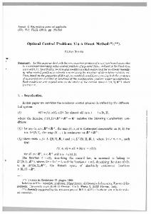
The best known optimal objective value of this problem given is given by T = 3.78086. The corresponding solution is shown in Figure 1 (right), another local minimum is plotted in Figure 1 (left). The solution of bangbang type switches three resp. five times, starting with w(t) = 1.

Fig. 1. Trajectories for the F-8 flight control problem. Left: corresponding to the Sager[53] column in Table 1. Right: corresponding to the rightmost column in Table 1.

4. Lotka Volterra Fishing Problem. The Lotka Volterra fishing problem seeks an optimal fishing strategy to be performed on a fixed time horizon to bring the biomasses of both predator as prey fish to a prescribed steady state. The problem was set up as a small-scale benchmark problem in [55] and has since been used for the evaluation of algorithms, e.g., [62]. The mathematical equations form a small-scale ODE model. The interior point equality conditions fix the initial values of the differential states. The optimal integer control shows chattering behavior, making the Lotka Volterra fishing problem an ideal candidate for benchmarking of algorithms. 4.1. Model and optimal control problem. The biomasses of two fish species — one predator, the other one prey — are the differential states of the model, the binary control is the operation of a fishing fleet.


13

The optimization goal is to penalize deviations from a steady state, Ztf min x,w

(x0 − 1)2 + (x1 − 1)2 dt

t0

s.t.

x˙ 0 = x0 − x0 x1 − c0 x0 w

(4.1)

x˙ 1 = −x1 + x0 x1 − c1 x1 w, x(0) = (0.5, 0.7)T , w(t) ∈ {0, 1},

t ∈ [0, tf ],

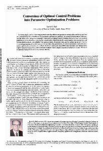
with tf = 12, c0 = 0.4, and c1 = 0.2. 4.2. Results. If the problem is relaxed, i.e., we demand that w(·) be in the continuous interval [0, 1] instead of the binary choice {0, 1}, the optimal solution can be determined by means of Pontryagin’s maximum principle [49]. The optimal solution contains a singular arc, [55]. The optimal objective value of this relaxed problem is Φ = 1.34408. As follows from MIOC theory [58] this is the best lower bound on the optimal value of the original problem with the integer restriction on the control function. In other words, this objective value can be approximated arbitrarily close, if the control only switches often enough between 0 and 1. As no optimal solution exists, a suboptimal one is shown in Figure 2, with 26 switches and an objective function value of Φ = 1.34442.

Fig. 2. Trajectories for the Lotka Volterra Fishing problem. Top left: optimal relaxed solution on grid with 52 intervals. Top right: feasible integer solution. Bottom: corresponding differential states, biomass of prey and of predator fish.

4.3. Variants. There are several alternative formulations and variants of the above problem, in particular • a prescribed time grid for the control function [55], • a time-optimal formulation to get into a steady-state [53], • the usage of a different target steady-state, as the one corresponding to w(·) = 1 which is (1 + c1 , 1 − c0 ), • different fishing control functions for the two species, • different parameters and start values. 5. Fuller’s problem. The first control problem with an optimal chattering solution was given by [22]. An optimal trajectory does exist for all initial and terminal values in a vicinity of the origin. As Fuller showed, this

14

SEBASTIAN SAGER

optimal trajectory contains a bang-bang control function that switches infinitely often. The mathematical equations form a small-scale ODE model. The interior point equality conditions fix initial and terminal values of the differential states, the objective is of tracking type. 5.1. Model and optimal control problem. The MIOCP reads as Z 1 x20 dt min x,w

s.t.

0

x˙ 0 = x1

(5.1)

x˙ 1 = 1 − 2 w x(0) = (0.01, 0)T , w(t) ∈ {0, 1},

x(T ) = (0.01, 0)T ,

t ∈ [0, 1].

5.2. Results. The optimal trajectories for the relaxed control problem on an equidistant grid G 0 with nms = 20, 30, 60 are shown in the top row of Figure 3. Note that this solution is not bang–bang due to the discretization of the control space. Even if this discretization is made very fine, a trajectory with w(·) = 0.5 on an interval in the middle of [0, 1] will be found as a minimum. The application of MS MINTOC [54] yields an objective value of Φ = 1.52845 · 10−5 , which is better than the limit of the relaxed problems, Φ20 = 1.53203 · 10−5 , Φ30 = 1.53086 · 10−5 , and Φ60 = 1.52958 · 10−5 .

Fig. 3. Trajectories for Fuller’s problem. Top row and bottom left: relaxed optima for 20, 30, and 60 equidistant control intervals. Bottom right: feasible integer solution.

5.3. Variants. An extensive analytical investigation of this problem and a discussion of the ubiquity of Fuller’s problem can be found in [63]. 6. Subway ride. The optimal control problem we treat in this section goes back to work of [9] for the city of New York. In an extension, also velocity limits that lead to path–constrained arcs appear. The aim is to minimize the energy used for a subway ride from one station to another, taking into account boundary conditions and a restriction on the time.


15

6.1. Model and optimal control problem. The MIOCP reads as Z min

tf

L(x, w) dt

x,w

0

s.t.

x˙ 0 = x1

(6.1)

x˙ 1 = f1 (x, w) x(0) = (0, 0)T ,

x(tf ) = (2112, 0)T ,

w(t) ∈ {1, 2, 3, 4},

t ∈ [0, tf ].

The terminal time tf = 65 denotes the time of arrival of a subway train in the next station. The differential states x0 (·) and x1 (·) describe position and velocity of the train, respectively. The train can be operated in one of four different modes, w(·) = 1 series, w(·) = 2 parallel, w(·) = 3 coasting, or w(·) = 4 braking that accelerate or decelerate the train and have different energy consumption. Acceleration and energy comsumption are velocitydependent. Hence, we will need switching functions σi (x1 ) = vi − x1 for given velocities vi , i = 1..3. The Lagrange term reads as  

e p1 e p2 L(x, 1) = −i  P5 1 e i=0 ci (1) 10 γ x1  ∞  e p3 L(x, 2) = −i  P5 1 e i=0 ci (2) 10 γ x1 − 1

if σ1 ≥ 0 else if σ2 ≥ 0 else

(6.2)


(6.3)

L(x, 3) = L(x, 4) = 0.

(6.4)

The right hand side function f1 (x, w) reads as

f1 (x, 1) =

f1 (x, 2) =

     f 1C 1   

f12C

f11A := gWeeffa1 f11B := gWeeffa2 1 ,1)−R(x1 ) := g (e T (xW eff


(6.5)

0 f12B := gWeeffa3 1 ,2)−R(x1 ) := g (e T (xW eff


(6.6)

g R(x1 ) − C, Weff f1 (x, 4) = −u = −umax . f1 (x, 3) = −

(6.7) (6.8)

The braking deceleration u(·) can be varied between 0 and a given umax . It can be shown that for problem (6.1) only maximal braking can be optimal,

16

SEBASTIAN SAGER

Symbol W Weff S S4 S5 γ a nwag b C g e

Value 78000 85200 2112 700 1200 3600 5280

100 10 0.045 0.367 32.2 1.0

Unit lbs lbs ft ft ft sec / ft h mile2 ft ft sec2 -

Symbol v1 v2 v3 v4 v5 a1 a2 a3 umax p1 p2 p3

Value 0.979474 6.73211 14.2658 22.0 24.0 6017.611205 12348.34865 11124.63729 4.4 106.1951102 180.9758408 354.136479

Unit mph mph mph mph mph lbs lbs lbs ft / sec2 -

Table 2 Parameters used for the subway MIOCP and its variants.

hence we fixed u(·) to umax without loss of generality. Occurring forces are 1.3 W + 116, R(x1 ) = ca γ 2 x1 2 + bW γx1 + 2000 −i 5 X 1 T (x1 , 1) = bi (1) γx1 − 0.3 , 10 i=0 −i 5 X 1 bi (2) T (x1 , 2) = γx1 − 1 . 10 i=0

(6.9) (6.10)

(6.11)

Parameters are listed in Table 2, while bi (w) and ci (w) are given by b0 (1) −0.1983670410E02, b1 (1) 0.1952738055E03, b2 (1) 0.2061789974E04, b3 (1) −0.7684409308E03, b4 (1) 0.2677869201E03, b5 (1) −0.3159629687E02, b0 (2) −0.1577169936E03, b1 (2) 0.3389010339E04, b2 (2) 0.6202054610E04, b3 (2) −0.4608734450E04, b4 (2) 0.2207757061E04, b5 (2) −0.3673344160E03, Details about the derivation of can be found in [9] or in [37].

c0 (1) 0.3629738340E02, c1 (1) −0.2115281047E03, c2 (1) 0.7488955419E03, c3 (1) −0.9511076467E03, c4 (1) 0.5710015123E03, c5 (1) −0.1221306465E03, c0 (2) 0.4120568887E02, c1 (2) 0.3408049202E03, c2 (2) −0.1436283271E03, c3 (2) 0.8108316584E02, c4 (2) −0.5689703073E01, c5 (2) −0.2191905731E01. this model and the assumptions made

6.2. Results. The optimal trajectory for this problem has been calculated by means of an indirect approach in [9, 37], and based on the

17


direct multiple shooting method in [58]. The resulting trajectory is listed in Table 3. Time t 0.00000 0.63166 2.43955 3.64338 5.59988 12.6070 45.7827 46.8938 57.1600 65.0000

w(·) 1 1 1 2 2 1 3 3 4 -

f1 = f11A f11B f11C f12B f12C f11C f1 (3) f1 (3) f1 (4) −

x0 [ft] 0.0 0.453711 10.6776 24.4836 57.3729 277.711 1556.5 1600 1976.78 2112

x1 [mph] 0.0 0.979474 6.73211 8.65723 14.2658 25.6452 26.8579 26.5306 23.5201 0.0

x1 [ftps] 0.0 1.43656 9.87375 12.6973 20.9232 37.6129 39.3915 38.9115 34.4961 0.0

Energy 0.0 0.0186331 0.109518 0.147387 0.339851 0.93519 1.14569 1.14569 1.14569 1.14569

Table 3 Optimal trajectory for the subway MIOCP as calculated in [9, 37, 58].

6.3. Variants. The given parameters have to be modified to match different parts of the track, subway train types, or amount of passengers. A minimization of travel time might also be considered. The problem becomes more challenging, when additional point or path constraints are considered. First we consider the point constraint x1 ≤ v4 if x0 = S4

(6.12)

for a given distance 0 < S4 < S and velocity v4 > v3 . Note that the state x0 (·) is strictly monotonically increasing with time, as x˙ 0 = x1 > 0 for all t ∈ (0, T ). The optimal order of gears for S4 = 1200 and v4 = 22/γ with the additional interior point constraints (6.12) is 1, 2, 1, 3, 4, 2, 1, 3, 4. The stage lengths between switches are 2.86362, 10.722, 15.3108, 5.81821, 1.18383, 2.72451, 12.917, 5.47402, and 7.98594 with Φ = 1.3978. For different parameters S4 = 700 and v4 = 22/γ we obtain the gear choice 1, 2, 1, 3, 2, 1, 3, 4 and stage lengths 2.98084, 6.28428, 11.0714, 4.77575, 6.0483, 18.6081, 6.4893, and 8.74202 with Φ = 1.32518. A more practical restriction are path constraints on subsets of the track. We will consider a problem with additional path constraints x1 ≤ v5 if x0 ≥ S5 .

(6.13)

The additional path constraint changes the qualitative behavior of the relaxed solution. While all solutions considered this far were bang–bang and the main work consisted in finding the switching points, we now have a path–constraint arc. The optimal solutions for refined grids yield a series of monotonically decreasing objective function values, where the limit is

18

SEBASTIAN SAGER

Optimal solution with 1 touch point

Optimal solution with 3 touch points

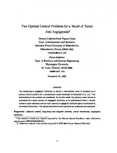
Fig. 4. The differential state velocity of a subway train over time. The dotted vertical line indicates the beginning of the path constraint, the horizontal line the maximum velocity. Left: one switch leading to one touch point. Right: optimal solution for three switches. The energy-optimal solution needs to stay as close as possible to the maximum velocity on this time interval to avoid even higher energy-intensive accelerations in the start-up phase to match the terminal time constraint tf ≤ 65 to reach the next station.

the best value that can be approximated by an integer feasible solution. In our case we obtain 1.33108, 1.31070, 1.31058, 1.31058, . . .

(6.14)

Figure 4 shows two possible integer realizations, with a trade-off between energy consumption and number of switches. Note that the solutions approximate the optimal driving behavior (a convex combination of two operation modes) by switching between the two and causing a touching of the velocity constraint from below as many times as we switch. 7. Resetting calcium oscillations. The aim of the control problem is to identify strength and timing of inhibitor stimuli that lead to a phase singularity which annihilates intra-cellular calcium oscillations. This is formulated as an objective function that aims at minimizing the state deviation from a desired unstable steady state, integrated over time. A calcium oscillator model describing intra-cellular calcium spiking in hepatocytes induced by an extracellular increase in adenosine triphosphate (ATP) concentration is described. The calcium signaling pathway is initiated via a receptor activated G-protein inducing the intra-cellular release of


19

inositol triphosphate (IP3) by phospholipase C. The IP3 triggers the opening of endoplasmic reticulum and plasma membrane calcium channels and a subsequent inflow of calcium ions from intra-cellular and extracellular stores leading to transient calcium spikes. The mathematical equations form a small-scale ODE model. The interior point equality conditions fix the initial values of the differential states. The problem is, despite of its low dimension, very hard to solve, as the target state is unstable. 7.1. Model and optimal control problem. The MIOCP reads as Z minmax

x,w,w

s.t.

tf

||x(t) − x ˜||22 + p1 w(t) dt

0

k5 x0 x2 k3 x0 x1 − x0 + K4 x0 + K6 k8 x1 x˙ 1 = k7 x0 − x1 + K9 k10 x1 x2 x3 k14 x2 x˙ 2 = + k12 x1 + k13 x0 − x3 + K11 w · x2 + K15 k16 x2 x3 − + x2 + K17 10 k10 x1 x2 x3 k16 x2 x3 x˙ 3 = − + − x3 + K11 x2 + K17 10 x(0) = (0.03966, 1.09799, 0.00142, 1.65431)T , x˙ 0 = k1 + k2 x0 −

(7.1)

1.1 ≤ wmax ≤ 1.3, w(t) ∈ {1, wmax }, t ∈ [0, tf ] with fixed parameter values [t0 , tf ] = [0, 22], k1 = 0.09, k2 = 2.30066, k3 = 0.64, K4 = 0.19, k5 = 4.88, K6 = 1.18, k7 = 2.08, k8 = 32.24, K9 = 29.09, k10 = 5.0, K11 = 2.67, k12 = 0.7, k13 = 13.58, k14 = 153.0, K15 = 0.16, k16 = 4.85, K17 = 0.05, p1 = 100, and reference values x ˜0 = 6.78677, x ˜1 = 22.65836, x ˜2 = 0.384306, x ˜3 = 0.28977. The differential states (x0 , x1 , x2 , x3 ) describe concentrations of activated G-proteins, active phospholipase C, intra-cellular calcium, and intraER calcium, respectively. The external control w(·) is a temporally varying concentration of an uncompetitive inhibitor of the PMCA ion pump. Modeling details can be found in [38]. In the given equations that stem from [40], the model is identical to the one derived there, except for an additional first-order leakage flow of calcium from the ER back to the cytoplasm, which is modeled by x103 . It reproduces well experimental observations of cytoplasmic calcium oscillations as well as bursting behavior and in particular the frequency encoding of the triggering stimulus strength, which is a well known mechanism for signal processing in cell biology.

20

SEBASTIAN SAGER

7.2. Results. The depicted optimal solution in Figure 5 consists of a stimulus of wmax = 1.3 and a timing given by the stage lengths 4.6947115, 0.1491038, and 17.1561845. The optimal objective function value is Φ = 1610.654. As can be seen from the additional plots, this solution is extremely unstable. A small perturbation in the control, or simply rounding errors on a longer time horizon lead to a transition back to the stable limit-cycle oscillations. The determination of the stimulus by means of optimization is quite hard for two reasons. First, the unstable target steady-state. Only a stable all-at-once algorithm such as multiple shooting or collocation can be applied successfully. Second, the objective landscape of the problem in switching time formulation (this is, for a fixed stimulus strength and modifying only beginning and length of the stimulus) is quite nasty, as the visualizations in [53] and on the web page [52] show.

Fig. 5. Trajectories for the calcium problem. Top left: optimal integer solution. Top right: corresponding differential states with phase resetting. Bottom left: slightly perturbed control: stimulus 0.001 too early. Bottom right: long time behavior of optimal solution: numerical rounding errors lead to transition back from unstable steady-state to stable limit-cycle.

7.3. Variants. Alternatively, also the annihilation of calcium oscillations with PLC activation inhibition, i.e., the use of two control functions is possible, compare [40]. Of course, results depend very much on the scaling of the deviation in the objective function.


21

8. Supermarket refrigeration system. This benchmark problem was formulated first within the European network of excellence HYCON, [45] by Larsen et. al, [39]. The formulation lacks however a precise definition of initial values and constraints, which are only formulated as “soft constraints”. The task is to control a refrigeration system in an energy optimal way, while guaranteeing safeguards on the temperature of the showcases. This problem would typically be a moving horizon online optimization problem, here it is defined as a fixed horizon optimization task. The mathematical equations form a periodic ODE model. 8.1. Model and optimal control problem. The MIOCP reads as Z 1 tf (w2 + w3 ) · 0.5 · ηvol · Vsl · f dt min x,w,tf tf 0 x4 x2 − Te (x0 ) + x8 x6 − Te (x0 ) U Awrm s.t. x˙ 0 = · dρsuc Mrm · ∆hlg (x0 ) Vsuc · dPsuc (x0 ) + x˙ 1 = −

Mrc − ηvol · Vsl · 0.5 (w2 + w3 ) ρsuc (x0 ) dρsuc (x0 ) Vsuc · dP suc U Agoods−air (x1 − x3 ) Mgoods · Cp,goods

U Awrm x4 x2 − Te (x0 ) Mrm = Mwall · Cp,wall U Agoods−air (x1 − x3 ) + Q˙ airload − U Aair−wall (x3 − x2 ) = Mair · Cp,air Mrm − x4 U Awrm (1 − w0 ) = x4 x2 − Te (x0 ) w0 − τf ill Mrm · ∆hlg (x0 ) U Agoods−air (x5 − x7 ) =− Mgoods · Cp,goods U Awrm U Aair−wall (x7 − x6 ) − x8 x6 − Te (x0 ) Mrm = Mwall · Cp,wall U Agoods−air (x5 − x7 ) + Q˙ airload − U Aair−wall (x7 − x6 ) = Mair · Cp,air U Awrm (1 − w1 ) Mrm − x8 w1 − x8 x6 − Te (x0 ) = τf ill Mrm · ∆hlg (x0 ) U Aair−wall (x3 − x2 ) −

x˙ 2 x˙ 3 x˙ 4 x˙ 5

x˙ 6 x˙ 7 x˙ 8

x(0) = x(tf ), 650 ≤ tf ≤ 750, x0 ≤ 1.7, 2 ≤ x3 ≤ 5, 2 ≤ x7 ≤ 5 w(t) ∈ {0, 1}4 ,

t ∈ [0, tf ].

22

SEBASTIAN SAGER

Symbol Q˙ airload m ˙ rc Mgoods Cp,goods U Agoods−air Mwall Cp,wall U Aair−wall Mair Cp,air U Awrm τf ill TSH Mrm Vsuc Vsl ηvol

Value 3000.00 0.20 200.00 1000.00 300.00 260.00 385.00 500.00 50.00 1000.00 4000.00 40.00 10.00 1.00 5.00 0.08 0.81

Unit J s kg s

kg J kg·K J s·K

kg J kg·K J s·K

kg J kg·K J s·K

s K kg m3 m3 s

−

Description Disturbance, heat transfer Disturbance, constant mass flow Mass of goods Heat capacity of goods Heat transfer coefficient Mass of evaporator wall Heat capacity of evaporator wall Heat transfer coefficient Mass of air in display case Heat capacity of air Maximum heat transfer coefficient Filling time of the evaporator Superheat in the suction manifold Maximum mass of refrigerant Total volume of suction manifold Total displacement volume Volumetric efficiency

Table 4 Parameters used for the supermarket refrigeration problem.

The differential state x0 describes the suction pressure in the suction manifold (in bar). The next three states model temperatures in the first display case (in C). x1 is the goods’ temperature, x2 the one of the evaporator wall and x3 the air temperature surrounding the goods. x4 then models the mass of the liquefied refrigerant in the evaporator (in kg). x5 to x8 describe the corresponding states in the second display case. w0 and w1 describe the inlet valves of the first two display cases, respectively. w2 and w3 denote the activity of a single compressor. The model uses the parameter values listed in Table 4 and the polynomial functions obtained from interpolations: Te (x0 ) = −4.3544x20 + 29.224x0 − 51.2005, ∆hlg (x0 ) = (0.0217x20 − 0.1704x0 + 2.2988) · 105 , ρsuc (x0 ) = 4.6073x0 + 0.3798, dρsuc 3 2 dPsuc (x0 ) = −0.0329x0 + 0.2161x0 − 0.4742x0 + 5.4817. 8.2. Results. For the relaxed problem the optimal solution is Φ = 12072.45. The integer solution plotted in Figure 6 is feasible, but yields an increased objective function value of Φ = 12252.81, a compromise between effectiveness and a reduced number of switches. 8.3. Variants. Since the compressors are parallel connected one can introduce a single control w2 ∈ {0, 1, 2} instead of two equivalent controls. The same holds for scenarios with n parallel connected compressors.


23

Fig. 6. Periodic trajectories for optimal relaxed (left) and integer feasible controls (right), with the controls w(·) in the first row and the differential states in the three bottom rows.

In [39], the problem was stated slightly different: • The temperature constraints weren’t hard bounds but there was a penalization term added to the objective function to minimize the violation of these constraints. • The differential equation for the mass of the refrigerant had another switch, if the valve (e.g. w0 ) is closed. It was formulated as x˙4 = Mrm − x4 U Awrm x4 x2 − Te (x0 ) if if w0 = 1, x˙4 = − τf ill Mrm · ∆hlg (x0 ) w0 = 0 and x4 > 0, or x˙4 = 0 if w0 = 0 and x4 = 0. This additional switch is redundant because the mass itself is a factor on the right hand side and so the complete right hand side is 0 if x4 = 0. • A night scenario with two different parameters was given. At night the following parameters change their value to Q˙ airload = 1800.00 Js and m ˙ rc = 0.00 kg s . Additionally the constraint on the suction pressure x0 (t) is softened to x0 (t) ≤ 1.9. • The number of compressors and display cases is not fixed. Larsen also proposed the problem with 3 compressors and 3 display cases. This leads to a change in the compressor rack’s performance to 3 Vsl = 0.095 ms . Unfortunately this constant is only given for these two cases although Larsen proposed scenarios with more compressors and display cases. 9. Elchtest testdrive. We consider a time-optimal car driving maneuver to avoid an obstacle with small steering effort. At any time, the car must be positioned on a prescribed track. This control problem was first formulated in [24] and used for subsequent studies [25, 36]. The mathematical equations form a small-scale ODE model. The in-

24

SEBASTIAN SAGER

terior point equality conditions fix initial and terminal values of the differential states, the objective is of minimum-time type.

9.1. Model and optimal control problem. We consider a car model derived under the simplifying assumption that rolling and pitching of the car body can be neglected. Only a single front and rear wheel is modelled, located in the virtual center of the original two wheels. Motion of the car body is considered on the horizontal plane only. The MIOCP reads as Z

min tf ,x(·),u(·)

s.t.

tf

wδ2 (t) dt c˙x = v cos ψ − β c˙y = v sin ψ − β 1 µ (Flr − FAx ) cos β + Flf cos δ + β v˙ = m − (Fsr − FAy ) sin β − Fsf sin δ + β tf +

(9.1a)

0

δ˙ = wδ

(9.1c) (9.1d)

(9.1e)

1 β˙ = wz − (Flr − FAx ) sin β + Flf sin δ + β mv + (Fsr − FAy ) cos β + Fsf cos δ + β ψ˙ = wz 1 Fsf lf cos δ − Fsr lr − FAy eSP + Flf lf sin δ w˙z = I zz cy (t) ∈ Pl (cx (t)) + B2 , Pu (cx (t)) − B2 wδ (t) ∈ [−0.5, 0.5],

(9.1b)

4

FB (t) ∈ [0, 1.5 · 10 ],

φ(t) ∈ [0, 1]

µ(t) ∈ {1, . . . , 5} | x(t0 ) = −30, free, 10, 0, 0, 0, 0 ,

(9.1f)

(9.1g) (9.1h) (9.1i) (9.1j) (9.1k)

(cx , ψ)(tf ) = (140, 0)

(9.1l)

for t ∈ [t0 , tf ] almost everywhere. The four control functions contained in u(·) are steering wheel angular velocity wδ , total braking force FB , the accelerator pedal position φ and the gear µ. The differential states contained in x(·) are horizontal position of the car cx , vertical position of the car cy , magnitude of directional velocity of the car v, steering wheel angle δ, side slip angle β, yaw angle ψ, and the y aw angle velocity wz . The model parameters are listed in Table 5, while the forces and ex-

25


pressions in (9.1b) to (9.1h) are given for fixed µ by Fsf,sr (αf,r ) := Df,r sin Cf,r arctan Bf,r αf,r − Ef,r (Bf,r αf,r − arctan(Bf,r αf,r )) ! ˙ − v(t) sin β(t) lf ψ(t) αf := δ(t) − arctan v(t) cos β(t) ! ˙ + v(t) sin β(t) lr ψ(t) αr := arctan , v(t) cos β(t)

,

Flf := −FBf − FRf , iµg it µ Mmot (φ) − FBr − FRr , Flrµ := R µ µ µ ), Mmot (φ) := f1 (φ) f2 (wmot ) + (1 − f1 (φ)) f3 (wmot f1 (φ) := 1 − exp(−3 φ), 2 f2 (wmot ) := −37.8 + 1.54 wmot − 0.0019 wmot ,

f3 (wmot ) := −34.9 − 0.04775 wmot , iµg it µ wmot := v(t), R 2 1 FBf := FB , FBr := FB , 3 3 m lr g m lf g FRf (v) := fR (v) , FRr (v) := fR (v) , lf + lr lf + lr fR (v) := 9 · 10−3 + 7.2 · 10−5 v + 5.038848 · 10−10 v 4 , 1 FAy := 0. FAx := cw ρ A v 2 (t), 2

The test track is described by setting up piecewise cubic spline functions Pl (x) and Pr (x) modeling the top and bottom track boundary, given a horizontal position x.

 0     4 h2 (x − 44)3      4 h2 (x − 45)3 + h2 h2 Pl (x) :=   4 h2 (70 − x)3 + h2     4 h2 (71 − x)3    0

if if if if if if if

44 < 44.5 < 45 < 70 < 70.5 < 71
0; # param nt > 0; # param nu > 0; # param nx > 0; # param n t p e r u > 0 ; # s e t I := 0 . . nt ; s e t U:= 0 . . nu −1; param u i d x { I } ; param

End time Number o f d i s c r e t i z a t i o n p o i n t s i n time Number o f c o n t r o l d i s c r e t i z a t i o n p o i n t s Dimension o f d i f f e r e n t i a l s t a t e v e c t o r n t / nu

f i x w ; param f i x w ;

var w {U} >= 0 , = 0 , 0 )

t h e n { f o r { i in U} { f i x w [ i ] ; } }

34 if

SEBASTIAN SAGER ( f i x dt > 0 ) t h e n { f o r { i in U} { f i x dt [ i ] ; } }

# S e t i n d i c e s o f c o n t r o l s c o r r e s p o n d i n g t o time p o i n t s f o r { i in 0 . . nu−1} { f o r { j in 0 . . n t p e r u −1} { l e t u i d x [ i ∗ n t p e r u+j ] := i ; } } l e t u i d x [ nt ] := nu −1;

12.2. Lotka Volterra Fishing Problem. The AMPL code in Listings 3 and 4 shows a discretization of the problem(4.1) with piecewise constant controls on an equidistant grid of length T /nu and with an implicit Euler method. Note that for other MIOCPs, especially for unstable ones as in Section 7, more advanced integration methods such as Backward Differentiation Formulae need to be applied. Listing 3 AMPL model file for Lotka Volterra Fishing Problem var x { I , 1 . . nx} >= 0 ; param c1 > 0 ; param c2 > 0 ; param r e f 1 > 0 ; param r e f 2 > 0 ; minimize D e v i a t i o n : 0 . 5 ∗ ( dt [ 0 ] / n t p e r u ) ∗ ( ( x [ 0 , 1 ] − r e f 1 ) ˆ 2 + ( x [ 0 , 2 ] − r e f 2 ) ˆ 2 ) + 0 . 5 ∗ ( dt [ nu −1]/ n t p e r u ) ∗ ( ( x [ nt , 1 ] − r e f 1 ) ˆ 2 + ( x [ nt , 2 ] − r e f 2 ) ˆ 2 ) + sum { i in I d i f f { 0 , nt } } ( ( dt [ u i d x [ i ] ] / n t p e r u ) ∗ ( ( x [ i , 1 ] − r e f 1 )ˆ2 + ( x [ i , 2 ] − r e f 2 )ˆ2 ) ) ; subj to ODE DISC 1 { i in I d i f f { 0 } } : x [ i , 1 ] = x [ i − 1 , 1 ] + ( dt [ u i d x [ i ] ] / n t p e r u ) ∗ ( x [ i , 1 ] − x [ i , 1 ] ∗x [ i , 2 ] − x [ i , 1 ] ∗ c1 ∗w [ u i d x [ i ] ]

);

subj to ODE DISC 2 { i in I d i f f { 0 } } : x [ i , 2 ] = x [ i − 1 , 2 ] + ( dt [ u i d x [ i ] ] / n t p e r u ) ∗ ( − x [ i , 2 ] + x [ i , 1 ] ∗x [ i , 2 ] − x [ i , 2 ] ∗ c2 ∗w [ u i d x [ i ] ]

);

subj to o v e r a l l s t a g e l e n g t h : sum { i in U} dt [ i ] = T ;

Listing 4 AMPL dat file for Lotka Volterra Fishing Problem # A l g o r i t h m i c pa r am et er s param n t p e r u := 1 0 0 ; param nu := 1 0 0 ; param nt := 1 0 0 0 0 ; param nx := 2 ; param f i x w := 0 ; param f i x dt := 1 ; # Problem pa ra me te r s param T := 1 2 . 0 ; param c1 := 0 . 4 ; param c2 := 0 . 2 ; param r e f 1 := 1 . 0 ; param r e f 2 := 1 . 0 ; # I n i t i a l values d i f f e r e n t i a l states l e t x [ 0 , 1 ] := 0 . 5 ; l e t x [ 0 , 2 ] := 0 . 7 ; fix x [ 0 , 1 ] ; fix x [ 0 , 2 ] ; # Initial l e t { i in f o r { i in l e t { i in

values control U} w [ i ] := 0 . 0 ; 0 . . ( nu−1) / 2} { l e t w [ i ∗ 2 ] := 1 . 0 ; } U} dt [ i ] := T / nu ;

Note that the constraint overall stage length is only necessary, when the value for fix dt is zero, a switching time optimization. The solution calculated by Bonmin (subversion revision number 1453, default settings, 3 GHz, Linux 2.6.28-13-generic, with ASL(20081205)) has


35

an objective function value of Φ = 1.34434, while the optimum of the relaxation is Φ = 1.3423368. Bonmin needs 35301 iterations and 2741 nodes (4899.97 seconds). The intervals on the equidistant grid on which w(t) = 1 holds, counting from 0 to 99, are 20–32, 34, 36, 38, 40, 44, 53. 12.3. F-8 flight control. The main difficulty in calculating a timeoptimal solution for the problem in Section 3 is the determination of the correct switching structure and of the switching points. If we want to formulate a MINLP, we have to slightly modify this problem. Our aim is not a minimization of the overall time, but now we want to get as close as possible to the origin (0, 0, 0) in a prespecified time tf = 3.78086 on an equidistant time grid. As this time grid is not a superset of the one used for the time-optimal solution in Section 3, one can not expect to reach the target state exactly. Listings 5 and 6 show the AMPL code. Listing 5 AMPL model file for F-8 Flight Control Problem var x { I , param x i

1 . . nx } ; > 0;

minimize D e v i a t i o n : sum { i in 1 . . 3 } x [ nt , i ] ∗x [ nt , i ] ; subj to ODE DISC 1 { i in I d i f f { 0 } } : x [ i , 1 ] = x [ i − 1 , 1 ] + ( dt [ u i d x [ i ] ] / n t p e r u ) ∗ ( − 0 . 8 7 7 ∗x [ i , 1 ] + x [ i , 3 ] − 0 . 0 8 8 ∗x [ i , 1 ] ∗x [ i , 3 ] + 0 . 4 7 ∗x [ i , 1 ] ∗x [ i , 1 ] − 0 . 0 1 9 ∗x [ i , 2 ] ∗x [ i , 2 ] − x [ i , 1 ] ∗x [ i , 1 ] ∗x [ i , 3 ] + 3 . 8 4 6 ∗x [ i , 1 ] ∗x [ i , 1 ] ∗x [ i , 1 ] + 0 . 2 1 5 ∗ x i − 0 . 2 8 ∗x [ i , 1 ] ∗x [ i , 1 ] ∗ x i + 0 . 4 7 ∗x [ i , 1 ] ∗ x i ˆ2 − 0 . 6 3 ∗ x i ˆ2 − 2∗w [ u i d x [ i ] ] ∗ ( 0 . 2 1 5 ∗ x i − 0 . 2 8 ∗x [ i , 1 ] ∗x [ i , 1 ] ∗ x i − 0 . 6 3 ∗ x i ˆ 3 ) ) ; subj to ODE DISC 2 { i in I d i f f { 0 } } : x [ i , 2 ] = x [ i − 1 , 2 ] + ( dt [ u i d x [ i ] ] / n t p e r u ) ∗ x [ i , 3 ] ; subj to ODE DISC 3 { i in I d i f f { 0 } } : x [ i , 3 ] = x [ i − 1 , 3 ] + ( dt [ u i d x [ i ] ] / n t p e r u ) ∗ ( − 4 . 2 0 8 ∗x [ i , 1 ] − 0 . 3 9 6 ∗x [ i , 3 ] − 0 . 4 7 ∗x [ i , 1 ] ∗x [ i , 1 ] − 3 . 5 6 4 ∗x [ i , 1 ] ∗x [ i , 1 ] ∗x [ i , 1 ] + 2 0 . 9 6 7 ∗ x i − 6 . 2 6 5 ∗x [ i , 1 ] ∗x [ i , 1 ] ∗ x i + 46∗x [ i , 1 ] ∗ x i ˆ2 − 6 1 . 4 ∗ x i ˆ3 − 2∗w [ u i d x [ i ] ] ∗ ( 2 0 . 9 6 7 ∗ x i − 6 . 2 6 5 ∗x [ i , 1 ] ∗x [ i , 1 ] ∗ x i − 6 1 . 4 ∗ x i ˆ 3 ) ) ;

Listing 6 AMPL dat file for F-8 Flight Control Problem # Parameters param n t p e r u := 5 0 0 ; param nx := 3 ; param x i := 0 . 0 5 2 3 6 ;

param nu := 6 0 ; param nt := 3 0 0 0 0 ; param f i x w := 0 ; param f i x dt := 1 ; param T := 8 ;

# Initial let x [0 ,1] let x [0 ,2] let x [0 ,3] f o r { i in

values d i f f e r e n t i a l states := 0 . 4 6 5 5 ; := 0 . 0 ; := 0 . 0 ; 1..3} { fix x [0 , i ] ; }

# Initial l e t { i in f o r { i in l e t { i in

values control U} w [ i ] := 0 . 0 ; 0 . . ( nu−1) / 2} { l e t w [ i ∗ 2 ] := 1 . 0 ; } U} dt [ i ] := 3 . 7 8 0 8 6 / nu ;

The solution calculated by Bonmin has an objective function value of Φ = 0.023405, while the optimum of the relaxation is Φ = 0.023079. Bonmin

36

SEBASTIAN SAGER

needs 85702 iterations and 7031 nodes (64282 seconds). The intervals on the equidistant grid on which w(t) = 1 holds, counting from 0 to 59, are 0, 1, 31, 32, 42, 52, and 54. This optimal solution is shown in Figure 10.

Fig. 10. Trajectories for the discretized F-8 flight control problem. Left: optimal integer control. Right: corresponding differential states.

13. Conclusions and outlook. We presented a collection of mixedinteger optimal control problem descriptions. These descriptions comprise details on the model and a specific instance of control objective, constraints, parameters, and initial values that yield well-posed optimization problems that allow for reproducibility and comparison of solutions. Furthermore, specific discretizations in time and space are applied with the intention to supply benchmark problems also for MINLP algorithm developers. The descriptions are complemented by references and best known solutions. All problem formulations are or will be available for download at http://mintoc.de in a suited format, such as optimica or AMPL. The author hopes to achieve at least two things. First, to provide a benchmark library that will be of use for both MIOC and MINLP algorithm developers. Second, to motivate others to contribute to the extension of this library. For example, challenging and well-posed instances from water or gas networks [11, 44], traffic flow [30, 21], supply chain networks [26], submarine control [51], distributed autonomous systems [1], and chemical engineering [34, 60] would be highly interesting for the community. Acknowledgements. Important contributions to the online resource http://mintoc.de by Alexander Buchner, Michael Engelhart, Christian Kirches, and Martin Schl¨ uter are gratefully acknowledged. REFERENCES [1] P. Abichandani, H. Benson, and M. Kam, Multi-vehicle path coordination under communication constraints, in American Control Conference, 2008, pp. 650– 656. [2] W. Achtziger and C. Kanzow, Mathematical programs with vanishing constraints: optimality conditions and constraint qualifications, Mathematical Programming Series A, 114 (2008), pp. 69–99.


37

[3] E. S. Agency, GTOP database: Global optimisation trajectory problems and solutions. http://www.esa.int/gsp/ACT/inf/op/globopt.htm. [4] AT&T Bell Laboratories, University of Tennessee, and Oak Ridge National Laboratory, Netlib linear programming library. http://www.netlib.org/lp/. [5] B. Baumrucker and L. Biegler, Mpec strategies for optimization of a class of hybrid dynamic systems, Journal of Process Control, 19 (2009), pp. 1248 – 1256. Special Section on Hybrid Systems: Modeling, Simulation and Optimization. [6] B. Baumrucker, J. Renfro, and L. Biegler, Mpec problem formulations and solution strategies with chemical engineering applications, Computers and Chemical Engineering, 32 (2008), pp. 2903–2913. [7] L. Biegler, Solution of dynamic optimization problems by successive quadratic programming and orthogonal collocation, Computers and Chemical Engineering, 8 (1984), pp. 243–248. [8] T. Binder, L. Blank, H. Bock, R. Bulirsch, W. Dahmen, M. Diehl, T. Kro¨ der, and O. Stryk, Introduction to model nseder, W. Marquardt, J. Schlo based optimization of chemical processes on moving horizons, in Online Optimization of Large Scale Systems: State of the Art, M. Gr¨ otschel, S. Krumke, and J. Rambau, eds., Springer, 2001, pp. 295–340. [9] H. Bock and R. Longman, Computation of optimal controls on disjoint control sets for minimum energy subway operation, in Proceedings of the American Astronomical Society. Symposium on Engineering Science and Mechanics, Taiwan, 1982. [10] H. Bock and K. Plitt, A Multiple Shooting algorithm for direct solution of optimal control problems, in Proceedings of the 9th IFAC World Congress, Budapest, 1984, Pergamon Press, pp. 243–247. Available at http://www.iwr.uniheidelberg.de/groups/agbock/FILES/Bock1984.pdf. ¨ dig, and M. Steinbach, Nonlinear programming tech[11] J. Burgschweiger, B. Gna niques for operative planning in large drinking water networks, The Open Applied Mathematics Journal, 3 (2009), pp. 1–16. [12] M. Bussieck, Gams performance world. http://www.gamsworld.org/performance. [13] M. R. Bussieck, A. S. Drud, and A. Meeraus, Minlplib–a collection of test models for mixed-integer nonlinear programming, INFORMS J. on Computing, 15 (2003), pp. 114–119. [14] B. Chachuat, A. Singer, and P. Barton, Global methods for dynamic optimization and mixed-integer dynamic optimization, Industrial and Engineering Chemistry Research, 45 (2006), pp. 8573–8392. [15] CMU-IBM, Cyber-infrastructure for MINLP collaborative site. http://minlp.org. [16] M. Diehl and A. Walther, A test problem for periodic optimal control algorithms, tech. rep., ESAT/SISTA, K.U. Leuven, 2006. [17] S. Engell and A. Toumi, Optimisation and control of chromatography, Computers and Chemical Engineering, 29 (2005), pp. 1243–1252. [18] W. Esposito and C. Floudas, Deterministic global optimization in optimal control problems, Journal of Global Optimization, 17 (2000), pp. 97–126. [19] B. C. Fabien, dsoa: Dynamic system optimization. http://abs5.me.washington.edu/noc/dsoa.html. [20] A. Filippov, Differential equations with discontinuous right hand side, AMS Transl., 42 (1964), pp. 199–231. ¨ genschuh, M. Herty, A. Klar, and A. Martin, Combinatorial and contin[21] A. Fu uous models for the optimization of traffic flows on networks, SIAM Journal on Optimization, 16 (2006), pp. 1155–1176. [22] A. Fuller, Study of an optimum nonlinear control system, Journal of Electronics and Control, 15 (1963), pp. 63–71. [23] W. Garrard and J. Jordan, Design of nonlinear automatic control systems, Automatica, 13 (1977), pp. 497–505. [24] M. Gerdts, Solving mixed-integer optimal control problems by Branch&Bound:

38

[25] [26]

[27] [28] [29]

[30]

[31] [32]

[33]

[34] [35] [36]

[37]

[38]

[39]

[40]

[41]

[42]

[43] [44]

SEBASTIAN SAGER A case study from automobile test-driving with gear shift, Optimal Control Applications and Methods, 26 (2005), pp. 1–18. , A variable time transformation method for mixed-integer optimal control problems, Optimal Control Applications and Methods, 27 (2006), pp. 169–182. ¨ ttlich, M. Herty, C. Kirchner, and A. Klar, Optimal control for conS. Go tinuous supply network models, Networks and Heterogenous Media, 1 (2007), pp. 675–688. N. Gould, D. Orban, and P. Toint, CUTEr testing environment for optimization and linear algebra solvers. http://cuter.rl.ac.uk/cuter-www/. I. Grossmann, Review of nonlinear mixed-integer and disjunctive programming techniques, Optimization and Engineering, 3 (2002), pp. 227–252. I. Grossmann, P. Aguirre, and M. Barttfeld, Optimal synthesis of complex distillation columns using rigorous models, Computers and Chemical Engineering, 29 (2005), pp. 1203–1215. M. Gugat, M. Herty, A. Klar, and G. Leugering, Optimal control for traffic flow networks, Journal of Optimization Theory and Applications, 126 (2005), pp. 589–616. T. O. Inc., Propt - matlab optimal control software (dae, ode). http://tomdyn.com/. A. Izmailov and M. Solodov, Mathematical programs with vanishing constraints: Optimality conditions, sensitivity, and a relaxation method, Journal of Optimization Theory and Applications, 142 (2009), pp. 501–532. Y. Kawajiri and L. Biegler, A nonlinear programming superstructure for optimal dynamic operations of simulated moving bed processes, I&EC Research, 45 (2006), pp. 8503–8513. , Optimization strategies for Simulated Moving Bed and PowerFeed processes, AIChE Journal, 52 (2006), pp. 1343–1350. C. Kaya and J. Noakes, A computational method for time-optimal control, Journal of Optimization Theory and Applications, 117 (2003), pp. 69–92. ¨ der, Time-optimal control of autoC. Kirches, S. Sager, H. Bock, and J. Schlo mobile test drives with gear shifts, Optimal Control Applications and Methods, (2010). DOI 10.1002/oca.892. ¨ mer-Eis, Ein Mehrzielverfahren zur numerischen Berechnung optimaler P. Kra Feedback–Steuerungen bei beschr¨ ankten nichtlinearen Steuerungsproblemen, vol. 166 of Bonner Mathematische Schriften, Universit¨ at Bonn, Bonn, 1985. U. Kummer, L. Olsen, C. Dixon, A. Green, E. Bornberg-Bauer, and G. Baier, Switching from simple to complex oscillations in calcium signaling, Biophysical Journal, 79 (2000), pp. 1188–1195. L. Larsen, R. Izadi-Zamanabadi, R. Wisniewski, and C. Sonntag, Supermarket refrigeration systems – a benchmark for the optimal control of hybrid systems, tech. rep., Technical report for the HYCON NoE., 2007. http://www.bci.tudortmund.de/ast/hycon4b/index.php. D. Lebiedz, S. Sager, H. Bock, and P. Lebiedz, Annihilation of limit cycle oscillations by identification of critical phase resetting stimuli via mixed-integer optimal control methods, Physical Review Letters, 95 (2005), p. 108303. H. Lee, K. Teo, V. Rehbock, and L. Jennings, Control parametrization enhancing technique for time-optimal control problems, Dynamic Systems and Applications, 6 (1997), pp. 243–262. D. Leineweber, Efficient reduced SQP methods for the optimization of chemical processes described by large sparse DAE models, vol. 613 of FortschrittBerichte VDI Reihe 3, Verfahrenstechnik, VDI Verlag, D¨ usseldorf, 1999. A. Martin, T. Achterberg, T. Koch, and G. Gamrath, Miplib - mixed integer problem library. http://miplib.zib.de/. ¨ ller, and S. Moritz, Mixed integer models for the stationary A. Martin, M. Mo case of gas network optimization, Mathematical Programming, 105 (2006), pp. 563–582.


39

[45] E. N. of Excellence Hybrid Control, Website. http://www.ist-hycon.org/. [46] J. Oldenburg, Logic–based modeling and optimization of discrete–continuous dynamic systems, vol. 830 of Fortschritt-Berichte VDI Reihe 3, Verfahrenstechnik, VDI Verlag, D¨ usseldorf, 2005. [47] J. Oldenburg and W. Marquardt, Disjunctive modeling for optimal control of hybrid systems, Computers and Chemical Engineering, 32 (2008), pp. 2346– 2364. [48] I. Papamichail and C. Adjiman, Global optimization of dynamic systems, Computers and Chemical Engineering, 28 (2004), pp. 403–415. [49] L. Pontryagin, V. Boltyanski, R. Gamkrelidze, and E. Miscenko, The Mathematical Theory of Optimal Processes, Wiley, Chichester, 1962. [50] A. Prata, J. Oldenburg, A. Kroll, and W. Marquardt, Integrated scheduling and dynamic optimization of grade transitions for a continuous polymerization reactor, Computers and Chemical Engineering, 32 (2008), pp. 463–476. [51] V. Rehbock and L. Caccetta, Two defence applications involving discrete valued optimal control, ANZIAM Journal, 44 (2002), pp. E33–E54. [52] S. Sager, MIOCP benchmark site. http://mintoc.de. [53] S. Sager, Numerical methods for mixed–integer optimal control problems, Der andere Verlag, T¨ onning, L¨ ubeck, Marburg, 2005. ISBN 3-89959-416-9. Available at http://sager1.de/sebastian/downloads/Sager2005.pdf. [54] S. Sager, Reformulations and algorithms for the optimization of switching decisions in nonlinear optimal control, Journal of Process Control, 19 (2009), pp. 1238–1247. ¨ der, Numerical methods [55] S. Sager, H. Bock, M. Diehl, G. Reinelt, and J. Schlo for optimal control with binary control functions applied to a Lotka-Volterra type fishing problem, in Recent Advances in Optimization (Proceedings of the 12th French-German-Spanish Conference on Optimization), A. Seeger, ed., vol. 563 of Lectures Notes in Economics and Mathematical Systems, Heidelberg, 2006, Springer, pp. 269–289. ¨ pper, and S. Engell, Determining SMB [56] S. Sager, M. Diehl, G. Singh, A. Ku superstructures by mixed-integer control, in Proceedings OR2006, K.-H. Waldmann and U. Stocker, eds., Karlsruhe, 2007, Springer, pp. 37–44. [57] S. Sager, C. Kirches, and H. Bock, Fast solution of periodic optimal control problems in automobile test-driving with gear shifts, in Proceedings of the 47th IEEE Conference on Decision and Control (CDC 2008), Cancun, Mexico, 2008, pp. 1563–1568. ISBN: 978-1-4244-3124-3. [58] S. Sager, G. Reinelt, and H. Bock, Direct methods with maximal lower bound for mixed-integer optimal control problems, Mathematical Programming, 118 (2009), pp. 109–149. [59] K. Schittkowski, Test problems for nonlinear programming - user’s guide, tech. rep., Department of Mathematics, University of Bayreuth, 2002. [60] C. Sonntag, O. Stursberg, and S. Engell, Dynamic optimization of an industrial evaporator using graph search with embedded nonlinear programming, in Proc. 2nd IFAC Conf. on Analysis and Design of Hybrid Systems (ADHS), 2006, pp. 211–216. [61] B. Srinivasan, S. Palanki, and D. Bonvin, Dynamic Optimization of Batch Processes: I. Characterization of the nominal solution, Computers and Chemical Engineering, 27 (2003), pp. 1–26. [62] M. Szymkat and A. Korytowski, The method of monotone structural evolution for dynamic optimization of switched systems, in IEEE CDC08 Proceedings, 2008. [63] M. Zelikin and V. Borisov, Theory of chattering control with applications to astronautics, robotics, economics and engineering, Birkh¨ auser, Basel Boston Berlin, 1994.

A benchmark library of mixed-integer optimal control problems - MathOpt

A benchmark library of mixed-integer optimal control problems - MathOpt

Suggest Documents