A Better Alternative to Piecewise Linear Time Series Segmentation

A Better Alternative to Piecewise Linear Time Series Segmentation∗ Daniel Lemire†

arXiv:cs/0605103v8 [cs.DB] 28 Apr 2007

Abstract Time series are difficult to monitor, summarize and predict. Segmentation organizes time series into few intervals having uniform characteristics (flatness, linearity, modality, monotonicity and so on). For scalability, we require fast linear time algorithms. The popular piecewise linear model can determine where the data goes up or down and at what rate. Unfortunately, when the data does not follow a linear model, the computation of the local slope creates overfitting. We propose an adaptive time series model where the polynomial degree of each interval vary (constant, linear and so on). Given a number of regressors, the cost of each interval is its polynomial degree: constant intervals cost 1 regressor, linear intervals cost 2 regressors, and so on. Our goal is to minimize the Euclidean (l2 ) error for a given model complexity. Experimentally, we investigate the model where intervals can be either constant or linear. Over synthetic random walks, historical stock market prices, and electrocardiograms, the adaptive model provides a more accurate segmentation than the piecewise linear model without increasing the cross-validation error or the running time, while providing a richer vocabulary to applications. Implementation issues, such as numerical stability and real-world performance, are discussed. 1 Introduction Time series are ubiquitous in finance, engineering, and science. They are an application area of growing importance in database research [2]. Inexpensive sensors can record data points at 5 kHz or more, generating one million samples every three minutes. The primary purpose of time series segmentation is dimensionality reduction. It is used to find frequent patterns [24] or classify time series [29]. Segmentation points divide the time axis into intervals behaving approximately according to a simple model. Recent work on segmentation used quasi-constant or quasi-linear intervals [27], quasi-unimodal intervals [23], step, ramp or impulse [21], or quasi-monotonic intervals [10, 16]. A good time series segmentation algorithm must • be fast (ideally run in linear time with low overhead);

∗ Supported † Université

by NSERC grant 261437. du Québec à Montréal (UQAM)

• provide the necessary vocabulary such as flat, increasing at rate x, decreasing at rate x, . . . ; • be accurate (good model fit and cross-validation).

1250 adaptive (flat,linear)

1200 1150 1100 1050 1000 950 900 850 0

100

200

300

400

500

600

500

600

1250 piecewise linear

1200 1150 1100 1050 1000 950 900 850 0

100

200

300

400

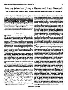
Figure 1: Segmented electrocardiograms (ECG) with adaptive constant and linear intervals (top) and non-adaptive piecewise linear (bottom). Only 150 data points out of 600 are shown. Both segmentations have the same model complexity, but we simultaneously reduced the fit and the leaveone-out cross-validation error with the adaptive model (top). Typically, in a time series segmentation, a single model is applied to all intervals. For example, all intervals are assumed to behave in a quasi-constant or quasi-linear manner. However, mixing different models and, in particular, constant and linear intervals can have two immediate benefits. Firstly, some applications need a qualitative description of each interval [48] indicated by change of model: is the tem-

perature rising, dropping or is it stable? In an ECG, we need to identify the flat interval between each cardiac pulses. Secondly, as we will show, it can reduce the fit error without increasing the cross-validation error. Intuitively, a piecewise model tells when the data is increasing, and at what rate, and vice versa. While most time series have clearly identifiable linear trends some of the time, this is not true over all time intervals. Therefore, the piecewise linear model locally overfits the data by computing meaningless slopes (see Fig. 1). Global overfitting has been addressed by limiting the number of regressors [46], but this carries the implicit assumption that time series are somewhat stationary [38]. Some frameworks [48] qualify the intervals where the slope is not significant as being “constant” while others look for constant intervals within upward or downward intervals [10]. Piecewise linear segmentation is ubiquitous and was one of the first applications of dynamic programming [7]. We argue that many applications can benefit from replacing it with a mixed model (piecewise linear and constant). When identifying constant intervals a posteriori from a piecewise linear model, we risk misidentifying some patterns including “stair cases” or “steps” (see Fig. 1). A contribution of this paper is experimental evidence that we reduce fit without sacrificing the cross-validation error or running time for a given model complexity by using adaptive algorithms where some intervals have a constant model whereas others have a linear model. The new heuristic we propose is neither more difficult to implement nor more expensive computationally. Our experiments include white noise and random walks as well as ECGs and stock market prices. We also compare against the dynamic programming (optimal) solution which we show can be computed in time O(n2 k). Performance-wise, common heuristics (piecewise linear or constant) have been reported to require quadratic time [27]. We want fast linear time algorithms. When the number of desired segments is small, top-down heuristics might be the only sensible option. We show that if we allow the one-time linear time computation of a buffer, adaptive (and non-adaptive) top-down heuristics run in linear time (O(n)). Data mining requires high scalability over very large data sets. Implementation issues, including numerical stability, must be considered. In this paper, we present algorithms that can process millions of data points in minutes, not hours. 2 Related Work Table 1 summarizes the various common heuristics and algorithms used to solve the segmentation problem with polynomial models while minimizing the Euclidean (l2 ) error. The top-down heuristics are described in section 7. When the number of data points n is much larger than the number of segments k (n ≫ k), the top-down heuristics is particularly competitive. Terzi and Tsaparas [42] achieved a

Table 1: Complexity of various segmentation algorithms using polynomial models with k segments and n data points, including the exact solution by dynamic programming. Algorithm Dynamic Programming Top-Down Bottom-Up Sliding Windows

Complexity O(n2 k) O(nk) O(n log n) [39] or O(n2 /k) [27] O(n) [39]

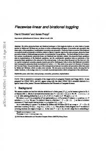
complexity of O(n4/3 k 5/3 ) for the piecewise constant model by running (n/k)2/3 dynamic programming routines and using weighted segmentations. The original dynamic programming solution proposed by Bellman [7] ran in time O(n3 k), and while it is known that a O(n2 k)-time implementation is possible for piecewise constant segmentation [42], we will show in this paper that the same reduced complexity applies for piecewise linear and mixed models segmentations as well. Except for Pednault who mixed linear and quadratic segments [40], we know of no other attempt to segment time series using polynomials of variable degrees in the data mining and knowledge discovery literature though there is related work in the spline and statistical literature [19, 35, 37] and machine learning literature [3, 5, 8]. The introduction of “flat” intervals in a segmentation model has been addressed previously in the context of quasi-monotonic segmentation [10] by identifying flat subintervals within increasing or decreasing intervals, but without concern for the cross-validation error. While we focus on segmentation, there are many methods available for fitting models to continuous variables, such as a regression, regression/decision trees, Neural Networks [25], Wavelets [14], Adaptive Multivariate Splines [19], Free-Knot Splines [35], Hybrid Adaptive Splines [37], etc. 3 Complexity Model Our complexity model is purposely simple. The model complexity of a segmentation is the sum of the number of regressors over each interval: a constant interval has a cost of 1, a linear interval a cost of 2 and so on. In other words, a linear interval is as complex as two constant intervals. Conceptually, regressors are real numbers whereas all other parameters describing the model only require a small number of bits. In our implementation, each regressor counted uses 64 bits (“double” data type in modern C or Java). There are two types of hidden parameters which we discard (see Fig. 2): the width or location of the intervals and the number

of regressors per interval. The number of regressors per interval is only a few bits and is not significant in all cases. The width of the intervals in number of data points can be represented using κ⌈log m⌉ bits where m is the maximum length of a interval and κ is the number of intervals: in the experimental cases we considered, ⌈log m⌉ ≤ 8 which is small compared to 64, the number of bits used to store each regressor counted. We should also consider that slopes typically need to be stored using more accuracy (bits) than constant values. This last consideration is not merely theoretical since a 32 bits implementation of our algorithms is possible for the piecewise constant model whereas, in practice, we require 64 bits for the piecewise linear model (see proposition 5.1 and discussion that follows). Experimentally, the piecewise linear model can significantly outperform (by ≈ 50%) the piecewise constant model in accuracy (see Fig. 11) and vice versa. For the rest of this paper, we take the fairness of our complexity model as an axiom.

c ax + b

m1

ax + b

m2

m3

4 Time Series, Segmentation Error and Leave-One-Out Time series are sequences of data points (x0 , y0 ), . . . , (xn−1 , yn−1 ) where the x values, the “time” values, are sorted: xi > xi−1 . In this paper, both the x and y values are real numbers. We define a segmentation as a sorted set of segmentation indexes z0 , . . . , zκ such that z0 = 0 and zκ = n. The segmentation points divide the time series into intervals S1 , . . . , Sκ defined by the segmentation indexes as Sj = {(xi , yi )|zj−1 ≤ i < zj } . Additionally, each interval S1 , . . . , Sκ has a model (constant, linear, upward monotonic, and so on). Pκ In this paper, the segmentation error is computed from j=1 Q(Sj ) where the function Q is the square of the l2 rePzj −1 (p(xr ) − gression error. Formally, Q(Sj ) = minp r=z j−1 yr )2 where the minimum is over the polynomials p of a given degree. For example, if the interval Sj is said to be constant, P then Q(Sj ) = zj ≤l≤zj+1 (yl − y¯)2 where y¯ is the average, P y¯ = zj−1 ≤l r > 2). Proof. We prove the result using the Euclidean (l2 ) norm, the proof is similar for higher order norms. We begin by showing that polynomial regression can be reduced PN −1 to ja matrix inversion problem. Given a polynomial Pq j=0 aj x , the square of the Euclidean error is i=p (yi − PN −1 j 2 j=0 aj xi ) . Setting the derivative with respect to al to zero for l = 0, . . . , N − 1,PgeneratesPa system of q N −1 j+l = N equations and N unknowns, i=p xi j=0 aj Pq l y x where l = 0, . . . , N − 1. On the right-handi=p i i Pq l side, we have a N dimensional vector (Vl = i=p yi xi ) whereas on the P left-hand-side, we have the N × N Tœplitz q i+l matrix Al,i = multiplied by the coefficients of i=p xi the polynomial (a0 , . . . , aN −1 ). That is, we have the matrixPN −1 vector equation i=0 Al,i ai = Vl . As long as N ≥ q − p, the matrix A is invertible. When N < q − p, the solution is given by setting N = q − p and letting ai = 0 for i > q − p. Overall, when N is bounded a priori by a small integer, no expensive numerical analysis is needed. Only computing the matrix A and the vector V is potentially expensive because they involve summations over a large number of terms. Once the coefficients a0 , . . . , aN −1 are known, we compute the fit error using the formula: q X i=p

 

N −1 X j=0

2

aj xji − yi 

=

N −1 N −1 X X

aj al

j=0 l=0

− 2

N −1 X j=0

aj

q X

xj+l i

i=p

q X i=p

xji yi +

q X

yi2 .

i=p

Again, only the summations are potentially expensive. Hence, computing the best polynomial fitting some data points over a specific range and computing the corresponding fit error in constant Pqtime is equivalent to computing range sums of the form i=p xii yil in constant time for 0 ≤ i, l ≤ 2N . To do so, simply compute once all prefix sums Pqj,l = Pq 5 Polynomial Fitting in Constant Time j l i=0 xi yi and then use their subtractions to compute range The naive fit error computation over a given interval takes queries Pq xj y l = P j,l − P j,l . q p−1 i=p i i linear time P O(n): solve 2for the polynomial p and then compute i (yi − p(xi )) . This has lead other authors Prefix sums speed up the computation of the range sums to conclude that top-down segmentation algorithm such as (making them constant time) at the expense of update time Douglas-Peucker’s require quadratic time [27] while we will and storage: if one of the data point changes, we may have to show they can run in linear time. To segment a time series recompute the entire prefix sum. More scalable algorithms

Table 2: Accuracy of the polynomial fitting in constant time using 32 bits and 64 bits floating point numbers respectively. We give the worse percentage of error over 1000 runs using uniformly distributed white noise (n = 200). The domain ranges from x = 0 to x = 199 and we compute the fit error over the interval [180, 185).

N = 1 (y = b) N = 2 (y = ax + b) N = 3 (y = ax2 + bx + c)

32 bits 7 × 10−3 % 5% 240%

64 bits 1 × 10−11 % 6 × 10−9 % 3 × 10−3 %

are possible if the time series are dynamic [31]. Computing the needed prefix sums is only done once in linear time and requires (N 2 + N + 1)n units of storage (6n units when N = 2). For most practical purposes, we argue that we will soon have infinite storage so that trading storage for speed is a good choice. It is also possible to use less storage [33]. When using floating point values, the prefix sum approach causes a loss in numerical accuracy which becomes significant if x or y values grow large and N > 2 (see Table 2). When N = 1 (constant polynomials), 32 bits floating point numbers are sufficient, but for N ≥ 2, 64 bits is required. In this paper, we are not interested in higher order polynomials and choosing N = 2 is sufficient. 6 Optimal Adaptive Segmentation

(see Algorithm 1). Once we have computed the r × n + 1 matrix, we reconstruct the optimal solution with a simple O(k) algorithm (see Algorithm 2) using matrices D and P storing respectively the best segmentation points and the best degrees. Algorithm 1 First part of dynamic programming algorithm for optimal adaptive segmentation of time series into intervals having degree 0, . . . , N − 1. 1: INPUT: Time Series (xi , yi ) of length n 2: INPUT: Model Complexity k and maximum degree N (N = 2 ⇒ constant and linear) 3: INPUT: Function E(p, q, d) computing fit error with poly. of degree d in range [xp , xq ) (constant time) 4: R, D, P ← k × n + 1 matrices (initialized at 0) 5: for r ∈ {0, . . . , k − 1} do 6: {r scans the rows of the matrices} 7: for q ∈ {0, . . . , n} do 8: {q scans the columns of the matrices} 9: Find a minimum of Rr−1−d,p +E(p, q, d) and store its value in Rr,q , and the corresponding d, p tuple in Dr,q , Pr,q for 0 ≤ d ≤ min(r + 1, N ) and 0 ≤ p ≤ q + 1 with the convention that R is ∞ on negative rows except for R−1,0 = 0. 10: RETURN cost matrix R, degree matrix D, segmentation points matrix P

Algorithm 2 Second part of dynamic programming algorithm for optimal adaptive segmentation. 1: INPUT: k × n + 1 matrices R, D, P from dynamic programming algo. 2: x ← n 3: s ← empty list 4: while r ≥ 0 do 5: p ← Pr,x 6: d ← Dr,x 7: r ←r−d+1 8: append interval from p to x having degree d to s 9: x←p 10: RETURN optimal segmentation s

An algorithm is optimal, if it can find a segmentation with minimal error given a model complexity k. Since we can compute best fit error in constant time for arbitrary polynomials, a dynamic programming algorithm computes the optimal adaptive segmentation in time O(n2 N k) where N is the upper bound on the polynomial degrees. Unfortunately, if N ≥ 2, this result does not hold in practice with 32 bits floating point numbers (see Table 2). We improve over the classical approach [7] because we allow the polynomial degree of each interval to vary. In the tradition of dynamic programming [30, pages 261–265], in a first stage, we compute the optimal cost matrix (R): Rr,p is the minimal segmentation cost of the time interval [x0 , xp ) using a model complexity of r. If E(p, q, d) is the fit error of a polynomial of degree d over the time interval [xp , xq ), 7 Piecewise Linear or Constant Top-Down Heuristics computable in time O(1) by proposition 5.1, then Computing optimal segmentations with dynamic programming is Ω(n2 ) which is not practical when the size of the Rr,q = min Rr−1−d,p + E(p, q, d) time series is large. Many efficient online approximate al0≤p≤q,0≤d5%), but more importantly, we reduce the leave-one-out crossvalidation error as well for small model complexities. As the model complexity increases, the adaptive model eventually has a slightly worse cross-validation error. Unlike for

13 Conclusion and Future Work We argue that if one requires a multimodel segmentation including flat and linear intervals, it is better to segment accordingly instead of post-processing a piecewise linear segmentation. Mixing drastically different interval models (monotonic and linear) and offering richer, more flexible segmentation models remains an important open problem. To ease comparisons accross different models, we propose a simple complexity model based on counting the number of regressors. As supporting evidence that mixed models are competitive, we consistently improved the accuracy by 5% and 13% respectively without increasing the crossvalidation error over white noise and random walk data. Moreover, whether we consider stock market prices of ECG data, for small model complexity, the adaptive top-down heuristic is noticeably better than the commonly used topdown linear heuristic. The adaptive segmentation heuristic is not significantly harder to implement nor slower than the top-down linear heuristic.

We proved that optimal adaptive time series segmentations can be computed in quadratic time, when the model complexity and the polynomial degree are small. However, Table 5: Comparison of top-down heuristics on ECG data despite this low complexity, optimal segmentation by dy(n = 200) for various model complexities: segmentation namic programming is not an option for real-world time series (see Fig. 4). With reason, some researchers go as far error and leave-one-out cross-validation error. as not even discussing dynamic programming as an alternative [27]. In turn, we have shown that adaptive top-down Fit error for k = 10, 20, 30. patient adaptive linear constant linear/adaptive heuristics can be implemented in linear time after the linear 100 99.0 110.0 116.2 111% time computation of a buffer. In our experiments, for a small 101 142.2 185.4 148.7 130% model complexity, the top-down heuristics are competitive 102 87.6 114.7 99.9 131% with the dynamic programming alternative which sometimes 103 215.5 300.3 252.0 139% offer small gains (10%). 104 124.8 153.1 170.2 123% Future work will investigate real-time processing for 105 178.5 252.1 195.3 141% online applications such as high frequency trading [48] and average 141.3 185.9 163.7 132% live patient monitoring. An “amnesic” approach should be 100 46.8 53.1 53.3 113% tested [39]. 101 55.0 65.3 69.6 119% 102 103 104 105 average 100 101 102 103 104 105 average patient 100 101 102 103 104 105 average 100 101 102 103 104 105 average 100 101 102 103 104 105 average

42.2 48.0 50.2 114% 88.1 94.4 131.3 107% 53.4 53.4 84.1 100% 52.4 61.7 97.4 118% 56.3 62.6 81.0 111% 33.5 34.6 34.8 103% 32.5 33.6 40.8 103% 30.0 32.4 35.3 108% 59.8 63.7 66.5 107% 29.9 30.3 48.0 101% 35.6 37.7 60.2 106% 36.9 38.7 47.6 105% Leave-one-out error for k = 10, 20, 30. adaptive linear constant linear/adaptive 3.2 3.3 3.7 103% 3.8 4.5 4.3 118% 4.0 4.1 3.5 102% 4.6 5.7 5.5 124% 4.3 4.1 4.3 95% 3.6 4.2 4.5 117% 3.9 4.3 4.3 110% 2.8 2.8 3.5 100% 3.3 3.3 3.6 100% 3.3 3.0 3.4 91% 2.9 3.1 4.7 107% 3.8 3.8 3.6 100% 2.4 2.5 3.6 104% 3.1 3.1 3.7 100% 2.8 2.2 3.3 79% 2.9 2.9 3.6 100% 3.3 2.9 3.3 88% 3.7 3.1 4.4 84% 3.2 3.2 3.5 100% 2.1 2.1 3.4 100% 3.0 2.7 3.6 90%

14 Acknowledgments The author wishes to thank Owen Kaser of UNB, Martin Brooks of NRC, and Will Fitzgerald of NASA Ames for their insightful comments. References [1] Yahoo! Finance. last accessed June, 2006. [2] S. Abiteboul, R. Agrawal, et al. The Lowell Database Research Self Assessment. Technical report, Microsoft, 2003. [3] D. M. Allen. The Relationship between Variable Selection and Data Agumentation and a Method for Prediction. Technometrics, 16(1):125–127, 1974. [4] S. Anand, W.-N. Chin, and S.-C. Khoo. Charting patterns on price history. In ICFP’01, pages 134–145, New York, NY, USA, 2001. ACM Press. [5] C. G. F. Atkeson, A. W. F. Moore, and S. F. Schaal. Locally Weighted Learning. Artificial Intelligence Review, 11(1):11– 73, 1997. [6] R. Balvers, Y. Wu, and E. Gilliland. Mean reversion across national stock markets and parametric contrarian investment strategies. Journal of Finance, 55:745–772, 2000. [7] R. Bellman and R. Roth. Curve fitting by segmented straight lines. J. Am. Stat. Assoc., 64:1079–1084, 1969. [8] M. Birattari, G. Bontempi, and H. Bersini. Lazy learning for modeling and control design. Int. J. of Control, 72:643–658, 1999. [9] H. J. Breaux. A modification of Efroymson’s technique for stepwise regression analysis. Commun. ACM, 11(8):556– 558, 1968. [10] M. Brooks, Y. Yan, and D. Lemire. Scale-based monotonicity analysis in qualitative modelling with flat segments. In IJCAI’05, 2005. [11] K. P. Burnham and D. R. Anderson. Multimodel inference: understanding aic and bic in model selection. In Amsterdam Workshop on Model Selection, 2004.

[12] S. Chardon, B. Vozel, and K. Chehdi. Parametric blur estimation using the generalized cross-validation. Multidimensional Syst. Signal Process., 10(4):395–414, 1999. [13] K. Chaudhuri and Y. Wu. Random walk versus breaking trend in stock prices: Evidence from emerging markets. Journal of Banking & Finance, 27:575–592, 2003. [14] D. L. Donoho and I. M. Johnstone. Ideal spatial adaptation by wavelet shrinkage. Biometrika, 81:425–455, 1994. [15] E. F. Fama and K. R. French. Permanent and temporary components of stock prices. Journal of Political Economy, 96:246–273, 1988. [16] W. Fitzgerald, D. Lemire, and M. Brooks. Quasi-monotonic segmentation of state variable behavior for reactive control. In AAAI’05, 2005. [17] D. P. Foster and E. I. George. The risk inflation criterion for multiple regression. Annals of Statistics, 22:1947–1975, 1994. [18] H. Friedl and E. Stampfer. Encyclopedia of Environmetrics, chapter Cross-Validation. Wiley, 2002. [19] J. Friedman. Multivariate adaptive regression splines. Annals of Statistics, 19:1–141, 1991. [20] T. Fu, F. Chung, R. Luk, and C. Ng. Financial Time Series Indexing Based on Low Resolution Clustering. ICDM-2004 Workshop on Temporal Data Mining, 2004. [21] D. G. Galati and M. A. Simaan. Automatic decomposition of time series into step, ramp, and impulse primitives. Pattern Recognition, 39(11):2166–2174, November 2006. [22] A. L. Goldberger, L. A. N. Amaral, et al. PhysioBank, PhysioToolkit, and PhysioNet. Circulation, 101(23):215– 220, 2000. [23] N. Haiminen and A. Gionis. Unimodal segmentation of sequences. In ICDM’04, 2004. [24] J. Han, W. Gong, and Y. Yin. Mining segment-wise periodic patterns in time-related databases. In KDD’98, 1998. [25] T. Hastie, R. Tibshirani, and J. Friedman. Elements of Statistical Learning: Data Mining, Inference and Prediction. Springer-Verlag, 2001. [26] J. Kamruzzaman, RA Sarker, and I. Ahmad. SVM based models for predicting foreign currency exchange rates. ICDM 2003, pages 557–560, 2003. [27] E. J. Keogh, S. Chu, D. Hart, and M. J. Pazzani. An online algorithm for segmenting time series. In ICDM’01, pages 289–296, Washington, DC, USA, 2001. IEEE Computer Society. [28] E. J. Keogh and S. F. Kasetty. On the Need for Time Series Data Mining Benchmarks: A Survey and Empirical Demonstration. Data Mining and Knowledge Discovery, 7(4):349–371, 2003. [29] E. J. Keogh and M. J. Pazzani. An enhanced representation of time series which allows fast and accurate classification, clustering and relevance feedback. In KDD’98, pages 239– 243, 1998. [30] J. Kleinberg and É. Tardos. Algorithm design. Pearson/Addison-Wesley, 2006. [31] D. Lemire. Wavelet-based relative prefix sum methods for range sum queries in data cubes. In CASCON 2002. IBM, October 2002.

[32] D. Lemire, M. Brooks, and Y. Yan. An optimal linear time algorithm for quasi-monotonic segmentation. In ICDM’05, 2005. [33] D. Lemire and O. Kaser. Hierarchical bin buffering: Online local moments for dynamic external memory arrays. submitted in February 2004. [34] D. Lemire, C. Pharand, et al. Wavelet time entropy, t wave morphology and myocardial ischemia. IEEE Transactions in Biomedical Engineering, 47(7), July 2000. [35] M. Lindstrom. Penalized estimation of free-knot splines. Journal of Computational and Graphical Statistics, 1999. [36] A. W. Lo and A. C. MacKinlay. Stock Market Prices Do Not Follow Random Walks: Evidence from a Simple Specification Test. The Review of Financial Studies, 1(1):41– 66, 1988. [37] Z. Luo and G. Wahba. Hybrid adaptive splines. Journal of the American Statistical Association, 1997. [38] G. Monari and G. Dreyfus. Local Overfitting Control via Leverages. Neural Comp., 14(6):1481–1506, 2002. [39] T. Palpanas, T. Vlachos, E. Keogh, D. Gunopulos, and W. Truppel. Online amnesic approximation of streaming time series. In ICDE 2004, 2004. [40] E. Pednault. Minimum length encoding and inductive inference. In G. Piatetsky-Shapiro and W. Frawley, editors, Knowledge Discovery in Databases. AAAI Press, 1991. [41] D. Sornette. Why Stock Markets Crash: Critical Events in Complex Financial Systems. Princeton University Press, 2002. [42] E. Terzi and P. Tsaparas. Efficient algorithms for sequence segmentation. In SDM’06, 2006. [43] I. Tomek. Two algorithms for piecewise linear continuous approximations of functions of one variable. IEEE Trans. on Computers, C-23:445–448, April 1974. [44] P. Tse and J. Liu. Mining Associated Implication Networks: Computational Intermarket Analysis. ICDM 2002, pages 689–692, 2002. [45] K.i Tsuda, G. Rätsch, S. Mika, and K.-R. Müller. Learning to predict the leave-one-out error. In NIPS*2000 Workshop: Cross-Validation, Bootstrap and Model Selection, 2000. [46] K. T. Vasko and H. T. T. Toivonen. Estimating the number of segments in time series data using permutation tests. In ICDM’02, 2002. [47] H. J. L. M. Vullings, M. H. G. Verhaegen, and H. B. Verbruggen. ECG segmentation using time-warping. In IDA’97, pages 275–285, London, UK, 1997. Springer-Verlag. [48] H. Wu, B. Salzberg, and D. Zhang. Online event-driven subsequence matching over financial data streams. In SIGMOD’04, pages 23–34, New York, NY, USA, 2004. ACM Press. [49] Y. Zhu and D. Shasha. Query by humming: a time series database approach. Proc. of SIGMOD, 2003.