Author’s Accepted Manuscript A bi-objective approach for scheduling groundhandling vehicles in airports Silvia Padrón, Daniel Guimarans, Juan José Ramos, Fitouri-Trabelsi Salma www.elsevier.com/locate/caor
PII: DOI: Reference:
S0305-0548(15)00296-8 http://dx.doi.org/10.1016/j.cor.2015.12.010 CAOR3901
To appear in: Computers and Operation Research Received date: 4 June 2013 Revised date: 26 June 2015 Accepted date: 17 December 2015 Cite this article as: Silvia Padrón, Daniel Guimarans, Juan José Ramos and Fitouri-Trabelsi Salma, A bi-objective approach for scheduling ground-handling vehicles in airports, Computers and Operation Research, http://dx.doi.org/10.1016/j.cor.2015.12.010 This is a PDF file of an unedited manuscript that has been accepted for publication. As a service to our customers we are providing this early version of the manuscript. The manuscript will undergo copyediting, typesetting, and review of the resulting galley proof before it is published in its final citable form. Please note that during the production process errors may be discovered which could affect the content, and all legal disclaimers that apply to the journal pertain.
A bi-objective approach for scheduling ground-handling vehicles in airports Silvia Padrón*1a, Daniel Guimarans1,2, Juan José Ramos1, Salma Fitouri-Trabelsi3 1
Dpt. Telecommunication and System Engineering, Universitat Autònoma de Barcelona, C/ Emprius, 2, 08202, Sabadell, Barcelona, Spain. e-mail:
[email protected] 2
Optimisation Research Group, National ICT Australia (NICTA), 13 Garden Street, Eveleigh NSW 2015, Australia. e-mail: {
[email protected]} 3
Mathématiques Appliquées, Informatique et Automatique pour l'Aérien (MAIAA) & Air Transportation Department, L'Ecole Nationale de l'Aviation Civile (ENAC), 7 Avenue Édouard Belin, 31055, Toulouse Cedex 04, France. e-mail: {
[email protected]} *
Corresponding Author: Tel +33 61198437 Present address: Industrial Organization, Logistics & Technology Department, Toulouse Business School, 20 Boulevard Lascrosses, 31068 Toulouse, France, e-mail:
[email protected],
[email protected] a
Abstract In the present paper, we propose a new approach for scheduling ground-handling vehicles, tackling the problem with a global perspective. Preparing an aircraft for its next flight requires a set of interrelated services involving different types of vehicles. Planning decisions concerning each resource affect the scheduling of the other activities and the performance of the other resources. Considering the different operations and vehicles instead of scheduling each resource in isolation allows integrating decisions and contributing to the optimization of the overall ground-handling process. This goal is defined through two objectives: (i) minimizing the waiting time before an operation starts and the total reduction of corresponding time windows and (ii) minimizing the total completion time of the turnarounds. We combine different technologies and techniques to solve the problem efficiently. A new method to address this biobjective optimization problem is also proposed. The approach has been tested using real data from two Spanish airports, thereby obtaining different solutions that represent a trade-off between both objectives. Experimental results permit inferring interesting criteria on how to optimize each resource, considering the effect on other operations. This outcome leads to more robust global solutions and to savings in resources utilization. Keywords: Air transportation, ground handling, multi-objective optimization, constraint programming, Vehicle Routing Problem with Time Windows 1. Introduction The notable growth of air traffic in recent years has led to increasingly congested airports and significant flights delays. In 2012, approximately 35% of European flights were more than 5 minutes late, with an average of 30 minutes [1]. A more collaborative coordination among all the involved actors, such as airports, airlines, air traffic management, ground handlers, etc., and a better planning of airport resources are crucial to improve the operational efficiency of the air transportation system. Different efforts and important projects are currently being carried out to achieve this goal, such as the Airport-Collaborative Decision Making (A-CDM) and the Single European Sky ATM Research (SESAR) programs [2,3], which is particularly focused on Air Traffic Management. Regarding turnaround, the TITAN Project [4] proposes to improve the efficiency of airport processes through sharing reliable and timely information among the concerned 1
actors. Turnaround is defined as the period of time the aircraft is on the ramp between an inbound and outbound flight, and different ground-handling operations are performed. Ground handling comprises the activities, operations procedures, equipment requirements, and personnel necessary to prepare an aircraft for the next flight. Many aircraft delays can be attributed to overlong turnarounds due to a lack of planning integration of the different activities and an inefficient use of resources [5]. In addition, the ground tasks are very interdependent. Each operation is a potential source of delays that could be easily propagated to other ground operations and other airport processes [6,7]. Divisions of either airports or airlines have historically performed these operations. With the recent process of deregulation of the ground-handling market at European airports, a notable increase in the number of third-party companies has taken place [8]. This new scenario, with several ground handlers providing multiple services, further increases the importance of efficient scheduling of ground activities [9]. Due to the hierarchy of overall airport planning, ground handlers are generally not included in the decision making of other scheduling processes (flight scheduling, stand allocation, etc.). This means they must fit their planning around a set of hard constraints. These constraints include aircraft arrival, departure, turnaround time, and stand allocation, among others [10]. Thus, ground handling appears an interesting and open field for research and technology transfer. In particular, logistics in ground handling [11] and cooperative planning decisions are among the major challenges to improving the quality of ground-handling services. In this context, the development of new tools that can help with the decision making process becomes mandatory. We present a novel and efficient bi-objective approach to tackling the groundhandling scheduling problem. To the best of our knowledge, this is the first time the problem is treated as a whole in the literature. Thus far, other approaches have been developed to optimize operations in isolation [9,12,13], but they do not consider the relationships and entanglements among all the involved activities. In our approach, we do explicitly consider such relationships and entanglements to solve the problem from a global perspective. To do so, we develop a biobjective optimization methodology and decompose the problem to apply efficient techniques. Thus, we first solve a planning problem that leads to multiple Vehicle Routing Problem with Time Windows (VRPTW) problems. These are solved individually, and decisions made on the routing are propagated to the other VRPTWs through reductions in the available time windows. This process provides a consistent method to solve the complete problem. Ground-handling procedures are usually divided into two types: terminal and ramp. Terminal activities are performed inside the terminal buildings and concern passenger services. Ramp operations take place at the aircraft parking position between the time it arrives at the stand (InBlocks) and its departure (Off-Blocks). Figure 1 shows an example of the principal activities during a typical turnaround when the aircraft is parked at a contact point (the stand is connected to the terminal via a bridge).
2
In-Blocks (IB)
Deboarding (DB)
Fueling (F)
Catering (Ca)
Cleaning (Cl)
Unloading Baggage (UL)
Potable water servicing (PW)
Loading Baggage (L)
Toilet Servicing (TS)
Boarding (B)
PushBack (PB)
Off-Blocks
Figure 1. Example of activity flow during a turnaround at a contact point Because the turnaround is a very complex process, its duration depends on many different variables. These include operational variables related to the aircraft type (size, number of seats), the number of tasks, parking position at a contact or remote stand, and the service time required to carry them out (full servicing or minimum servicing). Some activities are affected by precedence constraints imposed due to security issues, space requirements or airline policy; e.g., fueling cannot be performed simultaneously with deboarding/boarding. In some cases, the precedence constraints can be violated; e.g., fueling and deboarding can be performed simultaneously when a fire extinguisher is available. For hygienic reasons, the toilet and potable water servicing (collect the waste and re-equip with fresh water) cannot be performed at the same time, but either of the two can be performed first. The catering and cleaning processes usually must be finished before boarding starts and, sometimes, they can begin only when deboarding ends. The end of the turnaround process is determined by the Off-Block Time (OBT), when all doors are closed, the bridge is removed, the pushback vehicle is present and the aircraft is ready for startup and push back [6]. Although this operation might not be necessary for aircraft parked at a remote position, pushing away the aircraft (pushback) is the most typical method used for leaving the parking position. For that reason, we have defined pushback as the last task of the ground-handling service in our problem. Each operation is performed by a specific type of vehicle; therefore, different ground units or vehicles are necessary. According to the task, some vehicles with a given capacity must transport some quantity of resources to the aircraft stand (catering, fueling, or potable water operations) or collect waste from the aircraft (also catering, lavatory services or cleaning tasks). Likewise, some vehicles do not transport any resource (pushback, baggage loader or the fuel dispenser by underground pipelines). To simplify the model according to the goal of this work, we made some assumptions about the turnaround operations. We selected the main activities of a full servicing turnaround on aircraft parking at a contact point. In addition, we have not considered baggage transportation. Baggage transportation has special features in relation to other ground-handling activities; i.e., more than one trip is needed to carry all of the bags, more than one baggage facility can be used, etcetera. It requires a specific model and solution method and is an important field for future research.
3
At each aircraft, the operations must be performed within the defined turnaround time. Hence, a time window to begin the service is assigned to each activity that considers the duration of each task and the precedence constraints. Ground-handling vehicles must visit the stand where the aircraft is parked in the given time window, perform the operations during a determined service time, and travel to the next stands to perform their next activities. Scheduling decisions made for one service affect other activities. Tasks belonging to the same aircraft are related according to the precedence restrictions, as well as to their corresponding time windows. The time when an operation begins thus could reduce the time windows of the other activities, depending on these restrictions, and consequently the performance of the vehicles servicing them. Optimizing each resource while considering the effect on other operations permits an integration of planning decisions and contributes to optimizing the overall ground service process. For instance, scheduling the vehicles to complete the tasks as closely as possible to the start of their time window leaves some room to address unexpected events or delays. This is conductive to a more robust global solution, that is, while the operations begin at their corresponding original time windows, a reschedule is avoided. Solving this problem consists of obtaining a schedule for the ground-handling vehicles that service the aircraft performing turnaround during one working day. The schedule must satisfy temporal, precedence, and capacity constraints. We aim to minimize the operation waiting time, i.e., accomplishing each operation as early as possible in relation to its original time window, minimizing the total reduction of the time windows and considering the vehicles’ utilization. This leads to a second objective: to minimize the total completion time of the ground services at each aircraft. That is, we want to balance robustness of scheduling each operation with good performance of the turnaround, using the vehicles efficiently. In addition, we focus on solving the problem at a tactical level. This means that vehicles are scheduled using estimated flight arrival and departures times, predicted duration of operations and a planned gate assignment. In this sense, we are concerned with developing a flexible algorithm that can obtain good solutions with a reasonable computational effort. Operational planning and resource allocation in ground-handling companies are conditioned by prior mid-term decisions, usually made one month ahead, and by external changes on the day of operation. In the mid-term planning, ground handlers work based on flight schedules, aircraft types to be serviced and, perhaps, expected airport resources. Using this information, the handling equipment is allocated according to the planned workload. This quite often leads to an inefficient use of resources and being in an uncomfortable position to address unexpected events. By employing an optimization process as in the proposed approach, ground handlers can improve the utilization of their equipment while reducing costs. Moreover, we aim with this approach to increase the robustness of the operational plan for the equipment allocated in the mid-term planning. Robust solutions are crucial on the operation day to performing the turnaround within very tight time windows. Short delays caused by late start of a turnaround, perturbations during operations or ground-handler underperformance can be absorbed. Otherwise, departure delays can be produced, which turn into economic penalties. Different activities and type of vehicles, each of them with their own available fleet, are then considered to study the ground-handling problem from a global perspective. Scheduling these vehicles to perform the services at different aircraft could be modeled as a VRPTW [14]. The ground-handling problem is separated using a decomposition schema inspired by the workcenter-based decomposition for Job Shop Scheduling [15], and one VRPTW is identified for each type of vehicle. The well-known Insertion Heuristics method [16] and a hybrid methodology [17] were used to solve each VRPTW sub-problem. In this methodology, Constraint Programming (CP) was combined with Large Neighborhood Search (LNS) and Variable Neighborhood Descent (VND). To address the bi-objective problem, a new method we call Sequence Iterative Method (SIM) has been developed. Modifying the order in which the
4
sub-problems are solved yields a range of solutions representing the best compromise between the two objectives. The remainder of this article is organized as follows. In Section 2, the previous work related to vehicle scheduling in ground handling, the VRPTW and multi-objective optimization are reviewed. The decomposition approach used and the problem formulation are described in Section 3. Then, the proposed solution method and the method to address the bi-objective problem is presented in Section 4. Next, computational results are presented and discussed in Section 5. Finally, conclusions and future research lines are provided in Section 6. 2. Previous Studies 2.1 Ground-handling vehicle scheduling Vehicle scheduling in the ground-handling process has received less attention than other airport resources; few works can be found in the literature. Moreover, most of the examples found are focused on one type of resource. To the best of our knowledge, none of these works examine the scheduling of ground-handling vehicles as a whole. Regarding ramp operations, Du et al. [12] proposed a model to schedule fueling vehicles based on the Vehicle Routing Problem with Tight Time Windows (VRPTTW) with multiple objectives. They considered minimization of the number of vehicles, the start time of the service, and the total servicing time of the trucks, following this order of importance. An improved Ant Colony algorithm is presented to address the multi-objective problem. Clausen [9] focused on connecting baggage transportation and proposed a greedy algorithm based on an Integer Programming model for the Vehicle Routing Problem with Time Windows (VRPTW). Norin et al. [7] proposed an interesting integration of a simulation model of various operations during turnaround and the scheduling of de-icing trucks obtained by a greedy optimization algorithm. Minimizing the delays as well as the traveling time of the trucks are the objectives defined. A more sophisticated solution was proposed by Ho & Leung [13] to tackle airline catering operations including staff workload. They presented a comparison between Tabu Search and Simulated Annealing approaches to solve the problem. 2.2 VRPTW and the Multi-objective problem The Vehicle Routing Problem (VRP) is one of the most popular combinatorial optimization problems. It is aimed at determining an optimal set of routes for an available fleet of vehicles to service a set of customers, subject to different constraints. The VRPTW is an extension of the VRP in which each customer has a time window within which the vehicle must begin its task. The VRPTW has been extensively studied, and several formulations and exact algorithms have been proposed [18]. Solving this combinatorial optimization problem is NP-hard [19]; the use of heuristic algorithms [20], metaheuristics [21] and, recently, hybridization methods [22] has been a very important field of research. Many real-world optimization problems, including the VRPTW, involve more than one objective to be either minimized or maximized. The field of multi-objective optimization is drawing growing interest among researchers, particularly in VRPTW problems. To minimize the number of vehicles and the traveling distance, Gambardella et al. [23] implemented one of the more used methods: establishing a hierarchy between the objectives. In [12], a similar approach is used to solve a multi-objective model for scheduling fueling vehicles. Tan et al. [24] made a direct interpretation of the multi-objective problem using the concept of Pareto Optimality [25] in a hybrid multi-objective evolutionary algorithm (HMOEA), as did Ombuki et al. [26] with a genetic algorithm. A goal-programming model is proposed by Ghoseiri & Farid [27] in which the aspirations levels to the objectives and theirs deviations are minimized. Liu et al. [28] proposed a multi-objective heuristic in three phases to balance the workload, delivery 5
time and traveling distance among the vehicles. Hong & Park [29] also used a goalprogramming model to minimize total vehicle travel time and total customer waiting time. In a soft time window context, Müller [30] used the ε-constraint method to minimize the total cost and the penalties associated with violations of the time windows. Here, one of the objective functions is optimized and the other is converted into a constraint. For further examples and algorithms, an overview of the research in this area is presented in [31]. Usually, there is not a single solution optimizing all objectives simultaneously. Instead, different solutions can be found with a trade-off among the different objectives. The concept of domination or Pareto Optimality is used to determine this set of optimal solutions. It is said that a solution x dominates another y if and only if x is better than y in at least one objective and not worse in the other ones. That is, a solution is Pareto optimal if there is no other one that improves at least one objective function without sacrificing the others. Therefore, the obtained set of non-dominated points determines the Pareto optimal solutions of the multi-objective problem. A more formal definition of multi-objective problems and dominance is presented in [25]. Methods to address Multi-Objective Problems (MOP) can be classified according to the role of the decision maker in the decision process [32]. The more common classes are a priori, a posteriori, and interactive methods. The a priori approach uses specific information about the relevance of the objectives and user preferences before the solution process. As a result, one solution is found according to these preferences. In the a posteriori schema, a set of Pareto optimal solutions is generated and the preference information of each objective is used to select the most satisfactory one. Finally, in the interactive methods, the preference information is updated during the solution process. Different examples of methods classified as described above can be found in the literature, each having strengths and weaknesses. A good summary is presented in [32,33]. The advantage of the a priori approach is that it can produce a single compromise solution without requiring further participation of the decision maker. One of the methods more widely used due to its simplicity is the weighted method. Specifically, it is used in the mentioned de-icing trucks scheduling [7]. It involves aggregating all the objectives into one composite function with different weights that are used to indicate the relative importance among the criteria. However, there are problems in which expressing the preferences through values or correlate different objectives in the same function could yield inaccurate solutions [32,34]. In our particular case, tackling the vehicle-scheduling problem as a bi-objective problem contributes to the global approach of the ground-handling problem, although it is not easy to define the relationships and the importance among the objectives. The first criterion addresses the VRPTW problem for minimizing the total customer waiting time. However, this leads to more vehicles being involved. Although minimizing the number of vehicles is not an explicit optimization objective, it should be considered to solve the problem. Having waiting time on the preceding operation does not always imply that successive operations could not be started at the earliest point of their time windows. For instance, let there be two tasks with different durations, which must be finished before a third one. The task with the shorter service time will end earlier, but the third operation might need to wait for the second task anyway. Hence, it is possible to use the vehicles more efficiently, allowing waiting time on the first activity without affecting the completion time of the overall performance. The second objective is focused on the turnaround process. It is important to perform each operation as early as possible to minimize the completion time of the turnaround. On the other hand, minimizing the completion time leads to a reduction of the time windows of the operations on the same aircraft and thus increases the number of vehicles needed. For that reason, obtaining a set of solutions with a trade-off between the objectives yields the possibility of selecting the one that better suits the problem.
6
3. Problem Decomposition and Formulation The decomposition schema used in this work is inspired by the workcenter-based decomposition for the Job Shop scheduling problem [15]. A workcenter is a group of machines performing similar operations. In this approach, the overall problem is broken down into workcenter-based sub-problems, and they are solved independently. The operations of a subproblem are related to other sub-problem operations by the precedence restrictions. Each time a sub-problem is scheduled, new constraints for the other operations are generated. Therefore, a method that integrates the sub-solutions and keeps the consistency of the overall solution is needed. In our problem, each type of vehicle can be viewed as a workcenter, and the vehicles available in the fleet as the machines. Additionally, each task must be performed by just one type of vehicle. Therefore, instead of solving a global VRPTW, it is possible to solve local VRPTWs for each type of vehicle. In addition, scheduling each type of vehicle separately permits the development of specific methods to tackle special features according to the operation they perform. On the other hand, the temporal restrictions on performing each operation due to the defined turnaround time and the precedence constraints must be tackled globally. This ensures that the local solutions can be integrated to obtain a complete solution. The decomposition schema is shown in Figure 2. A procedure we called Temporal Constraints Level Procedure (TCLP) was defined to satisfy the temporal restrictions. For each type of vehicle, a VRPTW is modeled using the defined Routing Level Procedure (RLP). F1 and F2 are the defined optimization objectives. Global Problem
F2
TCLP
Sub-problems
RLP1
RLP2
...
f 11
f 12
...
RLPn
f1i f 1n F 1 i N
Figure 2. The problem decomposition schema The main features of this algorithm are modeled and implemented in Constraint Programming (CP). CP is a very attractive paradigm due to its expressiveness for modeling problems with side constraints. It has received much attention in recent decades due to its potential for solving real-world combinatorial optimization problems [35]. These applications often involve a heterogeneous set of side constraints and, typically, they must address frequent update/addition of constraints [36]. The flexibility of CP is thus a powerful characteristic because adding constraints is a modeling issue and does not affect the search process. In CP, problems are expressed by means of three elements: variables, their corresponding domains, and the constraints relating these variables. Solving a problem involves the assignment of values to the variables that satisfy all the constraints. This class of problems is usually termed Constraint Satisfaction Problems (CSP), and the core mechanism used in solving them is constraint propagation [37]. It involves deleting from variable domains values that cannot satisfy the problem constraints. When a value is assigned to a variable, it is propagated through the associated constraints to the rest of the variables involved in these constraints. If there are values 7
in other variable domains that are incompatible with propagated assignments, they are also removed [36]. Through constraint propagation, unfeasible alternatives are eliminated in advance, reducing the exploration of the search space. The parameters of the ground-handling problem are described as follow. Let Τ= {1,...,t} be the set of tasks to be carried out on the aircraft at its parking position. N= {1,..., n} is the set of scheduled aircraft performing a turnaround, and Α is the set of aircraft types. Each task i Τ according to aircraft type a Α has a duration δia, a requirement for goods ρia, and precedence restriction rules Ψia, which represent the set of tasks that must be finished before task i can start on aircraft type a. Each task must be performed by one type of vehicle. The set of types of vehicle is described by VT and each vt VT has its own homogeneous fleet Mvt ={1..mvt} with capacity Qvt. For each aircraft j N, the STAj and STDj are the scheduled arrival and departure times, respectively. The aircraft type is aj Α, and γj Γ is the stand where the aircraft is parked during the turnaround. Γ is the set of parking positions, and πij ∀i, j Γ, the traveling cost between stands and between them and the vehicle depot π0,i. There are O= T N operations to be performed by the vehicles from VT. An operation oij is a task i Τ performed at an aircraft j N according to aj A, the aircraft type of j. 3.1 Temporal Constraint Level Procedure (TCLP) In this level, the earliest and latest start times for each operation are obtained. Let the variable τij be the start time of each operation oij with a discretized initial domain τ:: [STAj..STDj]. The precedence restrictions are described by the following constraint: ij i' j i' a j i ,i' ,| i' ia j ,j N
(1)
Equation (1) ensures that temporal relationships among the tasks are fulfilled according to the type of aircraft to which they belong. When this restriction is propagated, the domain of the start time variable of each operation is reduced such that: τij:: [estij..lstij], where est and lst are the lower and upper bounds of τ and represent the operation’s earliest and latest start time, respectively. During the operation scheduling process, these time windows are modified due to the precedence restrictions. Note that the duration of the last operation, i.e., pushback, is not included. As mentioned, the end of the turnaround is defined as the start time of the pushback. Because the vehicles are routed separately, an explicit update process of the time windows is required to avoid inconsistency among sub-problems. Suppose two operations on the same aircraft, o11 and o 21 such that o11 must be finished before o 21 could start, that is, 21 11 1a . The difference between est11 and est21 is the duration of o11 , as well as between lst11 and lst21 . Suppose also that the type of vehicle which performs o11 is routed first and o11 is scheduled such that 11 est11 . The value of est21 is now 11 1a . Then, the time window of o 21 must be reduced. Otherwise, when the type of vehicle associated with o 21 is routed with the original time window, an infeasible solution might be obtained. Note that both the earliest and the latest start time could be reduced. For example, if o 21 is solved first, the lst11 will be 21 1a . The strategy followed to update the time windows and ensure the consistency of the solutions is further explained in Section 4. 3.2 Routing Level Procedure (RLP) When the time windows for each operation are calculated, a sub-problem is identified for each vtVT. We obtain the set of operations to be performed by each vt, Ovt={o1,..,on}, as well as the 8
duration do and the requirements for goods ro for each oOvt according to the task and the aircraft type where the operation takes place. Because each routing problem is solved separately and to simplify the notation, we identify set Ovt as O ={1,..,n}. The CP model corresponding to each VRPTW sub-problem is based on the formulation presented in [38]. Let V= O F L be the set of visits to be performed where set O= {1,..,n} represents the operations, i.e., the aircraft to be serviced. Two special visits describe the depot from which the vehicles start and finish their routes and are modeled by sets F= {n+1,..,n+m} and L= {n+m+1,…,n+2m}, respectively. m is the number of vehicles needed for all the operations to be accomplished by fleet M= {1…m}. Note that m is a parameter in our model. The visits fk= n+k, fkF and lk= n+m+k, lkL, represent the first and last visit of the vehicle kM, respectively. The following variables are defined: vi ∀i V: the vehicle which perform each visit i with domain v :: [1..m] pi ∀i V–F: the direct predecessor of a visit i with domain p :: [1..n+m] si ∀i V –L: the direct successor of a visit i with domain s :: [1..n,n+m+1..n+2m] ti ∀i V: the time when the visit i is performed with domain t :: [esti..lsti]. Notice the est and lst values are those obtained from the TCLP procedure qi ∀i V: the cumulated capacity after each visit i with domain q :: [0..Q] As mentioned, one of the optimization goals is accomplishing the operations as early as possible. Therefore, the objective function aims at minimizing the total difference between the earliest possible time a vehicle could perform each visit and the corresponding earliest service time. Let wi=ti-esti be this difference, that is, the client waiting time. The routing problem is then formulated as follows:
min wi
(2)
iN
Subject to vi v pi
i V F
(3)
vi v si
i V L
(4)
v fk vlk
k M
(5)
pi p j
i , j V F i j
s pi i i V F
(6) (7) (8)
p si i i V L
(9)
si s j
i , j V L i j
t i t pi pii d pi
ti t si isi d si
i V L
i V F
(10) (11)
qi q pi ri
i V F
(12)
qi q si rsi
i V L
(13)
Constraints (3) and (4) ensure a visit, its predecessor and successor, are assigned to the same vehicle, as well as the first and last visit of this vehicle with constraint (5). Inequalities (6) and (7) restrict a visit to have one and only one predecessor and successor, whereas constraints (8) and (9) keep the coherence between the successor and predecessor. To ensure the temporal precedence in a route, constraints (10) and (11) specify that the time to visit a client is at least (at most) the time to visit its predecessor (successor) plus (minus) the sum of traveling time and the duration of the service. Constraints (12) and (13) were defined to address the capacity restrictions of the vehicles. The goods picked up or delivered in the route are counted to keep the load along the route. 9
3.3 Decomposition bi-objective problem To obtain a more robust scheduling, the operations should be performed as early as possible within their original time windows. Because of the decomposition, the operation waiting time is calculated by the RLP with the updated time window (if it is reduced). If the size of the time window becomes smaller, most likely the waiting time would also be smaller, although it does not contribute to the solution robustness. Additionally, this reduction could lead to an increase in the vehicles needed. Therefore, our first objective aims at performing operations as soon as possible through two arguments: minimizing the total operation waiting time and the total reduction of the time windows. Let ∆i=(oesti-esti)+(olsti-lsti), where oesti and olsti mean the original values of the time windows obtained from the TCLP, i.e., the very earliest and latest start times for each operation. wi is the client waiting time set in Section 3.2. An aggregate function f1 is defined to describe how early the operations are performed in each routing problem: f 1vt i wi vt VT
(14)
iN
The first objective F1 is defined as: min f1vt vtVT
(15)
Let l be the last operation on each aircraft and τ the start time of operations defined in Section 3.1; the second objective F2 of this problem is:
min lj jN
(16)
The objective function F2 minimizes the completion time in all aircraft. 4. Solution Method In this section, we describe a new bi-objective algorithm developed for solving the groundhandling problem. This method is based on a workcenter-based decomposition strategy [15]. Most workcenter-based decomposition methods are derived from the Shifting Bottleneck procedure [15] developed by Adams et al. [39] and later improved by Balas et al. [40]. This decomposition heuristic was originally implemented for the classical job shop-scheduling problem and then extended to model other versions such as sequence-dependent times and workcenter problems, also called the parallel machine problem. At each round, a critical unscheduled sub-problem according to the optimization criterion is identified and solved as a one-machine (or workcenter) scheduling problem. Using this result, each sub-problem solved in the previous iterations is re-optimized by solving again a one-machine problem, whereas the machines already scheduled remain fixed. This re-optimizing cycle is repeated a number of times, modifying the order in which the machines are solved. The Shifting Bottleneck is computationally intensive and involves solving many single machine-scheduling problems [41]. Applying this procedure in our particular case, where each sub-problem is a VRPTW, can lead to long execution times; the problem becomes impractical to solve. Thus, we followed a similar schema but combined two processes to obtain a complete solution at each iteration. In the first process, which we call Solving Process, all sub-problems are solved one after another given a predefined order. Each time a sub-problem is solved, the time windows of the remaining sub-problems are updated to maintain consistency among the sub-solutions. The Solving Process is embedded in an iterative schema that we call Sequence Iterative Method (SIM). The goal of this second process is to improve the overall solution when dealing with the defined bi-objective optimization problem. The sequence for solving the sub-
10
problems is modified at each iteration according to the solution obtained, and the Solving Process is repeated with the new sequence. 4.1 Solving Process In the Solving Process, sub-problems are identified and solved according to a given sequence. A schema of this process is shown in Figure 3. First, the TCLP implemented using CP is used to find the time windows of each operation. Then, a sub-problem is identified for each type of vehicle and a routing problem is solved by means of the RLP. Solving sequence
Obtain the initial time windows
TCLP
Identify all the sub-problems Update the time windows N Select sub-problem
Are all the subproblems solved?
Exit Y
Routing a subproblem Find an initial solution
Make a local search process RLP
Figure 3. Flow diagram for the Solving Process The RLP procedure was developed in two stages. At the first stage, a well-known route construction heuristic is used to obtain a reasonably good initial solution (see Section 4.2). The number of vehicles obtained in this step is taken as an upper bound of the vehicles needed to perform the operations. Imposing this value as the size of the available fleet, a CP local search process is applied in the second stage to improve the initial solution. With this heuristic, we assume that there are sufficient resources to handle the airport workload. The CP methodology is described in Section 4.3. The aim of this step is to improve the initial solution by minimizing the operation waiting time, f1. After solving a sub-problem, an explicit process to update the time windows is needed to ensure consistency with the rest of the sub-problems, as explained in Section 3.1. Once again, taking advantage of the propagation of CP through the TCLP, a simple strategy is applied to maintain consistency. Finally, when all sub-problems are solved, the process is stopped. Algorithm 1 describes the proposed Solving Process. 1. Set SF 2. Obtain the initial time windows by means of TCLP 3. Sub-problems solution by means of the RLP 3.1 Repeat until |SF|=|VT| a. Choose siS b. Obtain an initial solution for si using the I3 Insertion Heuristic c. Apply the CP-based local search process d. Set SF SF {si} e. Update the time windows of the sub-problems in S\SF by means of the TCLP
Algorithm 1. Solving Process 11
Let S be the set of routing sub-problems to be solved, where |S|=|VT| and SF is the set of subproblems already solved SF S. To ensure coherence among sub-solutions, each time a subproblem is solved, the scheduled decisions are propagated to the rest of the sub-problems not yet solved, keeping the already-scheduled sub-problems fixed. First, no sub-problem has been solved. The very earliest and latest start time of each operation is obtained by means of the TCLP. When a sub-problem is scheduled, the start times of the operations belonging to this subproblem are calculated. Afterwards, the TCLP is recalled with the start times of the subproblems already solved. These values are propagated to the operations of the unscheduled subproblems, and their time windows are updated. This process is repeated for each sub-problem, always keeping the preceding scheduling decisions. Infeasible intermediate solutions are avoided using this strategy. Note that time window reductions depend on the order in which sub-problems are solved and affect the quality of the global solution. In fact, in the decomposition procedures based on Shifting Bottleneck, determining the next machine to be scheduled is one of the more important steps. According to [15], the sequence in which the machines are included in the partial schedule can reduce the re-optimization process without loss in solution quality. Then, the proposed iterative process (see Section 4.4) is developed, aiming at improving the solution by modifying the order in which sub-problems are solved. 4.2 Initial solution The initial solution of each routing problem is obtained using the Insertion Heuristic method [16]. Solomon proposed three variants (I1, I2 and I3), each using a different criterion to select customers to be inserted in a route. Moreover, a set of parameters was defined that permits adjusting the solution method to solve different problems. In particular, we used the third heuristic (I3). It is known [16, 20] that I1 yields the best results, particularly for traveling distance, which is a critical decision rule in this case. Nevertheless, in our problem, we aim to minimize the operation waiting time without compromising the number of vehicles required. Hence, the route construction should be guided by both geographical and time criteria with similar importance. In I3, the combination of the additional distance and time required to visit a customer is used to decide the best insertion place and the client to be inserted. Note that in this case, I1 and I3 are equivalent using the following parameters: (λ=0) for I1 and (α3 =0) for I3. However, a third parameter is included in I3 to assign priority to a client having the lowest deadline to begin the service. Among other aspects, this parameter contributes to reducing the vehicle waiting time which, in turn, can lead to reducing the number of vehicles required. Thus, we have decided that I3 is the most appropriate heuristic to obtain an initial solution for our problem. 4.3 Local search process A hybrid methodology based on [17] was selected to improve the initial solution found with I3. In this methodology, the modeling and the constraint propagation advantages of CP were combined with local search methods. Using the concept of operators based on Large Neighborhood Search (LNS) [42], the local search process is embedded in CP. These operators destroy and repair the solution to re-optimize parts of the problem. Destroy in this case means identifying a set of customers to remove from a solution. Repair refers to finding a better method to reinsert these customers into the partial solution. In addition, the methodology employs Variable Neighborhood Search (VNS) as a metaheuristic to guide the search. VNS was introduced by Hansen and Mladenovic [44] and has been applied to solve different variants of the VRP with interesting results [21,43,45,46]. Specifically, the Variable Neighborhood Descent (VND) [47] method has been adopted. A generic representation of this methodology is depicted in Figure 4.
12
Employing LNS within VND permits systematic exploration of the search space. Using VND, the algorithm moves from one operator to the next to escape from local minima. Any time an improved solution is found, the process is reset to the first operator; otherwise, the algorithm changes to the next operator. Initial solution x Define kmax operators k ←1 N Exit
k ≤ kmax Y
Destroy xp←dk(x) Operator Ok (LNS)
Repair x'←rk(xp)
N If f(x') ≤ f(x) Y x ←x' k ←1
k ←k+1
Figure 4 Flow diagram of the VND schema using LNS operators Two operators have been used for solving our problem: the Random Pivot OPerator (RPOP) [17] and the SMAll RouTing (SMART) [43]. According to Rousseau et al. [43], the neighborhood structure defined by used operators should be different to succeed with the VND. In RPOP, individual customers are removed and re-inserted, whereas SMART works with arc exchanges. In RPOP, the destroy method consists of randomly selecting a pivot customer, which is removed from the solution. Then, a set of the nearest customers according to their geographic proximity is also removed, forming a hole around the pivot [17]. Two key aspects should be considered when implementing the destroy methods in operators: (i) how to select customers, and (ii) how many, i.e., the size of the neighborhood. Concerning the first point, a typical strategy is removing clients that are related according to some criteria, i.e., geographic proximity. As for the second consideration, small neighborhoods are usually preferred to large ones due to computational time limitations. In our particular problem, different operations (clients) can have the same parking position due to the length of the schedule time horizon. Hence, establishing temporal criteria seems more suitable to remove visits than using geographical rules. In the ground-handling problem, the time windows to accomplish the operations are generally tight, particularly when the activities have precedence restrictions. Therefore, we have defined the closeness of the time windows as the proximity metric of the RPOP. Regarding the number of clients, the RPOP operator is defined such that the number of visits removed is gradually increased each time the search becomes trapped in a local minimum. One single pivot is again selected when an improvement is found. An upper limit on the number of pivots is defined to avoid exploring too-large neighborhoods. In the SMART operator, sequences of arcs in different routes are removed instead of customers. First, a random primary pivot is identified and a certain number of clients after and before the pivot are disconnected, making a hole in its route. Then, a set of secondary pivots is selected, 13
that is, the one customer in each other route that can be visited in that hole while making a minimal detour. The same process is applied several times, and a number of precedent and successive customers are removed. A CP-based Branch and Bound (BB) procedure is employed as the repairing method in the RPOP operator. Constraint propagation provides efficiency to this pruning of the search tree each time the upper bound is updated when a better solution is found. Additionally, the combination of VND and LNS plays an important role because different neighborhoods can be explored and revisited iteratively with improved upper bounds [17]. Because this process is exact, a limited execution time is established to avoid excessive computational time. In the case of the SMART, Limited Discrepancy Search (LDS) is used in the CP-BB procedure for repairing the solution as suggested Rousseau et al. [43]. The SMART operator is more likely to produce large neighborhoods than is the RPOP. With LDS, large search spaces can be explored more quickly without notably compromising the quality of the solution. 4.4 Sequence Iterative Method (SIM) As explained in Section 2.2, we define the ground-handling problem as a Multi-objective Optimization Problem (MOP), in particular, as a bi-criteria optimization problem. The first criterion relates to the quality of the local routing decisions and depends on the contraction of the time windows during the process. The second criterion can be observed as a global objective: minimizing the completion time of turnarounds. The iterative process was implemented to re-optimize the global solution due to the decomposition regarding the two defined objectives. Using a posteriori methods, the solution of the MOP is the set of non-dominated solutions, also called the Pareto optimal set. Depending on the problem, obtaining all Pareto optimal solutions is not guaranteed or can take high computational times [32,49]. Heuristic approaches, local search methods, metaheuristics, and evolutionary algorithms find approximations to the Pareto optimal set [50]. A definition of this approximation is also presented in the mentioned work: a solution y obtained by an algorithm A is Pareto optimal relative to A if A does not find another solution z such that z dominates y. In general, heuristic methods must be developed with two important principles: (i) find non-dominated points as close as possible to the optimal set and (ii) find solutions sufficiently diverse to provide a good coverage of this set [50]. Many methods such as the weighted method, ε-constraint, and goal programming among others solve the MOP by scalarization [31,32,49], i.e., transforming the problem into a single objective or a set of single objective problems. This strategy employs efficient and already tested singleobjective algorithms existing in the literature and applies them to solve the MOP. With the goals of more directly addressing the MOP and of finding a set of non-dominated points, these basic scalars, usually a priori methods, can be used as a posteriori approaches modifying the parameters. The ε-constraint procedure is commonly used with this approach. The problem is solved with respect to one objective and, at each iteration, the value of the second objective obtained is used as a constraint to limit the search space [30,32,49]. Following this scalarization schema, we developed SIM to find the potential non-dominated solutions for our problem. The problem is solved with respect to the first objective, and the value of the second objective is calculated from the obtained solution. At each round, the sequence for solving the sub-problems is modified to find a solution in the Pareto set to cover it in the best possible way. Regardless of the type of aircraft, the ground-handling service always finishes by pushing away the aircraft from its parking position (pushback). We used this information to create an initial sequence to obtain a lower bound of F2. The sub-problems are ordered and solved such that a promising search space will be explored to improve F1 while a new value for the second objective is obtained. This method is described in Algorithm 2.
14
Definition S: set of sub-problems where |S|=|VT|, slo: last operation, BL: sub-problems to solve before slo SR: remainder of the sub-problems, SSol: set of solutions found, 1 SSol 2 SR sort SR by the values that were assigned to identify the sub-problems Step A. Initial solution 3 4 5
Initial sequence to obtain a lower bound of F2 BL S {slo} SR SolvingProcess(S) Sequence to improve F1 keeping the position of slo
6 7 8 9 10 11 12 13 14 15 16 17 18
repeat SR' sort SR by f1vt in a decreasing order S' {slo} SR' SolvingProcess(S') if (F1'