A bio-inspired algorithm for location search in peer to peer network

Contents

A bio-inspired location search algorithm for peer to peer networks Sachin Kulkarni, Niloy Ganguly, Geoffrey Canright, Andreas Deutsch . . .

1

List of Contributors

Sachin Kulkarni Department of Computer Science and Engineering, Indian Institute of Technology Kharagpur, India, 721302 [email protected]

Geoffrey Canright R&D Telenor, Oslo, Norway [email protected]

Niloy Ganguly Department of Computer Science and Engineering, Indian Institute of Technology Kharagpur, India, 721302 [email protected]

Andreas Deutsch Center for Information Services and High Performance Computing (ZIH), TU-Dresden, Dresden 01062 [email protected]

A bio-inspired location search algorithm for peer to peer networks Sachin Kulkarni1 , Niloy Ganguly1 , Geoffrey Canright2 , and Andreas Deutsch3 1

2 3

Department of Computer Science and Engineering, Indian Institute of Technology Kharagpur, India [email protected],[email protected] R&I Telenor, Oslo, Norway [email protected] Center for Information Services and High Performance Computing (ZIH), TU-Dresden, Dresden 01062 [email protected]

Abstract In this paper, we propose a new p2p network based location search algorithm. The algorithm is built upon the concept of a gradient search and is applicable to unstructured networks. It is inspired by a biological phenomenon called haptotaxis. The algorithm performs much better than the random walk algorithm and is also more efficient than flooding. We also present some mathematical reasoning to explain the superiority of the algorithm.

1 Introduction A p2p based system is a network that relies on the computing resources available from all the participants in the network instead of concentrating on a small number of centralized servers. This kind of network allows to build a server-less infrastructure, where participating nodes cooperate to find the desired resources. Moreover many p2p architectures offer inherent scalability and robustness as the network reorganizes itself in case of dynamic entry and removal of nodes. However there is a cost associated with these desirable properties. The latency of locating the desired resource in the network increases as we use a p2p network. Optimizing this lookup time is one of the primary challenges of p2p systems. In this chapter, we propose a new algorithm based on a gradient search, which is a key-based algorithm. It performs a guided search for a desired key in the entire search space. The algorithm is motivated by a biological phenomenon called haptotaxis, hence named “hapto-search” [2]. We have previously developed algorithms for search, which are inspired by the natural immune system

2

Sachin Kulkarni, Niloy Ganguly, Geoffrey Canright, and Andreas Deutsch

and chemotaxis [4], [5]. Both haptotaxis and chemotaxis are used in biological interacting cell systems to regulate cell migration [3]. The regulated cell migration phenomenon inspires us to build a gradient-based search algorithm.

2 Related work Based on the type of neighborhood relationship between the nodes, p2p systems can be classified as structured and unstructured/semistructured. For unstructured p2p networks, one of the simplest approach is flooding, which is adopted by Gnutella [9]. Although flooding quickly finds out the desired location, it is inefficient as it produces a huge number of message packets. [1] describes random walk strategies in power law networks. It shows that kwalker random walk is much more scalable search method than flooding but at the expense slight increase in the average number of hops. It also discusses replication-based search strategies and its analysis shows that the search cost expected in such strategies is nr ,where n is the network size and r is the number of replicas. Our algorithm, hapto-search is also a replication-based algorithm. However we observed that the hapto-search algorithm is far more time efficient. Our algorithm to some extent resembles the algorithm used in loosely structured p2p systems such as freenet [10]. In structured p2p systems, the network topology is tightly controlled and the placement of the resources is done not at random nodes but at specific locations. This helps the queries to locate the desired resources efficiently. The highly structured p2p systems like CHORD and CAN use precise placement algorithms to achieve performance bound of log N , where N is the number of nodes in the network. However the imposition of the structure on the topology restricts their ability to operate in presence of extremely unreliable nodes. In hapto-search, we assume totally unstructured network, hence is extremely robust.

3 Definition of the hapto-search algorithm In this section, we discuss the hapto-search algorithm, its inspiration and details of how it works. 3.1 Design goal and basic idea Main design goal of this algorithm is to attain a speed of location search comparable to DHTs (i.e. log(N )) but to make no assumption about the structure of the network. Structured networks are more prone to failure and incur overhead to achieve robustness while robustness is a natural property of unstructured networks.

A bio-inspired location search algorithm for peer to peer networks

3

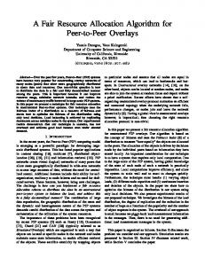
The algorithm defines a gradient-based search, in which every node is assigned a k-bit key unique within our p2p network. The key represents the identity of the node (Node ID, IP Address). A node distributes its key to a fixed number of peers in the network at random. When a peer wants to search for a node, it tries to search for any node, which has the key of the destination. To do so, a query traverses in the network and the next destination of the query is chosen in such a way that it ensures that the query always moves “closer” to the destination than the current position.

j j1 j2

h a a1 a2

h1 h2 h3

a3 a4

h4

j3 j4 g g1 g2 g3

i i1 i2 i3

b b1 b2 b3

g4 f

i4

f1 f2 f3

b4 d

c c1 c2 c3 c4=kx

f4

e d1 d2 d3 d4=kx

e1 e2 e3 e4

Fig. 1. Sketch of a network showing how the hapto-search algorithm operates. Each node is hosting 4 keys received from random peers. This diagram illustrates a case where node g wants to find node x (Node x is not shown in the figure). Nodes c and d have the key of x. Node g forwards the query to a neighbor, which has a key closer to kx (node h in this case). This way a query traverses in the network and ultimately reaches node c. The path indicated by arrows shows a possible query traversal.

3.2 Our inspiration - haptotaxis Migration of cells within our body is a fundamental process for example in tissue development, tumor metastasis or wound healing. To achieve appropriate physiological outcomes, cells must adjust direction and speed of their movement in response to environmental stimuli. There are cell adhesion proteins

4

Sachin Kulkarni, Niloy Ganguly, Geoffrey Canright, and Andreas Deutsch

at the outer surface of the cells, which bind to the adhesion ligands present in the extracellular matrix (ECM). This extracellular matrix is a substratum that surrounds the cells in a tissue. Cells tend to move in the direction where the adhesion between ECM ligands and cell receptors is larger. It is believed that the magnitude of this adhesion influences cell speed and random turning behavior, whereas a gradient of adhesion affects the resultant direction of cell movement. This phenomenon of a guided and gradient based movement of cells is called haptotaxis. Haptotaxis is influenced by the presence of the ECM consisting of immobilized molecules. Alternatively, cell migration towards a gradient of diffusible and soluble substances is known as chemotaxis. In our example, the ECM resembles a p2p network. Then, a query path in the p2p network can be viewed as a haptotactic cell movement in the ECM. Accordingly, the concept of haptotaxis gives an idea of a guided search towards the destination so that one can always make sure that at every step, the moving entity is getting “closer” to its destination. 3.3 Detailed algorithm In this section, we introduce the detailed algorithm, which is key-based. It allows nodes to retrieve location information of each other. The key assigned to each node is unique across the network. This key can be generated by hashing the user id into a n-bit length code. Every node distributes its key, location information (IP Address) to a fixed number of nodes in the network. This distribution is done at random. A node (say) A knows the location information of another node (say) B, if it has the key of B. Thus if one node wants to search the location information of the destination, it tries to search for any node, which has the key for this destination. Once it finds such node, it can get the desired location information from it. If a node doesn’t have the key required, it routes the query to the neighbor, which is closest to the destination. A neighbor is said to be closer to the destination if it has a key which is closer to the destination key (in terms of Hamming distance) than the current node. The closest neighbor is selected to forward the query. This way the algorithm ensures that the query always moves “closer” to the destination as the Hamming distance between destination key and the closest key present at the current node always decreases, or in the worst case remains the same. The search ends when the query reaches a node hosting the destination key (i.e. Hamming distance becomes zero). Figure 1 illustrates the steps of the algorithm. We have developed two versions of this algorithm, simple and restricted. In the simple version, the next hop to forward the query is chosen regardless of whether it has already been visited during the same search query or not. As it doesn’t remember the path, it may happen that a query goes into the loop and keeps on moving in the circular path because of its deterministic nature. In the case of the restricted version, we maintain the path vector storing all the nodes visited during the search in that order. The query is forwarded to such

A bio-inspired location search algorithm for peer to peer networks

5

a neighbor which is closer to the destination and which has not already been visited during the search. Thus loops are avoided and the query is guaranteed to reach the destination within N hops. Algorithm: Hapto-search input : Key of the destination node output: Location information of destination node current ←source ; while current node doesn’t have the destination key do for all the neighbors of current node in the network do shortest ← GetShortestHammingDistance (neighbor,destination); if neighbor’s shortest distance < my shortest distance then Add the neighbor to the sorted list of prospects end if neighbor’s shortest distance > farthest then Store neighbor and neighbor’s distance as farthest end end while List of prospects is not empty do node ← take a node from the sorted list with minimum distance; /* In the restricted version, this if condition is necessary whereas in the simple version, no such check is performed. */ if node not already visited in the search process then current ← node; break; end end if no such node available then /* This is the condition of dead end */ current ← choose the neighbor with the largest distance end end

Algorithm 1: Searching a key in an unstructured peer to peer network using the hapto-search algorithm. The input to the algorithm is the key for the destination and the output is the location information of the destination. The diagram shows both the simple and the restricted version of the algorithm. In the simple version, query is forwarded to a neighbor with shortest possible distance (and shorter than the current node’s shortest distance) where as in the restricted version, besides choosing shortest of the shortest, a path vector is maintained to store all the nodes visited during the search and query is forwarded to a neighbor only if it is not present in the path vector.

6

Sachin Kulkarni, Niloy Ganguly, Geoffrey Canright, and Andreas Deutsch Algorithm: Random search input : Key of the destination node output: Location information of destination node current ←source ; while current node doesn’t have the destination key do node ← Choose a node at random from the list of neighbors of current node current ← node end

Algorithm 2: Searching a key in an unstructured peer to peer network using the random-search algorithm. In this algorithm, next hop is chosen at random from the list of neighbors. Dead end: It may happen that the current node itself is closer to the destination than all its neighbors. We can call this a dead end as there is no closer neighbor to forward the query. In such case, we continue the search by sending the query to the farthest neighbor, i.e. the node for which the Hamming distance of its key from the destination key is largest among all the neighbors of the current node. The occurrence of dead ends implies the presence of local maxima in the search space. Dead ends will slow down the speed of the search algorithm. However, occurrence of dead ends depends upon the number of times a key is replicated as well as the average network degree. The details of both the simple and the restricted version of the hapto-search algorithm are illustrated through algorithm 1 whereas algorithm 2 depicts the simple random-search algorithm in which, the next hop to forward the query is chosen at random among the list of neighbors of the current node. The random-search algorithm is used as a benchmark to measure the efficiency of the hapto-search algorithm.

4 Analysis of hapto-search In this section, we present analysis of the hapto-search algorithm. We will be considering the simplified version of the algorithm for the analysis and the underlying network is assumed to be an E-R graph. We will be mainly interested in finding an upper bound for the average number of hops. 4.1 Average number of hops Consider an E-R graph of N nodes with average node degree M . Now in our algorithm, every node distributes its key to say, R peers at random such that every peer has approximately R keys. Without loss of generality, we can assume the key of the destination to be 0 (all n bits are zero). In the simple

A bio-inspired location search algorithm for peer to peer networks

7

hapto-search algorithm, a node not having the destination key, forwards the query to a neighbor which is “closer” to the destination or at least as close as the current node. To compute the average number of hops, we need to derive formula for the rate of change in Hamming Distance (∆HD) per hop traversal of the query. We need to know the probabilities of the current node being a local maximum and a global maximum. This can be represented by Plm and Pgm respectively. We also need to introduce two more parameters, Average Forward Move (AFM) and Average Backward Move (ABM), where AFM is defined as the average change in HD of the current node from the destination in a single hop if the current node is not a maximum. Similarly ABM is defined as the average change in HD of the current node from the destination in a single hop if the current node is a local maximum. Using these parameters, we can calculate ∆HD as the following theorem states. Theorem 1. In the simple hapto-search algorithm, the expected change in HD (∆HD) in a single hop traversal of query is given as: ∆HD = Plm ∗ (−ABM ) + (1 − Plm − Pgm ) ∗ AF M Proof: Consider a scenario where the current node is at HD i from the destination (destination key is assumed to be 0). Now there are three cases. 1. If the node is a global maximum (a node having the replication of destination key): In this case, search algorithm ends. So ∆HD = 0 2. If the node is a local maximum (dead end): In this case, it forwards the query to the farthest possible neighbor. Here HD is increased by the value ABM . So ∆HD = ABM 3. Otherwise: The current node finds a neighbor closer to the destination than itself to forward the query. In this case, HD is reduced by the value AF M . So ∆HD = AF M Therefore we can say that, ∆HD = Plm ∗ (−ABM ) + (1 − Plm − Pgm ) ∗ AF M The average number of hops can be directly calculated from ∆HD. The following theorem states that. Theorem 2. Given that ∆HD is the expected change in HD in a single traversal of the query and IHD is the HD of the source (query generating) node from the destination, average number of hops taken by the query to reach the destination is given by the equation: Hops =

IHD ∆HD

Now we will derive a formula for the probability of a local maximum, AF M and ABM .

8

Sachin Kulkarni, Niloy Ganguly, Geoffrey Canright, and Andreas Deutsch

4.2 Probability of a local maximum A local maximum is a node, which doesn’t have the destination key and it has no neighbor, which has a key closer to the destination key than the best key available at the node itself. Without loss of generality we can assume that the destination key is 0. In such case, there will be n Ci nodes in the network, which may have their key at HD i from the destination, where n is the number of bits used to define the key of a node. So the number of possible keys at HD i from the destination (h(i)) can be given as, h(i) = n Ci

(1)

Let H(i) denote the number of keys at HD > i from the destination. Then H(i) can be computed by the following equation n X

H(i) =

(h(k))

(2)

k=i+1

To compute the probability of a local maximum, let us first derive the formula for the probability that a node is at HD i from the destination. Theorem 3. Given the destination key as 0, the probability that a node is at HD i from the destination is given by: Pi =

R X

h(i)

(

j=1

Cj ∗ H(i) CR−j ) 2n C R

Proof: A node will be at HD i from the destination if it has at least one key which is at HD i from the destination and no other key is closer than i. Each node has R keys in its storage. So there are R ways of it, where in each case the current node has j keys at HD i (1 ≤ j ≤ R). So the total number of ways a node can have at least one key at HD i can be given as, ni =

R X

(h(i) Cj ∗ H(i) CR−j )

j=1

Now the total sample set consists of the number of ways of choosing R keys n from all possible keys. Total number of possible keys is 2n . So there are 2 CR ways of choosing R keys for a node. Hence the probability that a node at HD i can be given as, R h(i) X Cj ∗ H(i) CR−j ( Pi = ) 2n C R j=1 Theorem 4. The probability that a node is a maximum is given as, P =

n−1 X

n X

h=0

j=h+1

(Ph ∗ (

Pj )M )

A bio-inspired location search algorithm for peer to peer networks

9

Proof: The probability of a maximum is the probability that the best key available at the current node has HD less than the best key available at any of its neighbors. This can happen in many ways. A node can have best key at HD 0 (P0 ) and keys available at all its M neighbors are at HD 1..n (n is the number of bits in a key). The probability of this case can be given P as (P0 ∗ ( nj=1 Pj )M ). Alternatively, a node can have the best key at HD 1 and all the keys available at its neighbors are at HD 2..n and so on. Hence the probability of a maximum is summation of probabilities of all such cases. Hence P can be given as, P =

n−1 X

n X

h=0

j=h+1

(Ph ∗ (

Pj )M )

This equation gives us the probability of a maximum in the network, which includes both global and local maximum. When the query reaches a node at a global maximum, the search algorithm ends. As there are R replications of R . every key in the network, probability of a global maximum Pgm will be N Hence the probability of a local maximum will be Plm = P − Pgm . 4.3 Average forward move (AFM) In order to compute the AFM, let us define P bi , which denotes the probability that the best possible neighbor of the current node is at HD i from the destination, given that the current node is not a maximum. Theorem 5. The probability that the best possible neighbor of the current node is at HD i from the destination given that current node is not a maximum, is, P bi = (1 −

i−1 X

Pk )M − (1 −

k=0

i X

Pk )M

k=0

Proof: That the best possible neighbor of the current node is at HD i indicates that all the neighbors are at HD ≥ i with at least one neighbor at HD i. We know that the probability of a node being at HD i is i . Then the probability PP i−1 of all M neighbors being at HD ≥ i will be (1 − k=0 Pk )M . But this also includes the case where all the neighbors arePat HD > i with no neighbor at i HD i. This can occur with probability (1 − k=0 Pk )M . We need to exclude this probability from the answer. Hence P bi can be given as, P bi = (1 −

i−1 X

Pk )M − (1 −

k=0

i X

Pk )M

k=0

Theorem 6. The expected value of an average forward move (AFM) is given by the equation: AF M =

n X

(hd ∗

hd=1

n X i=hd

(Pi ∗ P bi−hd ))

10

Sachin Kulkarni, Niloy Ganguly, Geoffrey Canright, and Andreas Deutsch

Proof: When a node is not a maximum, it has a neighbor which can reduce the HD further by value between 0 and n. We call this reduction in HD as ∆HD. Then the AFM can be computed as, n X

AF M =

(hd ∗ P (∆HD = hd))

hd=1

Consider a case when the best neighbor reduces the HD by 1 (i.e. ∆HD = 1). This is possible when the current node is at HD 1 and the best neighbor is at HD 0 or the current node is at 2 and the best neighbor is at HD 1 and so on. So the probability of ∆HD = 1 is, P (∆HD = 1) =

n X

(Pi ∗ P bi−1 )

i=1

In general we can say that the probability of ∆HD = hd is, P (∆HD = hd) =

n X

(Pi ∗ P bi−hd )

i=hd

Substituting value of P (∆HD = hd) in AFM formula, we can say that n X

AF M =

(hd ∗ P (∆HD = hd))

hd=1

4.4 Average backward move (ABM) In order to compute ABM, let us define P fi+hd , which denotes the probability that the farthest possible neighbor of the current node is at HD i from the destination, given that the current node is a maximum. Theorem 7. The probability that the farthest possible neighbor of current node is at HD i + hd from the destination, given that the current node is a maximum and at HD i is, P fi+hd = (

i+hd X

i+hd−1 X

Pk )M − (

Pk )M

k=i+1

k=i+1

Proof: This proof is quite similar to the proof of theorem 5. Theorem 8. The expected value of the average backward move (ABM) is given by the equation: ABM =

n X

(hd ∗

hd=1

n−hd X

(Pi ∗ P fi+hd ))

i=1

Proof: This proof is quite similar to the proof of theorem 6. We performed various experiments to verify all these formulae. Details of these experiments will be discussed later in the performance evaluation section.

A bio-inspired location search algorithm for peer to peer networks

11

4.5 Analysis of random search In the case of random search, a node chooses the neighbor to forward the query at random and when the query reaches the node having the destination key replica, the algorithm ends. We can derive a formula for the expected number of hops for the random search. A similar formula has been derived in [1]. We are presenting the result for the completeness of the article. Theorem 9. Let R be the number of replications of the key of a node in the network and N be the number of nodes in the network. Then the expected number of hops taken by the random search is given as Hopsran =

∞ X R R ∗ ( (i ∗ (1 − )i )) N N i=0

Proof: Let Pran (i) be the probability that the destination key replica is found at the ith hop. Then Hopsran can be given as, Hopsran =

∞ X (i ∗ Pran (i)) i=0

Given the key replication value R and the network size N , the probability R that a node has the destination key replica is N . Now probability that the R R )∗ N as it is query finds the destination key replica in one hop is (1 − N the case when first node doesn’t have the destination key (probability of this R R )) and the second one has it (probability being N ). Similarly being (1 − N the probability that the query finds the destination key replica in two hops is R R 2 ) ∗N . In general case, we can say that the probability of finding the (1 − N destination key at ith hop (Pran (i)) is, Pran (i) = (1 −

R i R ) ∗ N N

Substituting this into the formula of Hopsran , we get Hopsran =

∞ X R R ∗ ( (i ∗ (1 − )i )) N N i=0

5 Performance evaluation This section presents the results of the performance evaluation of the haptosearch algorithm. The experimental setup as well as the specific experiments which are performed to evaluate the performance are noted next.

12

Sachin Kulkarni, Niloy Ganguly, Geoffrey Canright, and Andreas Deutsch

5.1 Experimental setup We ran the algorithm (both simple and restricted versions) on E-R networks. For each network, and for different values of key replication, we ran the algorithm for randomly chosen 2000 source-destination pairs. The key size is considered as 32 for all the cases. We were mainly interested in the following aspects: 1. Experimental verification of the theoretical prediction made for the simple version of the hapto-search algorithm 2. Performance analysis of the restricted version. The performance is measured in terms of the average number of hops. We compared the performance of the restricted version of the algorithm with state-of-the-art algorithm: • the random search in unstructured p2p networks • DHT-based search in structured p2p networks 3. Understanding the dependence of the performance parameters upon the network size N for the restricted version of the algorithm. 5.2 Simple version - Experimental results and their prediction by theoretical analysis We ran the simple version of the hapto-search on E-R networks with different values of N (number of nodes) and R (key replication). We measured the values of AFM, ABM, average hops and the number of dead ends. The number of dead ends are computed by a method called Steepest Ascent Graph (SAG) 4 . Figure 2 shows the comparison between theoretical and experimental values of the parameters, AFM, ABM and the probability of a local maximum. It can be seen that for all the plots, theoretical and experimental values match. Figure 3 shows the same comparison for the average number of hops. Here we observe that the average number of hops (both experimentally and theoretically) in the case of the simple version is insensitive to the changes in the key replication value. One can also observe that there is a slight difference between the theoretical and experimental values for this plot. This is due to the practicalities of the implementation of the simple version. As no path vector is maintained, the query tends to go in a loop most of the times. To avoid this, a TTL (Time To Live) value is used to restrict the number of hops. The search is considered as a failure if the query doesn’t reach the destination within TTL hops. We haven’t considered the failure cases during the plot. It was experimentally observed that only 5-10% of the queries turn out to be successful. The successful queries are the lucky queries, which find the 4

Steepest Ascent Graph (SAG): SAG is constructed for a given network, destination and the key distribution. Every node maintains only a link with the best neighbor and drops the rest of the links. All the nodes having a self-loop are maxima.

A bio-inspired location search algorithm for peer to peer networks 10

10

Theoretical value of AFM Experimental value of AFM

Theoretical value of ABM Experimental value of ABM

9

ABM (Average Backward Move)

AFM (Average Forward Move)

9

8

7

6

5

4

3

2

8

7

6

5

4

3

2

1

1

0 10

13

20

30

40

50

60

70

R (Key Replication Value)

80

90

0 10

100

20

30

40

50

60

70

80

90

R (Key Replication Value)

The probability of a local maximum

0.1

Theoretical value of probability Experimental value of probability

0.09

0.08

0.07

0.06

0.05

0.04

0.03

0.02

0.01

0

0

20

40

60

80

100

120

140

R (Key Replication Value)

Fig. 2. Comparison of theoretical and experimental values of the parameters, Average Forward Move (AFM), Average Backward Move (ABM) and the probability of a local maximum (Plm ). The first figure shows AFM on the y-axis vs key replication value on the x-axis for the E-R network of 10K nodes, M=10. The second figure shows the plot of ABM on the y-axis vs key replication value on the x-axis where as the third figure plots the probability of local maxima for the same configuration. As one can observe, the theoretical and the experimental values match for all these parameters. Also interesting to note is that the parameter values except in the initial phase are almost independent of the replication value R.

100

14

Sachin Kulkarni, Niloy Ganguly, Geoffrey Canright, and Andreas Deutsch 20

Theoretical value of hops Experimental value of hops

The average number of hops

18

16

14

12

10

8

6

4

2

0

0

10

20

30

40

50

60

70

80

90

100

R (Key Replication Value)

Fig. 3. Comparison of theoretical and experimental values of the average number of hops. The figure depicts the plot of the probability of a local maximum on the y-axis vs key replication value on the x-axis for the E-R network of 10K nodes, M=10. As one can observe, there is a slight mismatch between the theoretical and the experimental values. The average number of hops is largely insensitive to the key replication value.

destination in a shorter path. Hence the experimental values of the average number of hops tend to be smaller than the theoretical values. In the next section, we analyze the performance of the restricted version of the hapto-search, which can also be considered as a more practical version. 5.3 Performance of the restricted version In this section we compare the performance of the restricted hapto-search with the random search algorithm and DHT-based search algorithm. Moreover, the experimental testing of the scalability of the algorithm is reported. Comparison with random search Figure 4 shows the comparative plot of the average number of hops needed for the random search and the hapto-search algorithm for an E-R network with 10000 number of nodes and average degree 10. One can see that the hapto-search algorithm performs far better than random search. The average number of hops taken by the random search algorithm at key replication value 140 is 276.6 whereas for the hapto-search algorithm even at the key replication value of 10, the number of average hops needed is 98.4. This shows that the gradient-based guided search is far more efficient than the random search. Comparison with DHT and scalability analysis We know that the performance bound on DHT-based search algorithms is log N . Therefore we tried to compare the performance of the hapto-search

A bio-inspired location search algorithm for peer to peer networks

15

2500

Hapto−search on network with N=10K, M=10 Random search on network with N=10K, M=10

Average Number of Hops

2000

1500

1000

500

0

20

40

60

80

100

120

140

R (Key Replication Value)

Fig. 4. Comparative plot of the average number of hops on the y-axis vs key replication value on the x-axis for the random search and the hapto-search algorithm on an ER network with N=10000 and average degree (M)=10. 8

350

Key Replication=30 log(N)

Key Replication=20 Key Replication=30 Key Replication=40 Key Replication=50 Key Replication=60 0.0055*N

300

7

Average Number of Hops

log(H) (H: Average Number of Hops)

7.5

6.5

6

5.5

5

250

200

150

100

4.5 50 4

3.5 12

12.5

13

13.5

14

14.5

15

log(N) (N: Number of nodes in the network)

15.5

16

0

0

1

2

3

4

5

N (Number of nodes in the network)

Fig. 5. Plot of average number of hops vs the number of nodes (N ). The first figure is a log-log plot of the average number of hops (H) required to reach the destination with key replication value = 30 on the y-axis and the number of nodes on the x-axis. It also shows log-log plot of log N . It can be seen that the slope of the curve log N is much less than that of the average number of hops, which shows that hapto-search does not scale to log N . In the second plot, a E-R network of degree 10 is considered with different key replication values = 20, 30, 40, 50 and 60 respectively. It can be seen that the average number of hops varies linearly with N (number of nodes in the network) unlike the formula for the average hops for the simple version of the algorithm, which is independent of N . As the key replication value increases, the slope of the curve decreases.

6 4

x 10

16

Sachin Kulkarni, Niloy Ganguly, Geoffrey Canright, and Andreas Deutsch

with log N . The first plot in figure 5 shows this comparison. It is a log-log plot of the average number of hops vs the number of nodes in the network. log N is also plotted for the comparison. It can be seen that the performance of the hapto-search does not scale to log N . We then tried to evaluate the effect of the key replication on the average number of hops. The second plot in the figure 5 shows the average number of hops vs the network size for E-R networks of degree 10 and for different values of R (key replication value) ranging from 20 to 60. Previously we saw that the formula for the average number of hops for the simple version of the algorithm is not dependent upon the network size N . Moreover, we found that the performance is also largely insensitive to R. But in the restricted version, we see that the average number of hops increases linearly with N . Also the performance is dependent on R. As the value of R increases, the slope of the curve for the average number of hops decreases. We are still working towards formulating a theory behind the dependence upon N in the restricted version. As a first step, we have made some important observations regarding the behavior of the parameters, AFM and ABM in the restricted version. This is noted next. 6.2

ABM for the restricted version

ABM (Average Backward Move)

AFM (Average Forward Move)

AFM for the restricted version 3.4

3.2

3

2.8

2.6

2.4 0.5

1

1.5

2

2.5

3

3.5

4

N (Number of nodes in the network)

4.5

5

6

5.8

5.6

5.4

5.2

5 0.5

4

x 10

1

1.5

2

2.5

3

3.5

4

4.5

N (Number of nodes in the network)

Fig. 6. Plot of the parameters Average Forward Move (AFM) and Average Backward Move (ABM) vs the network size (N ). The first figure shows AFM on the y-axis vs N on the x-axis for the E-R network with key replication value 10, M=10 for the restricted version whereas the second figure plots ABM on the y-axis vs the network size N on the x-axis for the same configuration.

Dependence of AFM and ABM upon N Figure 6 shows the plot of AFM and ABM vs the network size N for the restricted version. The first figure shows the plot of AFM vs the network size N whereas the second figure shows the plot of ABM vs the network size N .

5 4

x 10

A bio-inspired location search algorithm for peer to peer networks

17

Here one can observe that the values of AFM and ABM increase linearly with N . The rate of change in AFM and ABM are different.

6 Conclusion and future work In this paper, we have discussed a new bio-inspired algorithm for location search in an unstructured peer to peer network. It is a key-based search algorithm, which ensures that the query always moves “closer” and ultimately reaches the destination. We demonstrated that the algorithm is far more efficient than plain random walk. We presented two versions of the algorithm, a simple version as well as a restricted version. A rigorous theoretical analysis to explain the simple version is reported. The theoretical predictions and the experimental results match to a high degree of precision. We observed that the performance parameters such as the average number of hops, the probability of a local maximum, AFM and ABM is independent of the network size N . While studying the experimental results of the restricted version, we identified that these performance parameters are also dependent on N . Hence we have realized that the theory proposed here needs to be suitably modified in the future to explain the experimental results of the restricted version of the hapto-search. Moreover, all the results presented here are from the experiments on the random networks. Future work will also explore other interesting and realistic topologies like the small-world and power law networks.

References 1. Q. Lv, P. Cao, E. Cohen, K. Li, and S. Shenker. Search and Replication in Unstructured Peer-to-peer Networks. In Proceedings of the 16th International Conference on Supercomputing, pages 84-95. ACM Press, 2002. 2. B. Alberts, A. Johnson, J. Lewis, M. Raff, K. Roberts, and P. Walter. Molecular Biology of the Cell, fourth edition, Garland Science, New York, 2002 3. A. Deutsch, and S. Dormann. Cellular Automaton Modeling of Biological Pattern Formation, Birkhauser, Boston, 2005 4. N. Ganguly, G. Canright, and A. Deutsch. Design of an Efficient Search Algorithm for p2p Networks Using the Concepts from Natural Immune Systems, In proceedings of PPSN VIII: The 8th International Conference on Parallel Problem Solving from Nature, 18-22 September 2004, Birmingham, UK. 5. G. Canright, A. Deutsch, and T. Urnes. Chemotaxis-Inspired Load Balancing, In the proceedings of the European Conference on Complex Systems, November 2005. 6. O. Babaoglu, G. Canright, A. Deutsch, G. Di Caro, F. Ducatelle, L. Gambardella, N. Ganguly, M. Jelasity,, R. Montemanni, A. Montresor. Design Patterns from Biology for Distributed Computing ACM Transaction of Autonomous and Adaptive Systems, Vol 1 Issue 1, September 2006. 7. T. Urnes. An Analysis of the Skype Peer-to-Peer Protocol Internal Publication, Telenor R&D, May 2006.

18

Sachin Kulkarni, Niloy Ganguly, Geoffrey Canright, and Andreas Deutsch

8. J. Rosenberg, J. Weinberger, C. Huitema and R. Mahy. STUN: Simple Traversal of User Datagram Protocol (UDP) Through Network Address Translators (NATs), RFC 3489, IETF, Mar. 2003. 9. http://www.gnutella.com 10. Open Source Community. The free network project - rewiring the internet. In http://freenet.sourceforge.net/, 2001.