In the Proceedings of the Asian Conference on Computer Vision (ACCV), 2010 ... framework for general parametric curves, we derive its differential prop- erties ...
In the Proceedings of the Asian Conference on Computer Vision (ACCV), 2010
A biologically-inspired theory for non-axiomatic parametric curve completion Guy Ben-Yosef and Ohad Ben-Shahar Computer Science Department , Ben-Gurion University , Beer-Sheva , Israel
Abstract. Visual curve completion is typically handled in an axiomatic fashion where the shape of the sought-after completed curve follows formal descriptions of desired, image-based perceptual properties (e.g, minimum curvature, roundedness, etc...). Unfortunately, however, these desired properties are still a matter of debate in the perceptual literature. Instead of the image plane, here we study the problem in the mathematical space R2 × S 1 that abstracts the cortical areas where curve completion occurs. In this space one can apply basic principles from which perceptual properties in the image plane are derived rather than imposed. In particular, we show how a “least action” principle in R2 ×S 1 entails many perceptual properties which have support in the perceptual curve completion literature. We formalize this principle in a variational framework for general parametric curves, we derive its differential properties, we present numerical solutions, and we show results on a variety of images.
1
Introduction
Although the visual field is often fragmented due to occlusion, our perceptual experience is one of whole and complete objects. This phenomenon of amodal completion, as well as its counterpart process of modal completion (where the object is illusory), are fundamental part of perceptual organization and visual processing [17], and they have been studied by all of the perceptual, neuropysiological, and computational vision communities. Inspired by this interdisciplinary nature of visual completion research, in this work we present a new and rigorous mathematical curve completion theory, which is motivated by neurophysiological findings and at the same time uses only basic principles to provide explanations and predictions for existing perceptual evidence. The problem of curve completion usually assumes that the completed curve is induced by two oriented line segments, also known as the inducers, and hence it is typically formulated as follows: Problem 1. Given the position and orientation of two inducers p0 = [x0 , y0 ; θ0 ] and p1 = [x1 , y1 ; θ1 ] in the image plane, find the shape of the “correct” curve that passes between these inducers. While “correctness” of the completion and hence the problem as a whole are ill defined, it is typical to aspire for completions that agree the most with perceptual and neurophysiological evidence, usually by the application of additional
2
Guy Ben-Yosef and Ohad Ben-Shahar
constraints. Unfortunately, however, while different constraints have been proposed, they were inspired more by intuition and mathematical elegance, and less by perceptual findings or neurophysiological principles. In the next section we first review some of the relevant computational models, the axiomatic approach which often motivates them, and the extent to which they agree with existing perceptual and neurophysiological evidence.
2
Previous work
Many computational curve completion studies, including Ullman’s [22] seminal work, employ an axiomatic perspective to the shape of the completed curve, i.e., they state the desired perceptual characteristics that the completed curve should satisfy. Among the most popular axioms suggested are – isotropy - invariance of the completed curve to rigid transformations. – smoothness - The completed curve is analytic (or in some cases, differentiable once). – total minimum curvature - integral of curvature along the curve should be as small as possible. – extensibility - any two arbitrary tangent inducers along a completed curve C should generate the same shape as the shape of the portion of C connecting them. – Scale invariance - the completed shape should be independent on the viewing distance. – Roundedness - the shape of a completed curve induced by two cocircular inducers should be a circle. – Total minimum change of curvature - integral of the derivative of curvature along the curve should be as small as possible. Evidently, some of the suggested perceptual axioms conflict each other, and hence much debate exist in the computational literature as to which axioms are the “right” ones, a choice which affects the entailed completion model. Among the first suggested models, the biarc model, was proposed by Ullman [22], who sought to satisfy the first four axioms from the list above. According to this model, the completed curve between two inducers consists of two circular arcs, each tangent both to an inducer and to the other arc. Since the number of such biarc pairs is infinite, the axiom of minimal total curvature helps to narrow down the possible completions to one unique curve. While Ullman took the axiom of total minimum curvature in the narrow scope of biarc curves only, the same axiom was studied in its strict sense by Horn [9], and later Mumford [15]. The resulting class of curves, known as elastica, R minimizes the functional that expresses total curvature square k(s)2 ds, and its corresponding Euler-Lagrange equation leads to a differential equation that must be solved in order to derive the elastica curve of two given inducers. An arclength parametrization form of this equation was shown to be 1 θ˙2 = sin(θ + φ), c
(1)
A biologically-inspired theory for non-axiomatic parametric curve completion
3
where θ is the tangential angle of the curve at each position [9]. To solve this equation one needs to resolve the two parameters c and φ, and while some form of explicit solutions have been suggested based on elliptic integrals [9] or theta functions [15], no closed-form analytic solution is yet known. Since the minimum total curvature axiom compromises scale invariance, efforts to unite them resulted in a scale invariant elastica model (e.g., [19]). However, since the elastica model also violates roundedness and the scale invariant elastica model still violates extensibility, Kimia et al. [13] replaced the minimum total curvature axiom with the minimization of total change in curvature. This axiom immediately entails a class of curves known in the mathematical literature as Euler Spirals, whose properties satisfy most other axioms mentioned above, including roundedness (but excluding total minimum curvature, of course). A somewhat different, non axiomatic approach to curve completion was taken by Williams and Jacobs [24] in their stochastic model, which employs assumptions on the generation process (in their case, a certain random walk with useddefined parameters) rather than on the desired final shape. Indeed, although it was not verified against perceptual findings, in their work they have argued that the completed curve is the most likely random walk in a 3D discrete lattice of positions and orientations. Since most computational models employ perceptual axioms that are formalized rigorously and used to define the completed shape, it is important to view these attempts in the context of recent perceptual findings from the visual psychophysics literature. Indeed, visual completion was first described and studied by perceptual researchers (most notably Kanizsa [11]) mostly in order to find when two different inducers are indeed grouped to induce a curve (a.k.a the grouping problem, e.g. [12]). In recent years, however, perceptual studies have also been focusing on measuring and characterizing the shape of visually completed curves (the shape problem) in different experimental paradigms. For example, the dot localization paradigm [8] is a method where observers are asked to localize a point probe either inside or outside an amodally or modally completed boundary, and the distribution of responses is used to determine the likely completed shape. Among the insights that emerged from this and other approaches (e.g., by oriented probe localization [21, 6]) it was concluded that completed curves are perceived (i.e, constructed) quickly, that their shape deviates form constant curvature and thus defies the roundedness axiom (e.g., [8, 21]), and that the completion depends on the distance between the inducers and thus violates scale invariance (e.g., [6]). While this paper focuses on computational aspects and keeps the full fledged perceptual validation for future work, we do show how our new theory supports these very same perceptual findings as a result of basic principle rather than by imposing them as axioms. Finally, since curve completion is not only computational problem, but first and foremost a perceptual task performed by the visual system, it is worth reviewing basic neurophysiological aspects of the latter. The seminal work by Hubel and Wiesel [10] on the primary visual cortex (V1) has shown that orientation selective cells exist at all orientations (and at various scales) for all retinal
4
Guy Ben-Yosef and Ohad Ben-Shahar
positions, i.e., for each “pixel” in the visual field. This was captured by the socalled ice cube model suggesting that V1 is continuously divided into full-range orientation hypercolumns, each associated with a different image (or retinal) position [10]. Hence, an image contour is represented in V1 as an activation pattern of all those cells that correspond to the oriented tangents along the curve’s arclength (Fig 1A). Interestingly, the participation of early visual neurons in the representation of curves is not limited to viewable curves only, and was shown to extend to completed or illusory curves as well. Several studies have found that orientation selective cells in V1 of Macaque monkeys response for illusory contours as well (e.g., [23, 7]), further supporting the conclusion that curve completion is an early visual process that takes place as low as the primary visual cortex.
3
Curve completion in the tangent bundle T (I) = R2 × S 1
The basic neurophysiological findings mentioned above suggest that we can abstract orientation hypercolumn as infinitesimally thick “fibers”, and place each of them at the position in the image plane that is associated with the hypercolumn. Doing so, one obtains an abstraction of V1 by the space R2 × S 1 [1], as is illustrated in Fig. 1. This space is an instance of a fundamental construct in modern differential geometry, the unit tangent bundle [16] associated with R2 . A tangent bundle of a manifold S is the union of tangent spaces at all points of S. Similarly a unit tangent bundle is the union of unit tangent spaces at all points of S. In our case, it therefore holds [16] that △
Definition 1. Let I = R2 the image plane. T (I) = R2 ×S 1 is the (unit) tangent bundle of I. Recall our observation that an image contour is represented in V1 as an activation pattern of all those cells that correspond to the oriented tangents along the curve’s arclength. Given the R2 × S 1 abstraction, and remembering that the tangent orientation of a regular curve is a continuous function, we immediately observe that the representation of a regular image curve α(t) is a regular curve β(t) in T (I) (Fig. 1B). The last observation leads us to our main idea: If curve completion (like many other visual processes) is an early visual process in V1, and if V1 can be abstracted as the space T (I), then perhaps this completion process should be investigated in this space, rather than in the image plane I itself. In this paper we offer such a mathematical investigation whereby curve completion is carried out in T (I), followed by projection to I. Part of the our motivation for this idea is that unlike the debatable perceptual axioms in the image plane, perhaps the T (I) space, as an abstraction of the cortical machinery, offers more basic (and not necessarily perceptual) completion principles, from which perceptual properties emerge as a consequence. It should be mentioned that in addition to Williams and Jacobs [24] mentioned above, the space of positions and orientations in vision was already used
A biologically-inspired theory for non-axiomatic parametric curve completion 2
RxS
V1
2
1
RxS
θ
5
1
θ
y
y
x
A
B
x
C
Fig. 1. The unit tangent bundle as an abstraction for the organization and mechanisms of the primary visual cortex. (A). The primary visual cortex is organized in orientation hypercolumns [10], which implies that every retinal position is covered by neurons of all orientations. Thus, for each ”pixel” p in the visual field we can think of a vertical array of orientation-selective cells extending over p and responding selectively (shown in red) according to the stimulus that falls on that “pixel”. (B). The organization of V1 implies it can be abstracted as the unit tangent bundle R2 × S 1 , where vertical fibers are orientation hypercolumns, and the activation patterns to image curve α (in blue) becomes “lifted” curve β (in red), such that α(t) and β(t) are linked by the admissibility constraint in Eq. 2. (C). Not every curve in R2 × S 1 is admissible, and in particular, linear curves (e.g., in red) are usually inadmissible since they imply a linear progression of the orientation, which contradicts the “straightness” of the projected curve in the image plane (in blue).
in several cases for tasks such as curve integration, texture processing, and curve completion (e.g.,[2, 18, 4, 3]). As will be discussed later, our contribution is quite different than the previous attempts to address curve completion in the rototranslational or the unit tangent bundle spaces - it is a variational approach rather than one based on diffusion [4], it is much simpler and facilitates the analysis of perceptual properties (unlike in [18, 4]), and it is unique in incorporating a relative scaling between the spatial and angular dimensions, a critical act for making these dimensions commensurable (unlike in [18, 4, 3]). 3.1
Admissibility in T (I)
At first sight, curve completion in T (I) may not be that different than curve completion in the image plane I, except, possibly, for the higher dimension involved. This intuition, unfortunately, is incorrect. We first observe that when switching to T (I), the curve completion problem (see Sec. 1) becomes a problem of curve construction between boundary points (e.g., the most-left and the most-right red points in Fig. 1B), rather than between oriented inducers. More importantly, as we now discuss, the completed curves in T (I) cannot be arbitrary. In fact, the class of curves that we can consider is quite constrained. Let α(t) = [x(t), y(t)] be a regular curve in I. Its associated curve in T (I) is created by ”lifting” α to R2 × S 1 , yielding a curve β(t) = [x(t), y(t), θ(t)], which satisfies (using Newton’s notation for differentiation) tan θ(t) =
y(t) ˙ x(t) ˙
x(t) ˙ ≡
dx dy , y(t) ˙ ≡ . dt dt
(2)
6
Guy Ben-Yosef and Ohad Ben-Shahar
We emphasize that α(t) and β(t) are intimately linked by Eq. 2, and that α is the projection of β back to I. Example of such corresponding curves is shown in Fig. 1B. One can immediately notice that while every image curve can be lifted to T (I), not all curves in T (I) are a lifted version of some image curve [3]. We therefore define Definition 2. A curve β(t) = [x(t), y(t), θ(t)] ∈ T (I) is called admissible if and only if ∃α(t) = [x(t), y(t)] such that Eq. 2 is satisfied. There are more inadmissible curves in T (I) than admissible ones and examples are shown in Fig. 1 for both admissible (in panel B) and inadmissible (in panel C) curves. Therefore, any completion mechanism in T (I) is restricted to admissible curves only, and we shall refer to Eq. 2 accordingly as the admissibility constraint. 3.2
“Least action” completion in T (I)
Since curve completion in T (I) is still the problem of connecting boundary data in some vector space, any principle that one could use in I is a candidate principle for completion in T (I) also, subject to the admissibility constraint. However, when we recall that T (I) is an abstraction of V1, first completion principle candidate should perhaps attempt to capture likely behavior of neuron populations rather than perceptual criteria (such as the axioms discussed above). Perhaps the simplest of such principles is a ‘minimum energy consumption” or “minimum action” principles, according to which the cortical tissue would attempt to link two boundary points (i.e., active cells) with the minimum number of additional active cells that give rise to the completed curve. In the abstract this becomes the case of the shortest admissible path in T (I) connecting two endpoints (x0 , y0 , θ0 ) and (x1 , y1 , θ1 ). Note that while such a curve in I is necessarily a straight line, most linear curves in T (I) are “inadmissible” in the sense of Definition 2 (See Fig. 1C). Since the shortest admissible curve in T (I) has a non trivial projection in the image plane, we hypothesize that the “minimum action” principle in T (I) corresponds to the visually completed curve, whose geometrical and perceptual properties are induced from first principles rather than imposed as axioms.
4
Minimum length curve in the tangent bundle
Given the motivation, arguments, and insights above, we are now able to define our curve completion problem formally. Let p0 and p1 be two given endpoints in T (I) which represent two oriented inducers in the image plane I. We seek the shortest admissible path in T (I) between these two given endpoints, i.e., the curve that minimizes Z p1 q Z p1 q ˙ 2 dt ˙ 2 dt = x(t) ˙ 2 + y(t) ˙ 2 + θ(t) (3) β(t) L= p0
p0
subject to the admissibility constraint.
A biologically-inspired theory for non-axiomatic parametric curve completion
7
A natural question that comes to mind relates to the units and relative scale of coordinates in T (I). Indeed, while x and y are measured in meters (or other length units), θ is measured in radians (though note that tan θ = xy˙˙ , cos θ, and sin θ are dimensionless). To balance dimensions in the arclength integral, and to facilitate relative scale between the spatial and angular coordinates, a meters proportionality constant ~ in units of radians should be incorporated in Eq. 3. We do this in a manner reminiscent of many physical constants which were first discovered as proportionality constants between dimensions (e.g., the reduced Planck constant which proportioning the energy of a photon and the angular frequency of its associated electromagnetic wave). We thus re-define the unit arclength of a curve in T (I) and formulate our problem as follows Problem 2. Given two endpoints p0 = [x0 , y0 , θ0 ] and p1 = [x1 , y1 , θ1 ] in T (I), find the curve β(t) = [x(t), y(t), θ(t)] that minimizes the functional Z t1 q (4) x˙ 2 + y˙ 2 + ~2 θ˙2 dt L(β) = t0
while satisfying the boundary conditions β(t0 ) = p0 and β(t1 ) = p1 and the admissibility constraint from Eq. 2. The rest of our paper is devoted to solving this problem formally, and to analyzing the properties of the solution. Unlike the few previous attempts to address similar problems, where the focus was on the assumption that ~ = 1 only (e.g., [18, 4, 3]), here we not only address the most general problem but we also offer a simpler and the first complete solution to the exact problem, which facilitates the analysis of perceptual properties and a variety of experimental results. 4.1
Theoretical analysis
In trying to solve Problem 2 we follow the general agreement in the perceptual literature that visually completed curves can not incorporate inflection points (e.g., [20, 12]). Hence, in what follows we intentionally limit our discussion to non-inflectional retinal/image curves. Let α(s) = [x(s), y(s)] be an image curve in arclength parametrization, whose corresponding ’lifted’ curve in T (I) is β(s) = [x(s), y(s), θ(s)] .
(5)
Representing all admissible curves in T (I) in this form, the functional L from Eq. 4 becomes Z lq ˙ 2 ds , L(β) = (6) x(s) ˙ 2 + y(s) ˙ 2 + ~2 θ(s) 0
while the admissibility constraint (Eq. 2) turns to cos θ(s) = x(s) ˙ sin θ(s) = y(s) ˙ ,
(7)
and l is the total length of α(s). Given these observations, the following is our main theoretical result in this paper
8
Guy Ben-Yosef and Ohad Ben-Shahar
Theorem 1. Of all admissible curves in T(I), those that minimize the functional in Eq. 6 belong to a two parameter (c, φ) family defined by the following differential equation �2 � c2 dθ = ~ −1. (8) ds sin2 (θ + φ) Proof. We begin with a slight change in the representation of Eq. 6 in order to facilitate the application of calculus of variation to our problem (note that l is ˙ unknown and can not be served as initial condition). Let κ(s) = θ(s) be the . 1 curvature of α and let R(s) = κ(s) be its corresponding radius of curvature. We observe that since no inflection points are allowed, θ is a monotonic function of s, and hence it can be served as a parameter of the curve. Without the loss of generality we may assume that R(s) > 0 and hence θ(s) is monotonically 1 increasing. Since dθ ds = R , it follows that ds = Rdθ, which allows us to rephrase the admissibility constraint in Eq. 7 as: dx = cos(θ)ds = R cos(θ)dθ dy = sin(θ)ds = R sin(θ)dθ .
(9)
Substituting Eq. 9 into Eq. 6 we get s � �2 Z l � �2 � �2 dy dθ dx 2 L(β) = + +~ ds ds ds 0 s ds Z l R2 cos2 (θ)dθ2 R2 sin2 (θ)dθ2 dθ2 2 = + + ~ ds , ds2 ds2 ds2 0
from which we immediately obtain the following new form for our minimization problem, this time in terms of θ (the tangent orientation of the curve) Z θ1 p R(θ)2 + ~2 dθ . (10) L(β) = θ0
By using this form to describe the curve, we are at the risk of ignoring the boundary conditions x0 ,x1 and y0 ,y1 , that must be introduced back into the problem1 . This can be done by adding constraints on R(θ) so that the projection of the induced curve is forced to pass through [x0 , y0 ] and [x1 , y1 ]. Expressed in terms of R and θ these constraints become: Rl Rθ x1 − x0 = 0 x˙ = θ01 R cos θdθ Rl Rθ y1 − y0 = 0 y˙ = θ01 R sin θdθ or Z θ1 ∆x ]dθ = 0 [R cos θ − ∆θ Zθ0θ1 ∆y ]dθ = 0 [R sin θ − ∆θ θ0 1
Note that the initial conditions on the inducers’ orientation become very explicit in this form.
A biologically-inspired theory for non-axiomatic parametric curve completion
9
where ∆x = x1 −x0 , ∆y = y1 −y0 , and ∆θ = θ1 −θ0 . These additional constraints can now be incorporated to our new functional in Eq. 10 using two arbitrary Lagrange multipliers λx and λy , which results in the following complete form for our minimization problem in terms of θ: L(β) =
Z
θ1
[ θ0
p
R2 + ~2 + λx (R cos θ −
∆y ∆x ) + λy (R sin θ − )]dθ . ∆θ ∆θ
(11)
With this, the corresponding Euler-Lagrange equation becomes rather simple: � �√ d 2 + ~2 + λ (R cos θ − ∆x ) + λ (R sin θ − ∆y ) = 0 R x y dR ∆θ ∆θ thus
R √ + λx cos θ + λy sin θ = 0 . 2 R + ~2
(12)
˙ we apply Renaming λx = 1c sin φ , λy = 1c cos φ, and remembering that R = 1/θ, the square function over both sides of Eq. 12 to finally obtain Eq. 8. ⊓ ⊔ 4.2
Numerical solution
The similarity of Eq. 8 to the Elastica Eq. 1 (and also to the Elastica-Pendulum equation [14]) suggests that a closed form analytic solution in unlikely. Instead, we turn to formulate a numerical solution of a first order ordinary differential equation (ODE) with Dirichlet boundary conditions. A standard numerical technique for such ODE is based on nonlinear optimization that seeks the true values of the equation parameters for given boundary points, in our case p0 = (x0 , y0 , θ0 ) and p1 = (x1 , y1 , θ1 ). A first step towards the formulation of such an optimization process for Eq. 8 is to examine the curve’s degrees of freedom vs. the problem’s constraints. Eq. 8 represents a family of planar curves in Whewell form (i.e., an equation that relates the tangential angle of the curve with its arclength), in which their Cartesian coordinates are computed as Rs x(s) = x0 + R 0 cos θ(˜ s)d˜ s (13) s y(s) = y0 + 0 sin θ(˜ s)d˜ s.
Thus, a single and unique curve from our family of solutions is determined by 6 degrees of freedom: θ0 , φ, and c are needed to set a single and unique θ(s) function via Eq. 8, and x0 , y0 and l are needed to determine the curve’s coordinate functions x(s) and y(s) from the first to the second inducer via Eq. 13. At the same time, the curve completion problem provides six constraints expressed by the two given inducers: x(0) = x0 x(l) = x1
y(0) = y0 y(l) = y1
θ(0) = θ0 θ(l) = θ1 .
10
Guy Ben-Yosef and Ohad Ben-Shahar
The matched number of degrees of freedom and constraints implies that the optimization process is solvable by a unique solution. It also suggests that the optimization can be framed as an iterative search process that involves three steps: (1) a selection of values for the parameters c, φ, and l, (2) the construction a curve starting from p0 = [x0 , y0 , θ0 ] in a way that obeys the ODE in Eq. 8, and (3) the evaluation of the correctness of the parameters by assessing the error when s reaches the arclength l. The error E(c, φ, l) between the desired and obtained endpoints at s = l is then used to update the parameters for the next iteration. More specifically, for each iteration i with a given starting point p0 and parameter values c and φ we first solve the differential equation 8 via Euler’s method . sn+1 = sn + h . = θ(sn + h) ≈ θ(sn ) + h · κ(sn ) θn+1 = θ(sn+1 ) q 2
yn+1
xn+1
= θn + h · ~2 sinc2 (θ+φ) − ~12 . = y(sn + h) ≈ y(sn ) + h · y(s ˙ n) = yn + h · sin θn . = x(sn + h) ≈ x(sn ) + h · x(s ˙ n) = xn + h · cos θn
where h is a preselected step size and the error is of order O(h2 ). The curve βi (x) = (x(si ), y(si ), θ(si )) computed by this step is then evaluated at sn = l (i.e, at step n = l/h) to obtain the point (xend , yend , θend ) and the error E(c, φ, l) associated with the current value of the parameters is computed by E(c, φ, l) = k(x1 , y1 , θ1 ) − (xend , yend , θend )k. The new values for c, φ and l are then computed by a gradient descent on E(c, φ, l).
5
Dependency on scale and other visual properties
Our discussion so far illustrates how the problem of curve completion can be formulated and solved in the space that abstracts the early visual cortical regions where this perceptual process is likely to occur. Since the theory and the principle of “minimum action” that guides this solution are essentially “non perceptual”, it is important what perceptual properties they entail, and how these predictions correspond to existing perceptual findings and the geometrical axioms reviewed earlier. As suggested in Sec. 4, the value of the ~ constant could have a significant influence over the shape of curves of minimum-length in the tangent bundle, as it controls the relative contribution of length and curvature in the minimization process, or put differently, the relative scale ratio (i.e, the proportion between units of measurement) of arclength and curvature. In this context, the behavior at the limits provide qualitative insights. On one hand, if ~ is very small, the minimization process becomes similar to minimization of length in I (subject to boundary conditions) and we therefore expect the resultant curve to straightened
A biologically-inspired theory for non-axiomatic parametric curve completion
11
(or “flatten”). On the other hand, when ~ is very large, the minimization process is dominated by the minimization of orientation derivative (again, subject to boundary conditions), a condition which resembles (qualitatively) the classical elastica and converges to a particular shape. To show these properties formally, we rewrite Eq. 8 as „
dθ ds
«2
=
~2
c2 1 − 2 ~ sin (θ + φ) 2
=
c˜ 1 − 2 ~ sin2 (θ + φ)
(14)
where c˜ = c/~ is a renaming of the constant that fits the boundary conditions. Using this representation we observe that when ~ → ∞, Eq. 14 converges to � �2 c˜ dθ = . (15) ds sin2 (θ + φ) (Note that in such case c can also be very large and thus balance ~ in c˜ = c/~.) The shape of the curve described by this expression can be shown experimentally to be rather rounded although it does not describe a circular arc (see Fig. 2 for particular initial conditions). To examine the curve behavior when ~ → 0, we return to Eq. 8 which now becomes 0=
c2 sin2 (θ+φ)
−1,
or sin(θ + φ) = c .
(16)
Hence, since in the limit sin(θ(s) + φ) must be constant for all s, θ(s) becomes constant also, which implies a linear curve. A demonstration of several curves for the same inducer pair but different values of ~, are shown in Fig. 2 and Fig. 3. Changing ~ amounts to changing the viewing scale of a particular completion task, i.e., applying a global scale transform on the initial conditions. Hence, one could expect that the effect on the resultant minimum length curve would be similar. To show this formally, we observe that any (i.e., not necessarily minimal) image curve αL (t˜) traveling from p0 = [0, 0, θ0 ] to p1 = [L, 0, θ1 ] can be written as a scaled version of some other curve α1 (t) traveling from [0, 0, θ0 ] to [1, 0, θ1 ]: αL (t) = L · α1 (t) = [L · x(t), L · y(t)] , t ∈ [t0 , t1 ] where α1 (t) = [x(t), y(t)] t ∈ [t0 , t1 ] and x(t0 ) = 0 , x(t1 ) = 1.
Hence, the lifted T (I) curve βL (t) that corresponds to αL (t) becomes βL (t) = [L · x, L · y, tan−1
„
« L · y˙ ] = [L · x(t), L · y(t), θ(t)] L · x˙
t ∈ [t0 , t1 ]
where [x(t), y(t), θ(t)] is the tangent bundle curve that corresponds to α1 (t). Note now that the total arclength of βL is s � �2 Z t1 q Z t1 ~ 2 2 2 2 2 2 2 ˙ L (x˙ + y˙ ) + ~ θ dt = L · x˙ + y˙ + θ˙2 dt . (17) L(βL ) = L t0 t0
12
Guy Ben-Yosef and Ohad Ben-Shahar hbar=1 hbar=2 hbar=4 hbar=8 hbar=16 Circular path Elastica
5
4
3
2
1
0
0
1
2
3
4
5
6
7
8
Fig. 2. Minimum length tangent bundle curves at different scales (or “viewing distances”) and different ~ values. Here shown are two cocircular inducers ([0, 0, 45◦ ] and [0, 8, −45◦ ]) and completion results for different values of ~. The corresponding elastica (red) and circular curves (green) are shown for comparison. Identical result (up to scale) would be obtained for fixed ~ = 1 and varying inducer distances of {0.5, 1, 2, 4, 8} units. Note the ”flattening” of the completed curve with increased scale or decreased ~.
Clearly, a minimization of this functional (that was obtained by scaling up the input) is identical to optimizing the original input while scaling down ~ by L and hence we conclude that changing the global scale has an effect inverse to changing ~. We therefore expect the case of L → 0 to reflect the case of ~ → ∞, and vice versa. Fig. 2 demonstrates the scale dependency using symmetric inducers as initial conditions. In addition to scaling issues, several properties of our model can be pointed out regarding the six axioms of curve completion mentioned in Sec 1. First, since our solution is not linked to any specific frame, it is trivially isotropic. Note that since the rotated minimum length curve θ˜ = θ + ρ also satisfies Eq. 8 (for the same constant c and φ˜ = φ+ρ), the solution is invariant under rotations. Second, since the solution minimizes total arclength in T (I), it must be extensible in that space and hence in the image plane also. Third, since the completed curves can be described by differential Eq. 8, they clearly satisfy the axiom of smoothness. Obviously, the analysis of scale that was discussed above indicates that our theory generates scale variant solutions, or put differently, it does not satisfy the axiom of scale invariance. Another axiom where our model departs from prior solutions is the axiom of roundedness, since it is easy to confirm that the case of constant curvature ( dθ ds = const) does not satisfy Eq. 8. At first sight these two properties could undermine the utility of our model, but given the refutation of both scale invariance and roundedness at the perceptual and psychophysical level (as discussed in Sec. 1), we consider these properties an important advantage of our theory rather than a limitation of our model. That these properties were derived as emergent properties rather than imposed axioms is yet another benefit of our approach as a whole.
6
Experimental results
While this paper is primarily theoretical, and while the full utility of our proposed new theory requires psychophysical verification (which is part of our short term future research), here we have also experimented with our results by apply-
A biologically-inspired theory for non-axiomatic parametric curve completion
13
ing them to selected instances of curve completion problems. Some results are shown in Fig. 3 and demonstrate that the completed curves correspond well our perception. Clearly, the determination of the “correct” ~ is a matter of perceptual calibration, which is outside the scope of this computational paper. For the demonstrated examples we have calibrated ~ manually after setting the scale (i.e., pixel size in length units) arbitrarily (see different settings on the swan demo of Fig. 3). Inducers’ orientation was measured manually and all initial data were fed to the numerical algorithm from Sec. 4.2. In all results the parameters c,φ and l were optimized up to an error E(c, φ, l) ≤ 10−5 . The resultant curves of minimum arclength in T (I) were then projected to the image plane I and plotted on the missing parts. In several cases we also show comparison to other common models, such as the biarc and the elastica models. However, we do note that until curve completion is investigated in a comprehensive fashion against the statistics of natural image contours (e.g., in the spirit of [5]), such comparisons do not necessarily indicate that a certain model is better than others. Studying these links is a primary goal of our short term future research. Acknowledgement. This work was funded in part by the Israel Science Foundation (ISF) grant No. 1245/08. We also thank the generous support of the
Fig. 3. Examples of curve completion in the unit tangent bundle applied in different settings. Two top rows: Swan: Magenta completion reflects ~ = 1 and pixel size (i.e., viewing scale) of 0.04. Blue completion reflects ~ = 2 and pixel size of 0.0025. (Mushroom): Cyan completion reflects ~ = 1.5 and pixel size of 0.01, Yellow curve reflects completion according to the Elastica model, Magenta curve reflects completion according to the Biarc model. (Camel): Magenta completion reflects ~ = 1 and pixel size of 0.01. Bottom row: Results of our model on real occluder image, and on a modal completion stimulus. Cyan and Magenta completion reflects ~ = 1 and pixel size of 0.01.
14
Guy Ben-Yosef and Ohad Ben-Shahar
Frankel fund, the Paul Ivanier center for Robotics Research and the Zlotowski Center for Neuroscience at Ben-Gurion University.
References 1. Ben-Shahar, O., Zucker, S.: The perceptual organization of texture flows: A contextual inference approach. IEEE Trans. Pattern Anal. Mach. Intell. 25 (2003) 401–417 2. Ben-Shahar, O.: The Perceptual Organization of Visual Flows. PhD thesis, Yale university (2003) 3. Ben-Yosef, G., Ben-Shahar, O.: Minimum length in the tangent bundle as a model for curve completion. In: Proc. CVPR. (2010) 2384 – 2391 4. Citti, G., Sarti, A.: A cortical based model of perceptual completion in the rototranslation space. J. of Math. Imaging and Vision 24 (2006) 307–326 5. Geisler, W., Perry, J.: Contour statistics in natural images: Grouping across occlusions. Visual Neurosci. 26 (2009) 109–121 6. Gerbino, W., Fantoni, C.: Visual interpolation in not scale invariant. Vision Res. 46 (2006) 3142–3159 7. Grosof, D., Shapley, R., Hawken, M.: Macaque v1 neurons can signal ’illusory’ contours. Nature 365 (1993) 550–552 8. Guttman, S., Kellman, P.: Contour interpolation reveald by a dot localization paradigm. Vision Res. 44 (2004) 1799–1815 9. Horn, B.: The curve of least energy. ACM Trans. Math. Software 9 (1983) 441–460 10. Hubel, D., Wiesel, T.: Functional architecture of macaque monkey visual cortex. Proc. R. Soc. London Ser. B 198 (1977) 1–59 11. Kanizsa, G.: Organization in Vision: Essays on Gestalt Perception. Praeger Publishers (1979) 12. Kellman, P., Shipley, T.: A theory of visual interpolation in object perception. Cognitive Psychology 23 (1991) 141–221 13. Kimia, B., Frankel, I., Popescu, A.: Euler spiral for shape completion. Int. J. Comput. Vision 54 (2003) 159–182 14. Levien, R.: The elastica: a mathematical history. Technical Report UCB/EECS2008-103, EECS Department, University of California, Berkeley (2008) 15. Mumford, D.: Elastica in computer vision. In Chandrajit, B., ed.: Algebric Geometry and it’s applications. Springer-Verlag (1994) 16. O’Neill, B.: Semi-Riemannian Geometry with applications to relativity. Academic Press (1983) 17. Palmer, S.: Vision Science: Photons to Phenomenology. The MIT Press (1999) 18. Petitot, J.: Neurogeometry of v1 and kanizsa contours. AXIOMATHES 13 (2003) 19. Sharon, E., Brandt, A., Basri, R.: Completion energies and scale. IEEE Trans. Pattern Anal. Mach. Intell. 22 (2000) 1117–1131 20. Singh, M., Hoffman, D.: Completing visual contours: The relationship between relatability and minimizing inflections. Percept. Psychophys. 61 (1999) 943–951 21. Singh, M., Fulvio, J.: Visual extrapolation of contour geometry. Proc. Natl. Acad. Sci. USA 102 (2005) 939–944 22. Ullman, S.: Filling in the gaps: The shape of subjective contours and a model for their creation. Biol. Cybern. 25 (1976) 1–6 23. Von der Heydt, R., Peterhans, E., Baumgartner, G.: Illusory contours and cortical neuron responses. Science 224 (1984) 1260–1262 24. Williams, L., Jacobs, D.: Stochastic completion fields: A neural model of illusory contour shape and salience. Neural Comp. 9 (1997) 837–858