A Boundary Element Method for Aerodynamics and Aeroacoustics of Bodies in Arbitrary Motions L. Morino,1 G. Bernardini, M. Gennaretti Dipartimento di Ingegneria Meccanica e Industriale, Universit`a degli Studi Roma Tre Via della Vasca Navale 79, 00146 Rome, ITALY
Abstract The validation for a boundary element formulation for the combined potential–flow aerodynamic and aeroacoustic analysis of bodies in arbitrary motion (applicable for instance to a tiltrotor during the conversion phase) is presented. The formulation, introduced in the past by the authors, is based on the velocity potential for compressible flows. The distinguishing feature being validated is the fact that the boundary integral representation is written for a surface that moves in arbitrary motion with respect to a frame of reference that in turn moves in arbitrary motion with respect to the undisturbed air. Thus, the integrals are evaluated on the emission surface, which is the locus of the emitting points at the moving–frame locations that they had when the signal influencing a given point at a given time was emitted. Numerical validation results are presented for helicopter rotors in hover and forward flight. 1
For questions please e–mail:
[email protected]
1
Nomenclature a aθ c E(x) er G ˆ G GA H(t) Kχˆ Kϕ Kϕ˙ M N1 N2 W N1 NS n p r rB rθB rM R S Sθ t v v V x y yo zˇ δ ∆ θ κ ξα ρ τ τˇ ϕ
√ 1 2 determinant of coefficients of first fundamental form for S (dS = √ adξ dξ ) θ θ determinant of coefficients of first fundamental form for S (dS = aθ dξ 1 dξ 2 ) undisturbed speed of sound domain function, Eq. 7 unit vector in direction rB (er := rB /krB k) fundamental solution for Laplacian, G = −1/4πr B G/(1 − Mr ), Eq. 24 fundamental solution for acoustics, Eq. 9 Heaviside step function kernel for χ, ˆ Eq. 31 kernel for ϕ, Eq. 32 kernel for ϕ, ˙ Eq. 33 Mach number (see subscripts and superscripts) number of chordwise blade discretization elements number of spanwise blade discretization elements (and radial wake discretization elements) number of azimuthal wake discretization elements number of panels used in each coordinate line for element subpanelization outward normal to S pressure x−y x − yB (ξ α , τˇ) x − yB (ξ α , t − θB ) x − yM (ˇz, τˇ) rotation tensor surface emission surface (see Eq. 20) time kvk velocity vector volume location vector location vector in the air–frame (dummy variable) center of rotation (see Eqs. 11 and 12) location vector in moving frame (see Eqs. 11 and 12) Dirac delta function discontinuity across wake (∆f = f2 − f1 ) time delay due to wave propagation q a/aθ , Eq. 25 curvilinear coordinates on S density time (dummy variable) time for moving frame (see Eqs. 11 and 12) velocity potential (i.e., v = ∇ϕ)
2
χ χˆ
∂ϕ/∂n B ˇ B · ∇zˇ ϕ/c χ − Mn v
Subscripts B F M n r R TE W θ 0 1, 2 ∞
boundary point in fixed frame fluid point of moving frame projection in the direction n projection in the direction er boundary point in moving frame trailing edge wake evaluation at retarded time τˇ = t − θ value for ξ 3 = 0 two sides of wake undisturbed value
Superscripts B boundary point in fixed frame M point of moving frame R boundary point in moving frame TE trailing edge W wake Special symbols ∇x nabla operator with respect to x ∇y nabla operator with respect to y ∇zˇ nabla operator with respect to zˇ T ˇ vectors or time in the moving frame (ˇ a = R a) ∂/∂ τˇ ∂/∂ τˇ|zˇ ˙ ∂/∂ τˇ|ξα
3
1 INTRODUCTION The objective of this paper is to validate a potential–flow formulation for the aerodynamic and aeroacoustic analysis of a streamlined body – typically an aircraft – in arbitrary motion, through applications to helicopter rotors in hover and forward flight, for which several approaches are available, some of them already validated in the past. The formulation is based on the solution of the equation for the velocity potential, via a boundary integral equation. This integral equation depends upon the frame of reference used, such as a frame of reference connected with the undisturbed air (hereby denoted as “air frame”), or a frame of reference moving in arbitrary motion, typically following the body (hereby denoted as “moving frame” or auxiliary frame”; if the surface is rigidly connected to the moving frame, this is denoted as “body frame”). Several approaches have been introduced in the past by the authors and their collaborators (not all of them, however, have been validated). In the original work by Ref. 1, the integral representation is written for a surface that moves in arbitrary motion with respect to an auxiliary frame in uniform translation. A more general approach is used in Ref. 2, where the integral formulation is written for a surface that moves in arbitrary motion with respect to an auxiliary frame that in turn moves in arbitrary motion; the applications however are limited to rotors in hover. A related formulation is presented in Ref. 3, which includes numerical applications to forward flight [see also Ref. 4, which includes numerical applications to aeroacoustics]. The potential–flow formulations above are very general, but, for all the numerical compressible–flow results presented in these papers, the surface is rigidly fixed with respect to the frame of reference chosen for that surface. Specifically, for helicopter rotors, a body frame is used for the rotor, whereas for the wake we used a body frame of reference for hover (the wake is fixed in this frame), whereas for forward flight we used an air frame (the wake is fixed in this frame, if the roll–up is neglected). This fact causes problems for the transition from hover to forward flight, or for forward flight cases with low advance ratios, where neither one of the two formulations is applicable (indeed, in the latter case, the wake roll–up cannot be neglected, akin to hover). These problems are the main motivations for the present work. For instance, for a tiltrotor, it is desirable to have a formulation in which a single frame of reference (e.g., moving frame, or air frame) is used for the rotor and/or its wake throughout the transition. This fact implies that if only one frame of reference is used, then a formulation in which the boundary surface (i.e., the blade and/or the wake surface) moves with respect to the frame of reference is required (of course this does not apply to the case of an airplane in uniform translation, a propeller in axial flow, a helicopter rotor in hover, etc.). A first step in this direction is provided by Ref. 5, where, however, the frame of reference is rigidly connected to the undisturbed air. This limitation is removed in the formulation presented in Ref. 6, where the distinguishing feature is that the surface is assumed to be moving with respect to an auxiliary frame, which in turn moves in arbitrary motion with respect to the undisturbed air. Hence, the boundary integrals are to be evaluated on the emission surface (or retarded surface), which is here defined as the locus of all the emission points at the auxiliary–frame locations they had when the signal reaching a given receiving point at a given time was emitted. As mentioned above, this feature is present in the formulations of both Ref. 2 and Ref. 3; the formulation of Ref. 6 contains features from both of these papers. Specifically, in Eq. 10 the operators are outside the integrals, as in Ref. 2, whereas the Jacobian of the transformation is from Ref. 3. Ref. 6 is primarily of theoretical nature, showing the equivalence of the various formulation; the validation is limited to aerodynamics, specifically to different approaches to treat the wake. Here, a more extensive validation for aerodynamics is presented, along with the exten4
sion to aeroacoustics. The test cases utilized are helicopter rotors in hover and forward flight, for which several different approaches may be used (using different combinations of frames of reference for body and wake); some of these have been validated in the past by the authors and are used as reference test cases. The fact that the integrals are evaluated on the emission surface implies that the mathematics used in the present formulation for obtaining the integral formulation is closely related to the emission–surface algorithms used in aeroacoustics for the integration of the Ref. 7 equation for the acoustic pressure [see for instance Ref. 8, Ref. 9 and Ref. 10] and for the Kirchhoff method [Ref. 11, Ref. 9 and Ref. 12]. However, the present formulation is written in a moving frame of reference (whereas in aeroacoustics the emission surface is typically defined with respect to the undisturbed air). In addition, the formulation is written in terms of the velocity potential and may be used not only for aeroacoustics, but also for aerodynamics [for which the Ref. 7 equation cannot be used, see Ref. 13 for details], indeed providing a useful tool for an integrated analysis of both aerodynamics and aeroacoustics.
2
BOUNDARY INTEGRAL FORMULATION
In this section, we present an outline of the formulation for potential flows [for a more detailed presentation of the formulation, the reader is referred to Ref. 14, Ref. 13 and Ref. 6]. We use x and t to denote collocation point and time in the “air frame” (i.e., a frame of reference rigidly connected with the undisturbed air), whereas frame and time variables of integration are denoted by y and τ in the air frame and by zˇ and τˇ in an auxiliary “moving frame” (i.e., a frame of reference that moves in arbitrary rigid–body motion).2 The flow is assumed to be potential everywhere, except for the points emanating from the trailing edge, which form a surface, SW , called the wake (this holds for inviscid nonconducting shock–free flows that are initially isentropic and irrotational). Then, the velocity field may be expressed in terms of a velocity potential, ϕ(x, t), as v = ∇x ϕ
(x ∈ VF \SW )
(1)
where VF is the fluid volume. The potential flow around a body of arbitrary shape is governed by the equation for the velocity potential which is a non–linear wave equation. For simplicity, in this paper we assume that the non–linear terms, which are important to capture the transonic effects, are negligible (this implies that the velocity of any point of the surface is well below subcritical). Then, in the air frame, the equation for the velocity potential is given by ∇2x ϕ −
1 ∂ 2ϕ =0 c2 ∂t2
(x ∈ VF \SW ),
(2)
where c is the undisturbed speed of sound. 2
In order to emphasize the fact that the formulation is frame independent (i.e., that the formulations expressed in frames rigidly connected with one given frame are equivalent), we are using vector notations. In this case, it would be more appropriate the use of the terms “air space” and “moving space”. However, these terms may be misleading and we will use the traditional terms air frame and moving frame (as defined above).
5
Next, consider the boundary conditions. The impermeability boundary condition on the body surface, SB , is (v − vB ) · n = 0, or ∂ϕ = vB · n (x ∈ SB ), (3) ∂n where vB is the velocity of the boundary at x, and n is the normal to SB , also at x. The boundary condition at infinity is ϕ = 0. The boundary conditions on the wake, a surface of discontinuity for the potential ϕ, are (from the conservation of mass and momentum across SW ) Ã
∂ϕ ∆ ∂n
!
=0
(x ∈ SW ),
(4)
and ∆ϕ(x, t) = ∆ϕ(xTE , t − τ )
(x ∈ SW ).
(5)
where τ is the convection time from xTE to x. The value of ∆ϕ(xTE , t) equals the potential difference on the body at the trailing edge [trailing edge boundary condition, see Ref. 15 for details]. The above boundary–value problem allows one to evaluate ϕ(x, t). Then, the Bernoulli theorem for potential isentropic flows (a first integral of the Euler equations), given by, in the air frame, v2 = h = h∞ , (6) 2 is used to determine the enthalpy h, and hence the pressure, via the equation of state for isentropic gases. Following Ref. 7, we replace the above boundary–value problem with an equivalent infinite– space problem. Introducing the domain function, ϕ˙ +
E(x, t) = 1 outside SB = 0 inside SB ,
(7)
one obtains ∇2x (Eϕ)
Ã
!
1 ∂ 2 (Eϕ) 1 ∂ϕ ∂E 1 ∂ ∂E − 2 = ∇x ϕ · ∇x E + ∇x · (ϕ∇x E) − 2 − 2 ϕ , 2 c ∂t c ∂t ∂t c ∂t ∂t
(8)
with x ∈ IR3 . Introducing the fundamental solution for the acoustic (wave) equation [see, e.g., Ref. 13], GA = Gδ(τ − t + r/c),
(9)
with G = −1/4πr and r = kx − yk, one obtains the following integral representation for the velocity potential: E(x, t)ϕ(x, t) = −
Z tZ 0
IR3
GA ∇y ϕ · ∇y EdVdτ + ∇x ·
1 Z tZ c2
0
IR3
GA
Z tZ 0
1 ∂ Z tZ
∂ϕ ∂E dVdτ − 2 ∂τ ∂τ c ∂t
0
IR3
IR3
GA ϕ∇y EdVdτ
GA ϕ
∂E dVdτ. ∂τ
(10)
In obtaining Eq. 10, we have followed Ref. 7, in that we have (i) performed an integration by parts, (ii) used the facts that ∇x GA = −∇y GA and ∂GA /∂t = −∂GA /∂τ , and (iii) moved the operators ∇x and ∂/∂t outside the integral signs. 6
2.1
Auxiliary moving–frame formulation
Equation 10 is an integral representation of the solution of Eq. 2. Note that this expression contains two Dirac delta functions: one from the fundamental solution GA , and the other arising from ∇y E and ∂E/∂τ . Thus, the four–dimensional integrals may be reduced to two–dimensional ones. In order to accomplish this, it is convenient to introduce an auxiliary frame moving in arbitrary rigid– body motion, as discussed in Section 1. Specifically, referring only to the variables of integration, let (y, τ ) denote the event in the air frame and (ˇz, τˇ) that in the moving frame. Let y = yM (ˇz, τˇ) = R(ˇ τ )ˇz + yo (ˇ τ ); τ = τˇ
(11)
indicate the transformation relating the two events and T
zˇ = zˇM (y, τ ) = R (τ )[y − yo (τ )]; τˇ = τ
(12)
the inverse one. In the above equations, R denotes an orthogonal isomorphism (rigid–body rotaT tion), and hence R R = I. Note that the Jacobian of the above transformations equals one. In the T ˇ := R a. Thus, for any two generic vectors following, for a generic vector a, we use the notation a ˇ = a · b. ˇ·b a and b, we have, a In addition, for any function g[ˇzM (y, τ ), τ ], we have ∇y g = R∇zˇ g and ∂g/∂τ = ∂g/∂ τˇ + ˇ y · ∇zˇ g =: dM g/dˇ ˇ y = ∂ˇzM (y, τ )/∂τ is the moving– v τ , where ∂g/∂ τˇ := ∂g/∂ τˇ|zˇ , whereas v frame vector of the velocity of the air–frame point y relative to the moving frame. Note that, using T T ˇ y = −ˇ ˇ M (ˇz, τ ) = R ∂yM (ˇz, τˇ)/∂ τˇ is the moving–frame d(R R)/dτ = 0, we have v vM , where v velocity vector of the moving–frame point zˇ relative to the air frame. Next, note that the argument of the Dirac delta function in Eq. 9, when expressed in terms of the moving–frame variables is given by hM = hM (x, t, zˇ, τˇ) := τˇ − t + krM k/c,
(13)
where rM = x − yM (ˇz, τˇ). Using Eq. 13, Eq. 10 may be rewritten in the new variables as E(x, t)ϕ(x, t) = −
1 c2
Z tZ 0 IR3 Z tZ 0 IR3
GM δ(hM )∇zˇ ϕ · ∇zˇ EdVdˇ τ + ∇x · GM δ(hM )
Z tZ 0 IR3 tZ
dM ϕ dM E 1 ∂ Z dVdˇ τ− 2 dˇ τ dˇ τ c ∂t 0
IR3
GM δ(hM )ϕR∇zˇ EdVdˇ τ GM δ(hM )ϕ
dM E dVdˇ τ, dˇ τ
(14)
with dM /dτ defined above, and hM given by Eq. 13. In addition, GM = −1/4πkrM k.
2.2
Performing the integrations
As mentioned above, the integrals in Eq. 14 contain two Dirac delta functions, one stemming from the fundamental solution for the wave equation, Eq. 9, and the other one from the derivatives of the function E(x, t). Thus, two integrations may be performed in closed form.3 In this section, we outline the approach of Ref. 2 to perform the two integrations. This is accomplished in two steps. In the first, we perform the integration with respect to the time variable, exploiting the Dirac delta 3
Indeed, this is the main advantage in using the integral formulation for the three dimensional wave equation; such an advantage does not exist in the two–dimensional case, since in this case the fundamental solution does not contain a Dirac delta function.
7
function in the fundamental solution. In the second, we reduce the volume integrals into surface integrals, exploiting the Dirac delta function arising from the derivatives of E. Note that, for any two functions g(ˇ τ ) and hM (ˇ τ ), Z t 0
g(ˇ τ )δ[hM (ˇ τ )]dˇ τ=
X
g(ˇ τi )κM (ˇ τi ),
(15)
i
where the τˇi ’s are the roots of hM (ˇ τ ) = 0, whereas κM = |dhM /dˇ τ |−1 . In the specific case considered here, hM (ˇ τ ) is given by Eq. 13. In the following, for the sake of simplicity, we limit ourselves to subsonic flows, for which the equation hM (ˇ τ ) = 0 yields only one root, τˇ = t − θM , with θM (ˇz, x, t) defined implicitly by hM (x, t, zˇ, t − θM ) = −θM +
1 kx − yM (ˇz, t − θM )k = 0 c
M
(16)
M
Then, 1/κM = |∂hM /∂ τˇ| = 1 − Mr > 0, since Mr := rM · vM /ckrM k < 1. Combining Eqs. 14 and 15 one obtains Z
E(x, t)ϕ(x, t) =
Z
IR3
[GM ∇zˇ ϕ · ∇zˇ EκM ]θ dV + ∇x · "
d ϕd E 1 Z GM M M κM − 2 3 c IR dˇ τ dˇ τ
#
IR3
[GM ϕR∇zˇ EκM ]θ dV "
1 ∂ Z d E dV − 2 GM ϕ M κM 3 c ∂t IR dˇ τ θ
#
dV,
(17)
θ
where [...]θ denotes evaluation at retarded time τˇ = t − θ, with θ = θM (x, t, zˇ). Next, we perform the integration related to the second Dirac delta function for the general case, in which the surface moves in arbitrary motion within the moving frame. Let SR denote the boundary surface as seen in the moving frame, and let f (ˇz, τˇ) be a continuously differentiable function that is positive outside SR , negative inside SR , and zero on SR . Thus, the equation f (ˇz, τˇ) = 0 ˇ = ∇zˇ f /k∇zˇ f k defines the motion of the boundary surface within the moving frame, whereas n ˇ R denotes the velocity of a point zˇ of denotes the moving–frame unit normal to SR . Note that, if v R ˇ R · ∇zˇ f = 0. Hence the velocity vn of the moving surface SR in the moving frame, then ∂f /∂ τˇ + v the surface SR within the air frame is given by R
ˇR · n ˇ=v ˇR · vn := v
∇zˇ f −1 ∂f = . k∇zˇ f k k∇zˇ f k ∂ τˇ
(18)
Note that the definitions of E(ˇz, τˇ) = E[y(ˇz, τˇ), τˇ] and f (ˇz, τˇ) imply E(ˇz, τˇ) = H[f (ˇz, τˇ)], where H[...] denotes the Heaviside unit step function. Hence ∇zˇ E = δ(f )∇zˇ f , where δ(f ) = dH/df . In addition, for any two smooth functions f and g, in analogy with Eq. 15, we have (recall that the directional derivative in the direction of ∇zˇ f is given by df /dη = k∇zˇ f k, with η denoting the arclength along the outward normal to S) Z IR3
gδ(f )dV =
Z Z ² S
−²
Z
gδ(f )dηdS =
S
g
1 dS, k∇zˇ f k
(19)
where S is the surface defined by f = 0.4 This implies Z IR3
Z
[g∇zˇ E]θ dV =
IR3
Z
[g∇zˇ f δ(f )]θ dV =
IR3
Z
[g∇zˇ f ]θ δ(fθ )dV =
Sθ R
ˇ κR ]θ dSRθ , [g n
(20)
ˇ = ∇zˇ f /k∇zˇ f k, we have that ∇zˇ E = δ(f )∇zˇ f implies ∇zˇ E = δ(η)ˇ Recalling df /dη = k∇zˇ f k and n n, R whereas Eq. 18 implies ∂E/∂ τˇ = −δ(η)vn . 4
8
where, for a given point zˇ and a given time τˇ, the emission surface, SRθ , is defined by fθ (ˇz) = 0, R with fθ (ˇz, x, t) := f [ˇz, t − θM (ˇz, x, t)], whereas, using the above definition for vn , °
°
° ° ° k∇zˇ fθ k 1 °° ∂f 1 R ° ° ° ˇ = = °∇zˇ f − ∇ θ ° = ° n + v ∇ θ ˇ M ˇ M° z n z ° κR k∇zˇ f k k∇zˇ f k ° ∂ τˇ R
(21)
M
B
ˇ M · ∇zˇ f = −(vn + vn )k∇zˇ f k = −vn k∇zˇ f k Also, noting that (see Eq. 18) dM f /dˇ τ = ∂f /∂ τˇ − v M R B M ˇM · n ˇ and vn = vn + vn ), we have (with vn = v Z IR3
"
d E g M dˇ τ
#
"
Z
dV = θ
IR3
#
d f g M δ(f ) dˇ τ
"
Z
dV = θ
IR3
d f g M dˇ τ
#
Z
δ(fθ )dV = − θ
h Sθ R
B
gvn κR
i θ
dSRθ (22)
In the following, we introduce curvilinear coordinates ξ α , such that the surface S is described by y = yR (ξ α , τ ) (specifically, y = yB (ξ α , τˇ) defines the location in the air frame of a point identified by the coordinates ξ α ). Combining Eqs. 17, 20, and 22 one obtains "
Z
E(x, t)ϕ(x, t) =
Sθ
R
ˆ ∂ϕ κ G ∂n "
#
Z
dSRθ + ∇x · θ
1Z ˆ dM ϕ M B κ G c SRθ dˇ τ n
+
h Sθ
i
ˆ nGϕκ dSRθ
R
#
dSRθ + θ
θ
i 1 ∂ Z hˆ B GϕMn κ dSRθ θ c ∂t SRθ
(23)
B
where Mn = vB · n/c and ˆ= G
−1 −1 = , B 4π(krB k − vB · rB /c) 4πkrB k(1 − Mr )
(24)
B
with rB = x − yB (ξ α , τˇ) and Mr = vB · er /c, where er = rB /krB k; finally (for the second equality, the reader is referred to Ref. 6), B
κ = κM κR (1 − Mr ) =
q
a/aθ ,
(25)
√ √ where a and aθ are the determinants √ of first fundamental form respectively for √ 1 2 of coefficients θ θ S and S (and such that dS = adξ dξ and dS = aθ dξ 1 dξ 2 ). Hence, Z Z Z √ √ θ 1 2 θ [... κ]θ dS (y) = [... κ]θ a dξ dξ = [... a]θ dξ 1 dξ 2 , (26) Sθ
R
DR (ξ α )
DR (ξ α )
where, DR (ξ α ) is the domain of integration in the ξ α –plane (image of SRθ in the ξ α –plane). Assuming DR (ξ α ) to be independent of the variables x and t (this may be assumed to be always true for the body; for the wake, see the next section), the derivatives may be moved under the integral sign (it should be noted that, in the process, ∇x is now to be understood with t, ξ α , and τˇ constant, whereas ∂/∂t is to be understood with x, ξ α , and τˇ constant). Assuming, just for ˆθ= the sake of notational simplicity, ∂a/∂ τˇ|ξα = 0 (i.e., rigid–body motion), we have ∇x · [ϕnG] ˆ θ −[(ϕn+ ˆ ˙ ϕn)·∇ ϕn·∇x G ˙ ˇ|ξα .5 Also, θB is defined implicitly x θB G]θ , where, for any g, g˙ = ∂g/∂ τ by hB (x, t, ξ α , θB ) := −θB + krθB k/c = 0,
(27)
Note the fundamental difference with respect to ∂g/∂ τˇ := ∂g/∂ τˇ|zˇ . Indeed, g˙ = ∂g(ˇ z(ξ α , τˇ), τˇ)/∂ τˇ = ∂g/∂ τˇ+ ˇR . ∇zˇ g · v 5
9
B
with rθB = x − yB (ξ α , τˇ − θB ). Hence, noting that ∇x θB = er /c(1 − Mr ),6 one obtains h
i
ˆ ∇x · ϕnG
θ
"
µ ¶ ˆ 1 G ˆ ˙ = ϕn · ∇x Gθ − ϕn · er + ϕn ˙ r c 1 − MrB
#
,
(28)
θ
B B ˆ ˆ θ /∂t = ϕM B ∂ Gˆθ /∂t + [(ϕM˙ B G ˆ + ϕM ˙ n G)(1 − ∂θB /∂t)]θ . with nr = n · er . Also, ∂[ϕMn G] n n B 7 Hence, noting that 1 − ∂θB /∂t = 1/(1 − Mr ), one obtains
"
µ ¶ i ˆ ˆ ∂ h G B B ˆ = ϕM B ∂ Gθ + ϕM˙ B + ϕM ϕMn G ˙ n n n θ ∂t ∂t 1 − MrB
#
.
(29)
θ
ˇB = v ˇM + v ˇR ) Also, note that, by definition of dM /dˇ τ , we have (see Footnote 5 and recall that v ˇ M · ∇zˇ ϕ = ϕ˙ − v ˇ B · ∇zˇ ϕ. Then, setting and collecting terms in χ, dM ϕ/dˇ τ = ∂ϕ/∂ τˇ − v ˆ ϕ, and ϕ, ˙ we have the desired boundary integral representation for ϕ: Z
E(x, t)ϕ(x, t) =
Z θ
Sθ R
Kχˆ (x, t, zˇ)χˆθ dS +
Z θ
Sθ R
Kϕ (x, t, zˇ)ϕθ dS +
Sθ R
Kϕ˙ (x, t, zˇ)ϕ˙ θ dS θ ,
(30)
where ˆθ Kχˆ (x, t, zˇ) = [κG] "Ã
!
´ κG ˆθ B ˆ ∂G 1³ B Mn κ + −n˙ · er + M˙ n ∂t c 1 − MrB " # ´ κG ˆ 1³ B B Kϕ˙ (x, t, zˇ) = −nr + Mn (2 − Mr ) c 1 − MrB θ
Kϕ (x, t, zˇ) =
(31)
#
ˆθ + n · ∇x G
(32) θ
(33)
(note that n is the unit normal to the surface SR , and not to SRθ ). Equation 30 is an integral representation for the potential ϕ at a point x in the field, in terms of χ = ∂ϕ/∂n, as well ϕ and its tangential and time derivatives on SR . If x approaches the surface SR , the above equation yields a boundary integral equation for ϕ, with χ known from the boundary conditions on SR (the contribution of the wake is examined in Section 3). Once ϕ on SR is known, the potential in the field is given by Eq. 30, and hence the pressure may be obtained from Bernoulli’s theorem, Eq. 6, thereby providing an integrated approach to aerodynamics and aeroacoustics.
3 THE WAKE In the presentation above, for the sake of clarity, the contribution of the wake has been ignored. Here, we examine briefly how the formulation is modified in order to include the effects of the wake. To this end, let us apply Eq. 23 to a surface that surrounds both body and wake. Then, E(x, t)ϕ(x, t) = IB + IW , with IB and IW denoting, respectively, body and wake contributions, where IB is as in Eq. 30, whereas IW is given by (taking into account that the normals on the two 6 7
Indeed, using the derivatives of implicit functions, Eq. 27 yields −∇x θB + (rB + rB · vB ∇x θB )/ckrB k = 0. B B Indeed, Eq. 27 yields −∂θB /∂t − rB · vB (1 − ∂θB /∂t)/ckrB k = 0, or ∂θB /∂t = −Mr /(1 − Mr ).
10
sides of the surface have opposite signs) Z
IW (x, t) = ∇x · +
h
Sθ RW
i
ˆ nG∆ϕκ dSR
θ
θ
W
1Z + c SRθ
W
h i 1∂ Z B ˆ G∆ϕM κ dSRθ n W θ c ∂t SRθ
"
ˆ dM ϕ M B κ G∆ dˇ τ n
#
dSRθ
W
θ
(34)
W
where SRθ is the wake emission surface (an open surface). In writing the above equation, we have W referred to Eq. 17, instead of Eq. 30, because, for the wake contribution, the process of moving the operators ∇x and ∂/∂t inside the integral signs is more subtle than that for the body. In order to describe the wake geometry, let us introduce a system of curvilinear coordinates, ξ 1 and ξ 2 , over the surface of the wake. Note that the wake surface coincides with the locus of the material points generated by the trailing edge during its motion (streak surface). Thus, a possible choice is to identify one of the two coordinates, say ξ 1 , with the time at which the trailing edge swept a given line, and the other coordinate, say ξ 2 , with a coordinate along the trailing edge. Accordingly, a line ξ 1 =constant identifies the locus of the material points that were on the trailing edge at a certain time, τ = ξ 1 , whereas a line ξ 2 =constant identifies a (generalized) streak line generated by a (moving) trailing edge point. Also, note that the wake surface grows progressively in time because of the trailing–edge motion. Then, the wake surface, at a given time τ , may be described by y = yW (ξ 1 , ξ 2 , τ ) [ξ 1 ∈ (0, τ ); ξ 2 ∈ (ξA2 , ξB2 )],
(35)
where ξA2 and ξB2 correspond to the trailing–edge end–points. Because of the fact that, in compressible flows, a signal has a finite speed of propagation, a point x at time t will be influenced, not by the entire wake surface generated up to time t, but only by the points that were present at the retarded time τ = t − θTE , where θTE (ξ 2 , x, t) is defined implicitly by θTE = kx − yTE (ξ 2 , t − θTE )k/c. Hence, Eq. 34 becomes (see Eq. 26) Z
"
Ã
!
#
√ i 1Z dM ϕ B√ 1 2 ˆ ˆ nG∆ϕ a dξ dξ + G∆ Mn a IW (x, t) = ∇x · θ c DRW dˇ τ DR W Z h i 1∂ B√ 1 2 ˆ + G∆ϕM n a θ dξ dξ , c ∂t DRW h
dξ 1 dξ 2 θ
(36)
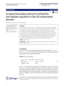
where DRW is the domain of integration in the ξ α plane (image of SRθ in the ξ α plane, defined by W ξ 1 ∈ (0, t − θTE ) and ξ 2 ∈ (ξA2 , ξB2 )), which is obviously a function of x and t, through t − θ. For the sake of clarity, the corresponding shape of SRθ is depicted in Fig. 1 (which is for the hovering– W rotor case discussed in Section 5 and for a prescribed collocation point located at the trailing–edge of the blade, see the black square). The figure shows the lines ξ 1 =constant and ξ 2 =constant, and the line, L(ξA2 , ξB2 ), which separates the contributing portion of the wake surface (solid–line panels) and the non–contributing one (dashed–line panels). In contrast with the assumption made for the body, DRW is not independent of the variables x and t. Thus, moving the derivatives inside the integral sign yields line–integral contributions. Specifically, Z
∇x ·
h DR
W
Z √ i 1 2 ˆ nG∆ϕ a dξ dξ = θ
DR
h √ i ˆ a dξ 1 dξ 2 + ∆IW1 ∇x · nG∆ϕ θ
W
11
(37)
TE
TE
where, noting that (in analogy to Footnote 6) ∇x θTE = er /c(1 − Mr ), with Mr = vTE · er /c, where vTE = ∂yTE /∂τ , " # √ Z Z h i √ 1 a 2 ˆ ˆ G∆ϕ nr G∆ϕ dξ 2 . (38) ∆IW1 = a n · ∇x θTE dξ = − TE 2 2 2 2 θ c 1 − M L(ξ ,ξ ) L(ξ ,ξ ) r θ A B A B Similarly, one obtains Z h B √ i √ i ∂ Z ∂ h Bˆ 1 2 ˆ Mn G∆ϕ a dξ dξ = Mn G∆ϕ a dξ 1 dξ 2 + ∆IW2 , θ θ ∂t DRW DR ∂t W
(39)
TE
where, noting that (in analogy to Footnote 7) 1 − ∂θTE /∂t = 1/(1 − Mr ), Z
∆IW2 =
h
L(ξ 2 ,ξ 2 ) A
√ i ˆ Mn G∆ϕ a
Ã
B
B
θ
∂θ 1 − TE ∂t
!
dξ =
√
"
Z
ˆ Mn G∆ϕ B
2
L(ξ 2 ,ξ 2 ) A
B
a 1 − MrTE
#
dξ 2 .
(40)
θ
The present formulation reduces to that of Ref. 4, for the specific case examined in that paper (i.e., undeformed wake and formulation in the air frame; if this is not the case, the assumption a˙ = 0 does not apply). Next, note that the numerical evaluation of the line–integral contributions (and of the partial– panel contributions) requires considerable attention and involves a low rate of convergence. Thus, it is desirable to consider an alternate formulation that does not yield a line contribution. This may be obtained by using the following description for the wake geometry: y = yW (τ − ξ 1 , ξ 2 , τ ) [ξ 1 ∈ (0, τ ); ξ 2 ∈ (ξA2 , ξB2 )],
(41)
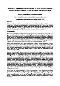
where now the variable ξ 1 originates from the current location of the trailing edge and may be identified with a backward time shift (ξ 1 = τ identifies the material points which, at time τ = 0, were on the trailing edge). For the sake of clarity the resulting shape of SRθ is illustrated in Fig. 2 W (which is for the same problem of Fig. 1 and for the same collocation point); the lines ξ 1 =constant and ξ 2 =constant are also shown. Note that, in this formulation, there is no line–integral contribution, because the integrand vanishes (i.e., ∆ϕ = 0) at the upper limit of integration (i.e., ξ 1 = τ , which corresponds to the initial trailing–edge location).
4
NUMERICAL ALGORITHM
For all the results presented here a zeroth–order discretization is used. Specifically, divide the body and wake surfaces, respectively, into NB and NW quadrilateral elements, assume χˆθ , ϕθ , ϕ˙ θ , ∆ϕθ and ∆ϕ˙ θ to be constant within the respective element, and use the collocation method. This yields N
Ek (t)ϕk (t) =
B X
N
Bkj χˆj (t − θkj ) +
j=1 N
+
W X
n=1
B X
N
Ckj ϕj (t − θkj ) +
j=1
B X
Dkj ϕ˙ j (t − θkj )
j=1
N
Fkn ∆ϕn (t − θkn ) +
W X
Gkn ∆ϕ˙ n (t − θkn )
n=1
12
(42)
with Z
Bkj =
Z θ
Sjθ
Kχˆ (xk , t, zˇ)dS , Ckj =
Z θ
Sjθ
Kϕ (xk , t, zˇ)dS , Dkj =
Sjθ
Kϕ˙ (xk , t, zˇ)dS θ ,
(43)
and similar expressions for Fkn and Gkn . These integrals are evaluated by approximating the surface by a portion of a hyperboloidal paraboloid [which is linear along each coordinate line, see Ref. 16 for details]. The integrals are evaluated analytically whenever possible [see again Ref. 16 for the analytical expressions used for the integration of monopoles and dipoles]; the approximations are of the same order of magnitude as those used for the unknowns. A piecewise linear discretization is used for the time variable, thereby yielding a step–by–step integration scheme. For all the results presented in the next section (single–bladed rotors), we have NB = 2N1 N2 , where N1 denotes the number of elements on the blade along the chord and N2 the number of W W elements along the span, whereas NW = N1 N2 , where N1 denotes the number of wake elements in the azimuthal direction. A subpaneling technique is used for highly distorted element, as it occurs in the Approach C introduced below. Specifically, in this case, each panel is subdivided into NS × NS sub–panels (with obvious increase in computational time). As mentioned above, the pressure is evaluated by Bernoulli’s theorem. Specifically, for all of the aerodynamic results we use the nonlinear compressible Bernoulli theorem, Eq. 6, whereas for aeroacoustics, we use the linearized form p − p∞ = −ρϕ. ˙
(44)
In the following section, we present a series of numerical results. Consider first the formulations used for hovering rotors (i.e., for Figures 3–8). Three formulations are examined. For all three of them, the rotor contribution is evaluated in the body frame of reference. In the first formulation (hereby denoted as Approach A), the wake also is evaluated in the body frame of reference, with respect to which the wake is fixed. In the other two formulations (Approach B and C), the wake contribution is evaluated in a non-rotating frame (see below for details), with coordinates given in Eqs. 35 and 41, respectively. This implies that in Approach B we have a line contribution, which does not appear in Approach C. In the forward flight case we examined two different problems. In the first, we consider a symmetric non–lifting rotor, for which there is no wake; the body contribution is evaluated both in the body and the air frame. Since, these are in good agreement (see Fig. 9), in the lifting forward flight case we limited ourselves to the body frame for the body contribution. On the other hand, for the wake contribution we use the air frame (Approaches B and C).
5 NUMERICAL VALIDATION In this Section, we present results for single–bladed helicopter rotors in hover and forward flight. The objective here is to verify that different formulations give the same results. Indeed, some of the formulations have been validated in the past and are used only for validation of the others. Specifically, for the hovering case, Approach A (with both body and wake contributions evaluated in the body frame) has been validated in the past [see e.g., Ref. 2 and Ref. 17] and is used here as the reference formulation against which to compare the other two. On the other hand, for the 13
forward flight case, Approach B (where the body contribution is evaluated in the body frame, and the wake contribution in the air frame, with coordinates given in Eq. 35) has been validated in the past [see e.g., Ref. 4], and is used here as the reference formulation to validate formulation C. Consider first hovering rotors. The test case chosen for the aerodynamic validation is that already used in Ref. 6, i.e., a one–bladed hovering rotor having a rectangular blade with radius R = 1 m, chord c = 0.1 m, NACA 0012 section, and Mtip = 0.5. The root angle of attack is of 6◦ , whereas the tip angle of attack is of 4◦ . Given the above–stated objective of this validation, all the results presented are obtained for an undeformed wake surface (i.e., neglecting the wake roll–up), with a prescribed pitch. Specifically, in the air frame, the wake points are convected by an induced vertical velocity vW , which for simplicity we assume to be constant; this yields a helicoidal wake, which rotates rigidly, i.e., the wake points move downwards. We chose this test case because it allows one to compare the results obtained with the already validated Approach A, with two novel formulations, including one which requires the use of the emission surface S θ (Approach C, see below). In the second formulation (Approach B), the wake contribution is evaluated in a frame of reference that moves in uniform translation with respect to the air frame, with velocity vW , so that the wake surface is fixed in this frame of reference; the coordinates are those of Eq. 35. This formulation is interesting because it allows one to use analytical expressions for the delays θ and for the integrals over the elements [which are available for surfaces that are fixed in a frame of reference in uniform translation with respect to the undisturbed air, see, e.g., Ref. 16]. In addition, the use of Eq. 35 implies the presence of the line contribution, which in turn requires the use of partial panels [only the contributing portion must be used for the panels intersected by the line L(ξA2 , ξB2 )]. This may be seen from Fig. 1 (introduced in Section 3) which depicts the wake geometry used in this case. In the third formulation (Approach C), the frame of reference is fixed with the undisturbed air. As stated above, in this frame of reference the wake moves in rigid body rotation; the coordinates are those of Eq. 41. This formulation is interesting because it requires the use of the emission (or retarded) surface, which implies highly distorted panels. This may be seen from Fig. 2 (introduced in Section 3), which depicts the wake geometry used in this case. The results obtained with Approach B are presented in Fig. 3, which depicts the convergence analysis of the pressure coefficient distribution (at the blade section located at 0.75 R), as the blade panels are increased. It is apparent that the solution has an excellent rate of convergence and that the solution obtained with N1 = N2 = 14 is very close to the converged one. For these results, W we used two spirals, with 24 elements per spiral (i.e., N1 = 48). These results are virtually indistinguishable from those obtained with Approach A. Hence the formulation of Approach B may be considered validated. Next, consider Approach C. In this case, as stated above, no line contribution appears, but the wake panels are highly distorted. This causes the need for a special algorithm to capture the contributions of such distorted panels. Specifically, in this preliminary analysis, the subpaneling technique described in Section 4 is utilized. The results presented in Fig. 4 are for N1 = 10 and N2 = 6 and different values of NS , and are compared with those of Fig. 3 (again we used two W spirals and N1 = 48). The results are encouraging, as the change in sign in pressure jump for Approach C moves towards the trailing edge. Indeed, the solution approaches that of Approach A, for which there is no pressure jump at the trailing edge (as it may be seen by extrapolating the curves; for a detailed discussion of the trailing edge issues see Ref. 15). However, because of the high values for NS , the sub–panelling technique requires an excessive amount of computer time. 14
Thus, further analysis is warranted. Specifically, a less crude algorithm for the evaluation of the distorted–panel contributions (based on Gaussian quadrature) is being developed. Next, still for the case of hovering rotors, consider a transient response (note that this is still performed with the rigid wake geometry described above – hence these results are exclusively of theoretical interest). In Fig. 5, we compare Approaches A, B, and C, for an unsteady rotor W configuration. Specifically, for N1 = N2 = 14, two spirals, and N1 = 48, Fig. 5 shows the evolution of the circulation ∆ϕTE at the section located at 0.75 R, for a rotor starting from rest, with Mtip = 0.7. As for the steady–state case (see above), the agreement between the Approaches A and B appears to be quite good, whereas Approach C appears to converge slowly to the same results. Note that the highest value used here for NS is 12 (as compared to 70 for Fig. 3). Again, further analysis is warranted. Next, consider some results for the aeroacoustic validation. Still for the hovering case, consider a rotor with a single rectangular blade, a NACA0012 section, radius R = 1.829 m, and chord c = 0.1334 m [akin to that used by Ref. 18, which however has two blades]. The angle of attack at the root is 14.1◦ , the angle of attack at the tip is 4.1◦ , whereas the angular velocity is equal to 135 rad/s, which corresponds to a tip Mach number equal to 0.73. In addition, we have also considered an undistorted helicoidal wake and an observer placed on the rotor disc at a distance of 3 m from the rotor hub. In Fig. 6, we present the acoustic signature obtained with N1 = 8, N2 = 10, and different number of wake spirals, with 180 elements per spiral (the aerodynamic results were obtained with N1 = 8, N2 = 10, five wake spirals, with 48 elements per spiral). From these results, it is apparent that for an accurate acoustic analysis it is necessary to include at least twenty wake spirals. Note that this is in contrast with the aerodynamic predictions (where, for this specific case, three wake spirals proved to be sufficient). Note also that these results have been computed using Approach A, but identical type of convergence has been obtained by using Approaches B and C (see also Fig. 8). Next, consider the convergence analysis of the acoustic signature with respect to the radial discretization (of body and wake). This is presented in Fig. 7, which corresponds to N1 = 8, thirty wake spirals and 180 elements per spiral (five wake spirals, with 48 elements per spiral are used for aerodynamics). In this case, about N2 = 10 span–wise elements appear to give adequately converged results, akin to the aerodynamic analysis. Of course, were we to consider a rolled–up wake (such as that obtained by free–wake analysis) the number of radial elements required for convergence would be much higher, especially for the hovering case (see Ref. 2), and in general for any BVI configuration. Finally, in Fig. 8, we compare the results obtained by using a body frame for the blade, and the above three formulations (Approach A, B and C) for the wake (the results are obtained with discretization used for Fig. 6, for both aerodynamics and aeroacoustics; thirty wake spirals were used for the aeroacoustic calculations). From the figure, it is possible to note that the results obtained by Approaches A and C are in very good agreement, whereas some discrepancies are present in the signal predicted by Approach B. It is worth pointing out that in this case NS = 1 appears adequate, in strong contrast with the aerodynamic analysis (see Fig. 4); this is due to the larger distances between elements and collocation points that exist in the aeroacoustic analysis (as compared to that in aerodynamics, where even singular contributions are present). This implies less time–delay variation over the panels, and hence less distortion. Next, consider the forward–flight case. In this case, we consider different formulations, not only for the wake, but also for the blade. First, we compare air– and body–frame formulations for the body contribution. For simplicity, we considered the simplest possible case, so as to avoid the influence of other unrelated effects. Specifically, we considered a one–bladed rotor, with zero angles of attack, twist and coning, in forward–flight conditions (i.e., with no wake and non–lift), 15
with hovering tip Mach number Mtip = ΩR/c = 0.7 and advance ratio µ = .15. The panels are highly distorted in this case as well, and the subpaneling technique described in Section 4 is again utilized. Consider first a convergence analysis for the air–frame formulation. This is shown in Fig. 9, which depicts the potential distribution, ϕ, at the blade section located at 0.75 R and at the blade azimuthal position Ψ = 90◦ , for N1 = 12, N2 = 6, and different values of NS . It is apparent that, in this case, the solution has a good rate of convergence and the solution obtained with NS = 4 is very close to the converged one. Next, consider a comparison between the air– and the body–frame formulations. This is shown in Fig. 10, which depicts the chordwise potential distribution for two different blade azimuthal positions (Ψ = 90◦ and Ψ = 270◦ ), for the two cases. The agreement between the two formulations appears to be very good. Hence, the air–frame formulation for the body may be considered validated. In view of the fact that the air–frame formulation requires a slightly higher amount of computer time, the remainder of the validation is performed by using the body–frame formulation for the blade, and Approaches B and C for the wake. Specifically, we consider a rotor in ascent forward– flight conditions, with hovering tip Mach number Mtip = 0.7, advance ratio µ = .15 and effective tip–path–plane angle αTPP = 5.75◦ . In particular, for Approach C, consider the convergence analysis in terms of NS . This is shown in Fig. 11, which depicts the circulation ∆ϕTE , at the section located at 0.75 R (these results were obtained with N1 = 12, N2 = 6, and one spiral with W N1 = 12). Again, further analysis is warranted. Moreover, Fig. 12 shows the comparison between Approach B and the NS = 32 case for Approach C. As for the steady–state case, the agreement between the two formulations is quite satisfactory. Finally, consider some results for the aeroacoustic validation. Also in this case, we consider a rotor with a single rectangular blade, a NACA0012 section, radius R = 1. m, and chord c = 0.1 m in ascent forward–flight conditions, with hovering tip Mach number Mtip = 0.7, advance ratio µ = .15 and effective tip–path–plane angle αTPP = 5.75◦ . In addition, we have also considered an undistorted wake and an observer placed on the rotor disc at a distance of 3 m from the rotor hub. Figure 13 shows the acoustic signature obtained with N1 = 8, N2 = 10, and different number of wake spirals, with 180 elements per spiral (the aerodynamic results were obtained with N1 = 8, N2 = 10, five wake spirals, with 48 elements per spiral). In this case, Approach B has a good rate of convergence and the solution presented in Fig. 13 is very close to the converged one. Formulation C appears to converge slowly to the same results. From the figure, it is possible to note that the results obtained by Approaches B and C are in good agreement.
6
CONCLUDING REMARKS
A unified method to analyze aerodynamics and aeroacoustics of bodies in arbitrary motion has been presented and validated, for subsonic tip Mach numbers. The method consists of a boundary integral formulation for the velocity potential for a deformable surface that moves in arbitrary motion with respect to an auxiliary frame of reference, which in turn moves in arbitrary motion. The corresponding boundary integral equation is used for the aerodynamic calculations, whereas the boundary integral representation is used for the aeroacoustic ones [see also Ref. 13, where the relationship between aerodynamics and aeroacoustics is addressed in details, and Ref. 6, where preliminary results limited to aerodynamics are presented]. The present formulation would allow one to overcome drawbacks in the past formulations by the authors [Ref. 2, Ref. 3, and Ref. 4], in which, for rotors in hover, both body and wake are treated in the body frame of reference, whereas
16
for rotors in forward flight the wake is treated in the air frame. Numerical results for the validation includes aerodynamics and aeroacoustics. For helicopter rotors in hover, the blade is evaluated in the body–frame, and the wake in three different frames (see Section 3); for helicopter rotors in forward flight, the blade contribution is considered in both air– and body–frame (for non–lifting rotors), and the wake in two different air–frame formulations (Approaches B and C of Section 3). Hence, the formulation with the blade in the body frame and the wake in the two air–frame formulations has been validated for both rotors in hover and forward flight. These could be used to address, for instance, the transition from hover to forward flight or the conversion phase of a tilt–rotor. As mentioned above these results are still considered as preliminary, as improvements in the algorithm and further validations are highly desirable (and currently underway). In particular, a fair assessment for Approach C will be possible only after the Gaussian quadrature for the evaluation of the distorted–panel contributions has been successfully implemented. Therefore, a CPU comparison appears meaningless at this stage. Finally, we recall that we have introduced the following simplifying assumptions: (1) the flow is assumed linear subsonic, (2) the wake geometry is prescribed, and (3) the blade is rigidly connected with the axis of rotation. These assumptions are legitimate in view of the objective of the paper (i.e., comparison of the different formulations). Nonetheless, the reader might like to know that these are not restrictive assumptions. Indeed, (1) results for transonic flows have been presented in Ref. 17, (2) results for free wake are available in Ref. 19 and Ref. 2 for hover and Ref. 20 for forward flight, and (3) the effects of the blade motion are considered in Ref. 20.
REFERENCES 1. Morino, L., A General Theory of Unsteady Compressible Potential Aerodynamics, NASA CR–2464, 1974. 2. Morino, L., Bharadvaj, B.K., Freedman, M.I., and Tseng, K., Boundary Integral Equation for Wave Equation with Moving Boundary and Applications to Compressible Potential Aerodynamics of Airplanes and Helicopters, Computational Mechanics, 1989, 4, 231–243. 3. Gennaretti, M., Una Formulazione Integrale di Contorno per la Trattazione Unificata di Flussi Aeronautici Viscosi e Potenziali, PhD Thesis in Theoretical and Applied Mechanics, University of Roma “La Sapienza”, 1993. 4. Gennaretti, M., Luceri, L., and Morino, L., A Unified Boundary Integral Methodology for Aerodynamics and Aeroacoustics of Rotors, Journal of Sound and Vibration, 1997, 200, 467–489. 5. Morino, L., Bernardini, G., Gennaretti, M., Integrated Aerodynamic/Aeroacoustic Analysis of a Tiltrotor During Conversion, AIAA Paper 2000–2028, 6th AIAA/CEAS Aeroacoustic Conference, Lahaina, Hawaii, 2000. 6. Morino, L., Bernardini, G., Gennaretti, M., A Boundary Element Method for the Aerodynamic Analysis of Aircraft in Arbitrary Motions, accepted for publication in Computational Mechanics (also presented at IABEM 2002, International Association for Boundary Element Methods, UT Austin, TX, USA, May 28–30, 2002), 2003. 17
7. Ffowcs Williams, J.E., and Hawkings, D.L., Sound Generation by Turbulence and Surfaces in Arbitrary Motion. Philosophical Transactions of the Royal Society, 1969, A264(1151), 321–542. 8. Farassat, F., Theory of Noise Generation from Moving Bodies with an Application to Helicopter Rotors, NASA TR–R–45, 1975. 9. Farassat, F., and Myers, M.K., Extension of Kirchhoff’s Formula to Radiation from Moving Surfaces, Journal of Sound and Vibration, 1988, 123, 451–460. 10. Brentner, K.S., Numerical Algorithms for Acoustic Integrals with Examples for Rotor Noise Prediction, AIAA Journal, 1997, 35(4), 625–630. 11. George, A.R., and Lyrintzis, A.S., Mid–Field and Far–Field Calculations of Transonic Blade– Vortex Interactions, AIAA Paper 86–1854, AIAA 10th Aeroacoustics Conference, Seattle, WA, 1986. 12. Lyrintzis, A.S., Review: The Use of Kirchhoff’s Method in Computational Aeroacoustics, ASME Journal of Fluids Engineering, 1994, 116(4), 665–676. 13. Morino, L., Is There a Difference Between Aeroacoustics and Aerodynamics? An Aeroelastician’s Point of View, keynote lecture at the 8th AIAA/CEAS Aeroacoustics Conference in Breckenridge, CO, USA, June 2002. Accepted for publication in the AIAA Journal, 2003. 14. Morino, L., and Gennaretti, M., Boundary Integral Equation Methods for Aerodynamics. In: Atluri SN (ed), Computational Nonlinear Mechanics in Aerospace Engineering (Progress in Aeronautics and Astronautics), American Institute of Aeronautics and Astronautics, 146, 1992, 279–320. 15. Morino, L., and Bernardini, G., Singularities in BIE’s for the Laplace Equation; Joukowski Trailing–Edge Conjecture Revisited, Journal of Engineering Analysis with Boundary Elements, 2001, 25, 805–818. 16. Morino, L., Chen, L.T., and Suciu, E.O., Steady and Oscillatory Subsonic and Supersonic Aerodynamics Around Complex Configurations, AIAA Journal, 1975, 13(3), 368–374. 17. Morino, L., Gennaretti, M., Iemma, U., and Salvatore, F., Aerodynamics and Aeroacoustics of Wings and Rotors via BEM – Unsteady, Transonic and Viscous Effects, Computational Mechanics, 1998, 21(4/5), 265–275. 18. Brentner, K.S., Prediction of Helicopter Rotor Discrete Frequency Noise, A Computer Program Incorporating Realistic Blade Motions and Advanced Acoustic Formulation, NASA TM–87721, 1986. 19. Morino, L., Kaprielian, Z., Jr., and Sipcic, S.R., Free Wake Analysis of Helicopter Rotors. Vertica, 1985, 9 (2), 127–140. 20. Gennaretti, M., Corsetti, E., and Morino, L., Coupled Free–Wake–Aerodynamics/Blade– Dynamics Analyses of Rotors in Forward Flight, AIAA Paper 98–2241, 4th AIAA/CEAS Aeroacoustic Conference, Toulouse, France, 1998.
18
L (ξ
1 ξ =0
2 A
,ξ B) 2
ξ
1
ξ
2
Figure 1: Wake emission surface SWθ for a hovering rotor (Approach B)
19
ξ=0 1
ξ
2
ξ
1
Figure 2: Wake emission surface SWθ for a hovering rotor (Approach C)
20
0.2
pressure coefficient
0
-0.2
-0.4
N 1xN 2 = 10x6 N 1xN 2 = 12x10 N 1xN 2 = 14x14 N 1xN 2 = 16x18
-0.6
-0.8
-1 0.0
0.25
0.5
0.75
dimensionless chordwise abscissa
Figure 3: Chordwise pressure coefficient distribution at r = .75R, for Mtip = 0.5 (Approach B)
21
1.0
0.4
0.2
pressure coefficient
0
-0.2
-0.4
body frame N S= 10 N S= 30 N S= 70
-0.6
-0.8
-1 0.0
0.25
0.5
0.75
dimensionless chordwise abscissa
Figure 4: Chordwise pressure coefficient distribution at r = .75R, for Mtip = 0.5 (Approach C)
22
1.0
1.8 Approach A Approach B Approach C (N S = 2) Approach C (N S = 4) Approach C (N S = 8) Approach C (N S = 12)
1.6
circulation
1.4
1.2
1
0.8
0.6 0
10
20
30
40 time steps
50
60
70
80
Figure 5: Time history of circulation, ∆ϕTE , at r = .75R for Mtip = 0.7 (Approaches A, B, and C)
23
20 15
acoustic signature (Pa)
10 5 0 -5 5 spirals 10 spirals 20 spirals 40 spirals
-10 -15 -20 -25 0
40
80
120
160 200 240 azimuthal position (deg)
280
320
360
Figure 6: Convergence analysis with respect to the wake length for the acoustic signal at observer location r/R = 3 and Mtip = 0.73 (Approach A)
24
10
acoustic signature (Pa)
5
0
-5 N2 = 6 N2 = 8 N 2 = 10 N 2 = 12
-10
-15
-20
-25 0
40
80
120
160 200 240 azimuthal position (deg)
280
320
360
Figure 7: Convergence analysis with respect to spanwise wake elements for the acoustic signal at observer location r/R = 3 and Mtip = 0.73 (Approach A)
25
10
5
acoustic signature (Pa)
0
-5
-10
Approach A Approach B Approach C
-15
-20
-25
-30 0
40
80
120
160 200 240 azimuthal position (deg)
280
320
360
Figure 8: Acoustic signal at observer location r/R = 3 and Mtip = 0.73 (Approaches A, B and C)
26
0.6 NS = 2 NS = 4
0.4
potential
0.2
0
-0.2
-0.4
-0.6
-0.8 0.0
0.25
0.5 dimensionless chordwise abscissa
0.75
1.0
Figure 9: Convergence analysis of potential, ϕ, at r/R = 0.75, Mtip = 0.7 and Ψ = 90◦ (Approach C)
27
0.6
Ψ = 90 0
0.4
0.2
potential
Ψ = 270 0 0
-0.2 body frame air frame
-0.4
-0.6
-0.8 0.0
0.1
0.2
0.3
0.4 0.5 0.6 0.7 dimensionless chordwise abscissa
0.8
0.9
1.0
Figure 10: Potential, ϕ, on blade at r/R = 0.75, Mtip = 0.7 (Approaches A and C)
28
1.8 NS = 2 NS = 4 NS = 8 NS = 16 NS = 32
1.6
circulation
1.4
1.2
1
0.8
0.6 0
5
10
15
20
25
30
35
time steps Figure 11: Convergence analysis of circulation, ∆ϕTE , at r/R = 0.75 and Mtip = 0.7 (Approach C)
29
1.6 Approach B Approach C 1.5
circulation
1.4
1.3
1.2
1.1
1
0.9 0
5
10
15
20
25
30
35
time steps
Figure 12: Time history of the circulation, ∆ϕTE , at r/R = 0.75 and Mtip = 0.7 (Approaches B and C)
30
2 1 0
acoustic signature (Pa)
-1 -2 -3 -4
Approach B Approach C (NS = 5) Approach C (NS = 20) Approach C (NS = 50)
-5 -6 -7 -8 0
40
80
120
160
200
240
280
320
360
azimuthal position (deg)
Figure 13: Convergence analysis with respect to the wake length for the acoustic signal at observer location r/R = 3 and Mtip = 0.7
31