A branch-and-bound algorithm for single machine ...

*Manuscript Click here to view linked References

A branch-and-bound algorithm for single machine scheduling with quadratic earliness and tardiness penalties K. Kianfar a,1 , G. Moslehi a a

Department of Industrial and Systems Engineering, Isfahan University of Technology, 84156-83111, Isfahan, Iran

Abstract This paper considers the problem of scheduling a single machine, in which the objective function is to minimize the weighted quadratic earliness and tardiness penalties and no machine idle time is allowed. We develop a branch and bound algorithm involving the implementation of lower and upper bounding procedures as well as some dominance rules. The lower bound is designed based on a lagrangian relaxation method and the upper bound includes two phases, one for constructing initial schedules and the other for improving them. Computational experiments on a set of randomly generated instances show that one of the proposed heuristics, used as an upper bound, has an average gap less than 1.3% for instances optimally solved. The results indicate that both the lower and upper bounds are very tight and the branch-and-bound algorithm is the first algorithm that is able to optimally solve problems with up to 30 jobs in a reasonable amount of time.

Keywords: Scheduling, Single machine, Quadratic earliness and tardiness, Branch-and-bound

1. Introduction and problem definition Scheduling models involving both earliness and tardiness penalties are consistent with the just-in-time production philosophy in the sense that they force jobs to be completed as close to their due dates as possible. This paper examines a model including both earliness and tardiness penalties in a quadratic form. Therefore, jobs that are quite early or tardy are heavily penalized. The advantage of a quadratic penalty function (compared to a linear one) is twofold. First, it avoids schedules where only a few jobs contribute to the majority of the penalty. Second, quadratic penalties better reflect reality, because in many practical situations, the penalties increase in a non-linear (quadratic) way. We consider our problem in a single machine environment that plays a key role in scheduling theory. Single machine problems appear to arise frequently in practice. Also, the performance of some production systems is only dictated by a single machine that is a bottleneck. Consequently, solution procedures for complex systems often require solving single machine sub-problems. Here, it is assumed that no idle time is allowed since machines and jobs must be continuously processed from time zero. This assumption simplifies the problem compared to the general form that allows inserted idle times. This assumption holds in many production systems where the machine cost of being kept idle is larger than the early cost incurred by completing a job before its due date, or the machine is heavily loaded, so that it must be kept running and no idle time is permitted. 1

Corresponding author: Tel.: +98 0311 3915522; fax: +98 0311 3915526

E-mail address: [email protected] (K. Kianfar).

(1)

Formally, the considered problem can be stated as follows: a set of n independent jobs j  1, 2,..., n , has to be scheduled on a single machine that can handle at most one job at a time. We assume that the machine is continuously available from time zero onwards, and preemptions are not allowed. Job j requires a processing time p j and has a corresponding due

date d j . The earliness and tardiness of job j are defined as E j  max 0, d j  C j  and

T j  max 0,C j  d j  respectively, where C j is the completion time of job j. The objective is to

find a schedule that minimizes the sum of weighted quadratic earliness and tardiness penalties, considering that no idle time for machines is allowed. According to the above assumptions, this problem can be represented as 1   h j E j2 w jT j2  . If each job has equal earliness and tardiness penalties, then the problem is simplified to the problem of minimizing a weighted quadratic lateness on a single machine.

2. Literature review The scheduling problem with no idle time and weighted linear earliness and tardiness penalties has been considered by several authors and both heuristic and exact methods have been developed. Among the heuristics, some dispatching rules and beam search algorithms are presented by Ow and Morton [1] and Valente and Alves [2, 3]. Among the exact solution methods, branch-and-bound algorithms are presented by Li [4] and Liaw [5] using a lagrangian relaxation method to get lower bounds. Baker and Scudder [6], provide a comprehensive survey of scheduling problems with earliness and tardiness penalties. Problems with a quadratic objective function have also been investigated in previous studies. Minimization of quadratic lateness, where the lateness of a job is defined as the difference between its completion time and due date is analyzed by Gupta and Sen [7] and Chung et al. [8]. They present a branch-and-bound and a heuristic method for the problem with no idle time. Su and Chang [9] and Schaller [10] consider idle time insertion, and propose timetabling procedures and heuristic algorithms, respectively. Sen et al. [11] develop a branch-and-bound algorithm for the weighted version of quadratic lateness penalties, where idle time is allowed only prior to the start of the first job. Soroush [12] studies the problem of finding an optimal sequence that minimizes a weighted quadratic function of job lateness on a single machine where idle time is allowed to be inserted only before the processing of the first job begins. Single machine scheduling problems with linear earliness and quadratic tardiness penalties have been previously studied by many researchers. Valente [13] develops a branch-andbound algorithm, as well as a lower bounding procedure based on relaxing the jobs completion times. Among the heuristics, both dispatching rules and beam search heuristics have been proposed by Valente [14, 15]. The above problem is considered by Valente and Goncaclves [16] who present a genetic algorithm approach based on a random key alphabet. Schaller [17] studies the corresponding problem with inserted idle time and develops a branch-and-bound and some heuristic algorithms, as well as a timetabling procedure which optimally inserts idle time in a given sequence. The problem considered in this paper has been previously studied and both exact and heuristic approaches have been developed; however, our computational results indicate that both the heuristic and branch-and-bound methods outperform the previous studies. Valente and Alves [18] consider the single machine problem with quadratic earliness and tardiness costs, and no machine idle time. They present four groups of dispatching heuristics, as well as simple improvement procedures and analyze their performance on a wide range of instances. Some greedy randomized dispatching heuristics are developed by Valente and Moreira [19] which differ on the strategies involved in the construction of the greedy randomized (2)

schedules, and also on whether they employ only a final improvement step or perform a local search after each greedy randomized construction. Valente [20] presents a branch-and-bound algorithm which is capable of finding optimal solutions for problems with up to 20 jobs. He proposes two different lower bounds, as well as a procedure that combines these two lower bounds. The first lower bound is designed based on a relaxation of earliness and tardiness penalties and completion times. The second lower bound first converts the original early/tardy objective to a weighted quadratic lateness objective after which the lower bounding procedure proposed by Sen et al. [11] is used for the modified problems. The initial upper bound is calculated using the ETP_v2 (early/tardy priority-version2) dispatching rule, followed by the application of a 3-swap improvement procedure both presented by Valente and Alves [18]. The single machine scheduling problem with quadratic earliness and tardiness penalties is studied via developing some beam search heuristics by Valente [21]. These heuristics consist of classic beam search procedures, as well as filtered and recovering algorithms. They consider three dispatching heuristics as evaluation functions, in order to examine the effect of different rules on the performance of the beam search algorithms. The single machine scheduling problem with uncertain processing times is considered by Xia et al. [22] where the objective is to minimize a combination of quadratic earliness, tardiness and due date assignments. Table 1 reviews some studies on the problems with linear and quadratic objectives. In this table, DR, Heu, BS, B&B, DP and GA respectively denote dispatching rule, heuristics, beam search, branch-and-bound, dynamic programming and genetic algorithm. Also, r j , d and Var denote release time, common due date and variance, respectively. Table 1: List of studies on the problems with linear and quadratic objectives Reference

idle time

[1]

No

[2]

No

[3]

No

[4]

No

[5]

No

[7]

No

[8] [9] [10] [11] [12] [27] [28]

No Yes Yes before first job before first job No No

[29]

No

[30]

No

Objective function Approach

h E h E h E h E h E L L L L w L w L C w C w C w C

Reference

idle time

Objective function

Approach

w C j  rj  2 w C j  d 

j

j

 w jT j 

DR

[23]

No

j

j

 w jT j 

Heu

[24]

Yes

j

j

 w jT j 

BS

[25]

No

Var C j 

DP

j

j

 w jT j 

B&B

[26]

No

Heu

j

j

 w jT j 

T

B&B

[13]

No

B&B , Heu

[14]

No

2

j

2

j

2

j

2

j

j

2

j

j

[16]

B&B , heu

j

2

j

[15]

B&B , Heu

j

2

2 j 2

j

j

j

j

2

No No

B&B , heu

[17]

Yes

B&B

[18]

No

B&B

[19]

No

Heu

[20]

No

[21]

Heu

[22]

B&B B&B

No No

This study No

(3)

2

B&B

j

Heu

j

2 j

h E h E h E h E h E h E h E h E h E h E h E

j

 w jT j

2

j

j

 w jT j

2

j

j

 w jT j

2

j

 w jT j

2

j

j

 w jT j

2

j

 w jT j

2

j

j

 w jT j

2

j

j

 w jT j

2

j

 w jT j

2

j

j

j

2

2

2

2 j 2

j

j

j

j

2

        

B&B DR BS GA B&B , heu heu heu B&B BS

 w jT j  yD j 2

 w jT j

2

2





heu B&B , heu

The remainder of this paper is organized as follows. The next section describes a heuristic algorithm including two phases of construction and improvement. In section 4, we present the branch-and-bound and related bounding procedures and dominance rules. The computational results are reported in section 5. Finally, we provide some concluding remarks in section 6.

3. Heuristic algorithm In this section, a heuristic method will be developed to provide near optimal solutions for the problem 1 | | h j E j2 w jT j2 . This method includes two main phases. In the first phase, an initial sequence is built applying a constructive procedure and in the second phase, the initial solutions are improved by an improving algorithm. 3.1. Constructive phase Algorithm1 is the constructive procedure which is based on the NEH (Nawaz, Enscore and Ham) algorithm [31].

Algorithm 1 Step 1: Renumber the jobs according to the non-decreasing order of their due dates. Step 2: Schedule the first job to the beginning of the sequence and calculate the related earliness or tardiness penalty. Set i  2 . Step 3: Check the ith job to be inserted in i possible positions in the sequence and calculate the related penalty for each job position. Schedule the ith job into the position with the minimum total penalty of all the i jobs. Step 4: If i  N then the final sequence is obtained, and stop, else set i  i  1 and go back to step 3.

3.2. Improvement phase First, a lemma and a theorem are introduced as the foundations of improving algorithm 2. Lemma 1: Suppose a set of adjacent jobs have a fixed order and starting time t and E i t  and T i t  denote the earliness and tardiness of job i in this set. If the sub-sets of early and tardy jobs in this set are denoted by G E (t ) and GT (t ) respectively, then the function F (t )  i G (t )  hi E i (t )    j G (t ) w jT j (t )  will be continuous and decreasing and there is a E

T

real value t  t such that F (t * )  0 . *

Proof: See Appendix A. □ Theorem 1: Suppose a set of adjacent jobs have a fixed order and starting time t. Let Z t  be the sum of quadratic earliness and tardiness penalties for this set. The function Z t  is continuous and convex. Proof: See Appendix A. □ Algorithm 2 takes an initial sequence and tries to improve it by shifting groups of adjacent jobs with a fixed order. In steps 3 and 8 of this algorithm, we have used the results concluded (4)

from Theorem 1. Theorem 1 shows that Z t  is a convex function, so if we shift a group of fixed ordered adjacent jobs as much as one unit time to the beginning (end) of a sequence and the penalty function increases, then shifting more than one unit will not improve the penalty. According to this, Algorithm 2 iteratively checks some swaps between jobs that may improve the initial solution.

Algorithm 2 Step 1: Start from the end of the initial sequence and call the first tardy job i. Step 2: If swapping job i and the job immediately before i improves the penalty function, then swap them and go back to step 2, else go to step 3. Step 3: Let job j be the nearest tardy job before job i and group jobs i and j and all the jobs between them as group G. Check all the jobs in group G to be shifted one unit time to the beginning of the sequence and recalculate the penalty. If the penalty decreases, then go to step 4, else go to step 5. Step 4: Let job k be the nearest early job before group G. Check swapping job k with all tardy jobs in group G and select the swap with the most decrease in penalty function. Step 5: If there is any tardy job before job i, consider the nearest one to job i as a new job i and return to step 2, else the first phase of the algorithm is completed and go to step 6. Step 6: Start from the beginning of the initial sequence and call the first early job i. Step 7: If swapping job i and the job immediately after i improves the penalty function, then swap them and back to step 7, else go to step 8. Step 8: Let job j be the nearest early job after job i and group jobs i and j and all the jobs between them as group G. Check all the jobs in group G to be shifted one unit time to the end of the sequence and recalculate the penalty. If the penalty decreases, then go to step 9, else go to step 10. Step 9: Let job k be the nearest tardy job after group G. Check swapping job k with all early jobs in group G and select the swap with the most decrease in penalty function. Step 10: If there is any early job after job i, consider the nearest one to job i as a new job i and return to step 7, else stop.

4. Branch-and-bound algorithm To propose an efficient branch-and-bound algorithm, we take some policies into consideration in order to reduce the search space. We investigate these policies in the next three sub-sections, and then we will introduce the main branch-and-bound algorithm with depth-first strategy. 4.1. Lower bounding procedure In this section, we develop a multiplier adjustment method to derive an efficient lower bound for the problem 1| | h j E j2  w jT j2 . First, we formulate the problem, decompose it into two sub-problems with a simpler structure, and then use the multiplier adjustment method for (5)

each sub-problem. The sum of the two lower bounds obtained from both sub-problems is a new lower bound for the main problem. Let E j , ,T j , and C j , be the earliness, tardiness and completion time of job j under sequence  , respectively. The main problem (V) is logically formulated as follows where  indicates the set of all possible sequences. N



V *  Min  h j E j2,  w jT j2,  

j 1

s .t . E j ,  0



E j ,  d j  C j ,

T j ,  0

j  1, 2,..., N

T j ,  C j ,  d j

(1)

j  1, 2,..., N

With only early costs or tardy costs considered in the objective function, problem V can be decomposed into two sub-problems V1 and V2 as follows. N



V 1*  Min  w jT j2,  

i 1

s .t . T j ,  0

(2) T j ,  C j ,  d j N



V 2*  Min  h j E j2,  



j 1

s .t . E j ,  0

j  1, 2,..., N

 (3)

E j ,  d j  C j ,

j  1, 2,..., N

The above two sub-problems have a simpler structure than the main problem, and appear easy to solve. As any feasible solution to problem V is also feasible to sub-problems V1 and V2 , we have V 1* V 2* V * . Suppose LowerT is a lower bound for V 1 and LowerE is a lower bound for V 2 , then LowerE  LowerT V 1* V 2* V * and the decomposition will give a lower bound for the main problem. The lower bounds related to sub-problems V1 and V2 will be described in sections 4.1.1 and 4.1.2.

4.1.1. Derivation of the lower bound for sub-problem V1 Relaxing the second constraint in V1 yields the lagrangian sub-problem R1.





R1   j   Min   w jT j2,   jT j ,   j C j ,  d j   N

 

j 1

s .t . T j ,  0

(4)

j  1, 2,..., N

As pointed out by Li [4], for any choice of nonnegative  , R1   j  provides a lower bound for V1. The objective function in R1 can be rewritten as follows.

(6)

R1   j   Min  w jT j2,   jT j ,      j C j ,      j d j   

N

N

N

j 1

j 1

j 1

T j ,  0

j  1, 2,..., N

Minimum value of the first term in equation (5),

 w N

j 1

j

T j , 

2w

(5)

 j2

yielding the minimum value

4w

j

j



T j2,   jT j , , is obtained by setting

. The second term denotes the weighted sum of

j

completion times which is minimized by WSPT (Weighted Shortest Processing Time) order of jobs. WSPT order is obtained by making all the adjacent jobs j and j+1 satisfying  j   j 1 . pj

p j 1

The third term is constant under any selection of  j values. Replacing the first term in R1   j  with its optimal value  j2 4w j , will give a quadratic

and convex function called R1   j  . The minimum value of R1   j  in the optimality condition can be obtained by calculating the first order derivation of this function as follows.  R1  j   j  (C j ,  d j )  0   j  2w j (C j ,  d j ) (6)  j 2w

 

j

The multiplier adjustment method is a common technique to compute values of the lagrangian multipliers  j . This method firstly requires a heuristic to sequence the jobs, and then chooses the multipliers so that the resulting lower bound is as large as possible. Here, the WSPT rule is selected as an initial sequence and from now on, we assume that the jobs are renumbered so that the sequence generated by the WSPT rule is (1,2,...,n). WSPT is very simple and efficient in producing a sequence and, in our computational studies, often results in tighter lower bounds. Hence, index  is dropped and the lagrangian dual sub-problem D1 is given in equation (7). N

D1  Min   j  2w j 1

j

C

j

d j 

s .t .

j pj



 j 1 p j 1

0  j

j  1, 2,..., N  1

(7)

j  1, 2,..., N

The term 2w j C j  d j  is constant for each job j and can be replaced by  j for ease of exposition. After the lagrangian dual sub-problem D1 is solved, using the optimal values of multipliers   *j  we can obtain the lower bound as follows.

   *  2  j LowerT     *j C j  d j    j 1  4w j   N

(8)

In the following, we will present an algorithm that optimally solves the sub-problem D1 in a polynomial time. Before that, we present some theorems which construct the foundation of this algorithm. (7)

Definition 1: Define  as a set of k adjacent jobs {1,2,...,k} in a sequence such that 1  2    ...  k . Assume that the jobs are renumbered according to their position in a p1

p2

pk

sequence. Theorem 2: In any optimal solution for the lagrangian dual sub-problem D1 , the set  of jobs J 1 to J k can be decomposed into three sub-sets  1 ,  2 and  3 (see Figure 1) in such a way that the following relations hold. j   1 :  j   j j    2 :  j    j  j    3 :  j    j 

Proof: See Appendix A. □

J1

Ju

1

Jv

2

Jk

3

Figure 1: Set  and its sub-sets  ratios are the same for all jobs in set  . This value is denoted by   p from now on. This means 1  2    ...  k    (9) p1 p 2 pk

Theorem 3: The

Proof: See Appendix A. □ Theorem 4: In any optimal solution for D1 , sub-set  2 cannot be empty; meaning that at least one job j exists in set  satisfying  j   j . Proof: See Appendix A. □ Theorem 5: In any optimal solution for D1 , the following condition holds for the jobs in any set  .  p j   p j    p j  j  2

j 1

 p   p

j 1

j

j 

2

j  3

j

  p j 

(10)

j  3

Proof: See Appendix A. □ Now, according to the above theorems, we propose an algorithm that solves the problem D1 requiring a polynomial computational effort. In this algorithm, jobs sequenced based on WSPT order are grouped into some groups S k , and a value  k is assigned to each group.

(8)

Algorithm 3 Step 1: Set  0  0 and k  0 Step 2: For each job i from the end of the sequence to the beginning, if

i  S k else k  k  1 , i  S k and  k  i .

i pi

  k then set

pi

Step 3: Let K be the number of groups generated in the previous step. Set k  K . Step 4: If



j S k ,

j

pj

pj 



j S k ,

 k

j

p j

p j  go to step 5, else set k  k 1 and if k  1 return to  k

step 4, else go to step 6.    j  Step 5: Set  k   | j  arg min  p i  k  i   . If  k   k 1 then S k 1  S k 1 S k , k  k 1.  i S k , i  k pj  pi   Go back to step 4.

Step 6: The optimal values for the lagrangian multipliers are obtained using *j  p j . k , j  S k .

Theorem 6: Algorithm 3 optimally solves the lagrangian dual sub-problem D1 . Proof: See Appendix A. □ Replacing the lagrangian multipliers from Algorithm 3 in equation (8) will give a lower bound for sub-problem V 1 .

4.1.2. Derivation of the lower bound for sub-problem V2 Similar to the previous section, we use the lagrangian multiplier adjustment method to calculate a lower bound for sub-problem V2. The lagrangian sub-problem R2 for this case is





R 2   j   Min   h j E j2,   j E j ,   j d j  C j ,   N

 

j 1

s .t . E j ,  0

(11) j  1, 2,..., n

Consider the WLPT (Weighted Longest Processing Time) order as an initial sequence in which

j



 j 1

p j p j 1 is as follows.

for any two adjacent jobs j and j+1. Hence, the lagrangian dual sub-problem

(9)

D 2  Min   j  2h j d j  C j  N

j 1

s .t

j pj



 j 1

j  1, 2,..., N  1

p j 1

0  j

(12)

j  1, 2,..., N

Note that the term 2 h j d j  C j  is constant for any job j and can be replaced by  j . Using the WLPT initial order, Algorithm 4 can be used for calculating the optimal values of lagrangian multipliers for sub-problem D2.

Algorithm 4 Step 1: Set  0  0 and k  0 Step 2: For each job i from the beginning of sequence to the end, if i   k then set i  S k pi

else k  k  1 , i  S k and  k  i . pi

Step 3: Let K be the number of groups generated in the previous step. Set k  0 . Step 4: If



j S k ,

j

pj

pj   k



j S k ,

j

p j

p j  go to step 5 else set k  k  1 and if k  K return to  k

step 4 else go to step 6.   Step 5: Set  k   j | j  arg min i  p i  k  i S k , i  k pj pi  Go back to step 4.

  . If  k   k 1 then S k 1  S k 1 S k , k  k 1.  

Step 6: The optimal values for lagrangian multipliers are obtained using *j  p j . k , j  S k . Finally, the lower bound for sub-problem V2 is calculated using equation (13). 2  N   *  j  *  LowerE     j d j  C j     4 h j 1 j  

(13)

4.2. Dominance rules Definition 2: Define  E  T  as a set of adjacent early (tardy) jobs in a sequence such that all the jobs in this set remain early (tardy) under any arbitrary order. Suppose the set  E

 T  includes jobs from positions

m1 to m 2 of a sequence and t is the start time of this set,

then we can formally define set  E  T  as follows.

(10)

 

 E : J j | t   

  p j   d j , j  m1 ,..., m 2  j  m1 ,..., m 2  



(14)

T : J j | t  p j  d j , j  m1 ,..., m 2 

(15)

Theorem 7: Let jobs i and j be two jobs in the set  E  T  respectively, and also suppose that the start time of job i and the time distance between the two jobs are denoted by i and





 , respectively. If i   E i , j  i  T i , j  then the sum of penalties of these two jobs will be





reduced by swapping them, where the parameter  E i , j  T i , j  is calculated as follows.

 E 

T

i ,j 

i ,j 

1 1     hi  p j     d i  p i   p j      h j  p i     d j  p j   p i     2 2      hi  p j     h j  p i   

(16)

1 1     w i  p j     d i  p i   p j     w j  p i     d j  p j   p i     2 2      w i  p j    w j  p i   

(17) □

Proof: The proof is performed using simple interchange arguments.

Result 1: Let jobs i and j be two adjacent jobs in the set  E  T  and suppose that the



start time of the first job (job i) is denoted by i . If i  E i , j  i  T i , j 



then the sum

penalties of jobs i and j will be reduced by swapping them, where the parameter  E i , j 

    is calculated as follows. T i ,j

E

T 

i ,j 

i ,j 

1  1    hi p j  d i  p i  p j   h j p i  d j  p j  p i  2  2     hi p j  h j p i

(18)

1  1    w i p j  d i  p i  p j  w j p i  d j  p j  p i  2  2     w i p j w j p i

(19)

For the sake of brevity, we define hi p j  d i  pi  1 p j   h j pi  d j  p j  1 pi  and hi p j  h j pi 

respectively as 

E1 (i , j )

and w i p j w j pi as 

and 

T1 (i , j )

E2 (i , j )

and 

2





2



. Similarly, we define w i p j  d i  pi  1 p j  w j pi  d j  p j  1 pi  2 2

T2 (i , j )









.

4.3. Main procedure of branch-and-bound In this paper, in addition to the constructive and improving algorithms 1 and 2, we adopt a constructive dispatching rule called ETP_v2 and an improving procedure called 3SW from the study by Valente et al. [18]. These two methods are the most effective ones among the several alternatives investigated in [18]. For the sake of brevity, we signify the constructive (11)

Algorithm 1 and ETP_v2 by Heu1 and Heu4, respectively. Combining the constructive Algorithm 1 (Heu1) with the improving Algorithm 2 and 3SW, two heuristic methods for the problem 1|| h j E j2 w jT j2 called Heu2 and Heu3 will be yielded, respectively. Also, by combining ETP_v2 with Algorithm 2 and 3SW methods, another two heuristics called Heu5 and Heu6 will be obtained, respectively. Let LB1 denote the lower bound described in section 3. Another lower bound for the problem is adopted from the study by Valente [20] called LB_ET. They compared this lower bound with another lower bound and concluded that LB_ET outperforms the other one for the most of the instances. We will signify the LB_ET method as LB2 during the rest of this paper. Two dominance rules are inferred from Result 1 in section 4.2; one for early jobs and the other one for tardy jobs. These two dominance rules are respectively denoted by DOM1 and DOM2 from now on. We design the third dominance rule for the branch-and-bound algorithm (DOM3) based on checking the insertion of the first unscheduled job before a certain number of last scheduled jobs (denoted by  ) and selecting the sequence with the smallest penalty. Table 2 summarizes the heuristic algorithms, lower bounds and dominance rules included in the branch-and-bound algorithm and computational experiments. Table 2: A summary of heuristics, lower bounds and dominance rules Name

Description

Name

Description

Heu1 Heu2 Heu3 Heu4 Heu5 Heu6

Algorithm 1 Algorithm 1 + Algorithm 2 Algorithm 1 + 3SW in [18] ETP_v2 in [18] ETP_v2 in [18] + Algorithm 2 ETP_v2 in [18] + 3SW in [18]

LB1 LB2 DOM1 DOM2 DOM3

Lower bound in section 3 LB_ET in [18] Dominance rule in section 4.2 for early jobs Dominance rule in section 4.2 for early jobs Dominance rule in section 4.3

The branch-and-bound algorithm is designed based on depth-first strategy, where the three dominance rules (DOM1, DOM2 and DOM3) and the two lower bounds (LB1 and LB2) are checked to reduce the search space. The initial upper bound for this algorithm is the best solution obtained from heuristics H2, H3 and H5. The steps of the branch-and-bound algorithm are described as follows. Step 1: Input the initial value for  . Step 2: Determine the upper bound (UB) according to the best sequence created by the heuristic algorithms H2, H3 and H5. Step 3: The set of all jobs is divided into two sets of arranged jobs  and non-arranged jobs   at the beginning and at the end of the sequence, respectively. Let  be the number of jobs in  . Each possible selection of arranged set  and non-arranged set   creates a node in the search tree. Step 4: If the tree is completely searched then go to step 14, else let i be the last job in set  and branches be created in a node with job i as the last scheduled job. Let job j be a member of the set   and denote a new node as    j    ,    j    . The branch ij in the tree is a partial sequence in which job j is located exactly after job i.

(12)

Step 5: If job j is early (tardy), create set  E  T  of job j and some of its previous jobs according to Definition 2. Suppose  E T  is the number of jobs in set  E  T  . Set  j ,k  0 .

Step 6(DOM2 checking): If job j is tardy, for jobs k from position  to  T  2 : swap jobs j and k and calculate the changes in the total penalty as  j ,k   k .T( k1, j )  T( k2, j ) according to Result 1. If  j ,k  0 go to step 13. , Step 7(DOM1 checking): If job j is early, for jobs k from position  to  T  2 : swap jobs j and k and calculate the changes in the total penalty as  j ,k   k .T( k1, j )  T( k2, j ) according to Result 1. If  j ,k  0 go to step 13. , Step 8(DOM3 checking): For jobs k from position   max E ,T   2 to    , swap jobs j and k and if the related penalty decreases, go to step 13. Step 9: Calculate the total penalty of set  as Z      hi E i2 w iT i 2  . i 

Step 10(LB1 checking): Calculate the first lower bound for set   , LB1   , and if Z    LB1    UB go to step 13.

Step 11(LB2 checking): Calculate LB 2   , and if Z    LB 2    UB , go to step 13. Step 12: If     , then calculate the objective function value for the complete sequence of  . If this value is smaller than UB, then assign this value to UB. Go to step 4. Step 13: Eliminate the branch ij and    j    ,    j    and then go to step 4. Step 14: Return the best UB value obtained from the algorithm and stop.

5. Computational results To show the efficiency of the bounding procedures and the branch-and-bound algorithm, it is necessary to design some groups of test problems with different levels of parameters. 5.1. Experimental design The branch-and-bound algorithm is tested on problems with 10, 15, 20, 25 and 30 jobs (small problems) whereas the heuristics are tested on problems with 50, 100, 150, 200 and 300 jobs (large problems) in addition to the previous sizes. For each job j, an integer processing time p j , an integer earliness weight h j and an integer tardiness weight w j are selected from one of the two uniform distributions [45,55] and [1,100] to create low and high variability [20]. For each job j, an integer due date d j is generated from the uniform distribution P 1 T  R 2  , P 1 T  R 2  where P is the sum of processing times of all jobs, T is the average tardiness factor, set at 0.2, 0.5 and 0.8, and R is the range of due dates factor, set at 0.2 and 0.8. For each combination of processing time and penalty variability, T and R, 20 instances are generated, yielding 240 instances for each value of problem size n.

(13)

The combination of 2 levels for processing times and penalty weights, 3 levels for tardiness parameters and 2 levels for due date variations will make 12 groups of problems named G1 to G12 for each problem size (see Table 3). Table 3: Groups of test problems for each problem size Group G1 G2 G3 G4 G5 G6

P 1-100 1-100 1-100 1-100 1-100 1-100

T 0.2 0.2 0.5 0.5 0.8 0.8

R 0.2 0.8 0.2 0.8 0.2 0.8

Group G7 G8 G9 G10 G11 G12

P 45-55 45-55 45-55 45-55 45-55 45-55

T 0.2 0.2 0.5 0.5 0.8 0.8

R 0.2 0.8 0.2 0.8 0.2 0.8

The branch-and-bound and heuristic algorithms are coded in Visual C++ 9.0 and implemented on a Pentium IV 2.8 GHz personal computer. To prevent excessive computation time, whenever a problem is not solved within the time limit of 3600s (1h), computation is stopped for that problem. The results of the branch-and-bound and heuristic algorithms are discussed in the next two sub-sections. 5.2. Results of the small-size problems In Table 4, the overall results of the branch-and-bound algorithms are presented for the instances with up to 30 jobs. The first branch-and-bound algorithm was proposed by Valente in [20] and the other one is the proposed algorithm in this study. As it can be seen, our branch-and-bound algorithm solves all the instances with up to 25 jobs in less than 73 seconds on average and only 14 instances out of 240 with 30 jobs have not been solved within 1 hour. In contrast, the algorithm in [20] is able to solve instances with up to 20 jobs in one hour and the number of solved instances with more than 20 jobs noticeably decreases. The columns "Ave. CPU time (s)" show the average computation times for instances optimally solved by each algorithm. Comparing the columns "No. Solved" and "Ave. CPU time (s)" for the two branch-and-bound algorithms, the efficiency of our algorithm compared with the other branch-and-bound is proved. A fathomed node is a node concluded by lower bounds or dominance rules that to find an optimal schedule, no branches of that node need further consideration. According to this definition, the average percentages of fathomed nodes show that the lower bound in section 4.1 has a considerable effect on enumerating the tree including more than 45% of fathomed nodes in different groups. The average percentage of total fathomed nodes is above 90% for the last three groups which shows the robustness of the branch-and-bound algorithm. Table 4: Results of the branch-and-bound algorithms for small-size problems The B&B in this study

B&B from ref. [20]

Percentage of fathomed nodes by

n No. Solved

10 15 20 25 30

240 240 237 167 125

Ave. CPU time (s)

0.1 7.8 283.2 296.1 601.5

No. Ave. CPU Solved time (s)

240 240 240 240 226

0.0 0.5 5.4 72.9 445.4

Dom1

Dom2

Dom3

LB1

LB2

6.3 6.6 5.5 5.5 4.7

10.9 17.5 23.4 26.3 29.2

9.7 10.8 11.9 13.6 13.5

64.8 57.7 52.2 48.1 46.1

8.3 7.4 7.1 6.4 6.4

Total fathomed nodes (%)

83.8 89.5 92.3 93.9 94.9

Table 5 shows the error percentages (relative deviation of the heuristic answers from optimal solutions) and the number of times out of 240 replications that each heuristic method (14)

gives the optimal solution. The error percentages show that Heu2 and Heu5 generate the best mean gaps among all the heuristics with an average gap less than 1.7% in all groups. The results also show the impressive effect of the improvement Algorithm 3 on the initial solutions. For example, the average gap of 5.2% is reduced to 0.6% in the case that the initial solutions are obtained via heuristic Heu1 for 30-job instances, and the average gap is reduced from 7.8% to 1.7% when the initial solutions are from the ETP_v2 algorithm. The six columns related to the number of optimal solutions for heuristics show that the methods Heu2, Heu3, Heu5 and Heu6 have the most optimally-solved instances while the method Heu2 has the best performance among all methods especially in the latter groups. Table 5: Results of the heuristic algorithms for small-size problems Heu 1 n

Heu 2

Heu 3

Heu 4

Heu 5

error No. % Opt

error %

No. Opt

error %

No. Opt

error %

No. Opt

error No. % Opt

10

3.9

173

0.5

225

1.9

226

9.6

124

0.4

15

3.9

131

0.6

207

1.8

206

6.3

82

0.7

20

5.5

115

1.3

185

3.1

185

5.8

75

25

5.2

98

0.6

192

2.7

183

5.8

30

5.2

80

0.6

158

2.7

147

7.8

Heu 6 error %

No. Opt

220

3.5

221

204

2.6

201

0.8

187

3.4

182

56

0.5

185

3.8

177

44

1.7

148

5.8

154

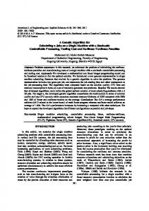
Table 6 (see Appendix B) gives some results including the CPU times of the branch-andbound algorithm, error percentage and number of optimal solutions for heuristic algorithms, the average percentage of fathomed nodes by dominance rules and lower bounds and the average percentage of total fathomed nodes. This table shows that Heu2 and Heu5 have error percentages less than 0.8% and 1.8% respectively, in groups except for the two with T=0.5 and process times between 1 and 100. As it can be seen in Table 5, except for the groups G2, G9, G11 and G12 for 30-job instances, the optimal solutions for all instances are obtained. Figure 2 shows the average percentage of fathomed nodes by lower bounds and dominance rules for 30-job instances. According to this figure, LB1 has the most effect on decreasing the size of the search tree especially for groups with high variation of processing times and penalty weights. This figure shows that except for the four groups G5, G6, G11 and G12, the dominance rule Dom2 performs better than Dom3 because Dom2 is related to tardy jobs and the tardiness factor is 0.8 in these four groups which results in most of the jobs becoming tardy. This figure indicates that LB1 fathoms more nodes in groups with R=0.8 proving that the efficiency of LB1 increases with the increase of due dates variation. The average percentage of fathomed nodes by LB2 is higher in the groups with p   45  55 which is also concluded by Valente [20].

(15)

Average fathomed nodes (%)

70 60 50

DOM1 DOM2

40

DOM3

30

LB1 20

LB2

10 0 G1

G2

G3

G4

G5

G6

G7

G8

G9 G10 G11 G12

Figure 2: Average percentage of fathomed nodes for 30-job instances In Figure 3, the branch-and-bound algorithm running times for groups G1 to G12 are given in a logarithmic scale. According to this figure, the groups G7, G9 and G11 take more computational time compared with the other groups. Among these three groups, G11 has the highest average running times and hence is the most difficult group to be solved optimally. The results show that group G10 is the easiest group with the smallest running times in all problem sizes. The reason may be the overall effect of the two lower bounds. From Figure 2, the overall performance of LB1 and LB2 in G11 is very low, whereas this performance in G10 is higher than in other groups. 10000

running time (s)

1000

30 job

100

25 job 20 job

10

15 job 1 0.1 G1 G2

G3

G4

G5

G6 G7

G8

G9 G10 G11 G12

Figure 3: branch-and-bound running times 5.3. Results of the large-size problems In Table 7, the overall results of the heuristic algorithms for large size instances (50 to 300 jobs) are given. Experiments show that the gap between lower bounds and optimal solutions is considerable in some groups and hence, the error percentages in this table are calculated according to the relative deviation of each answer from the best one obtained from the six heuristics. It can be seen from this table that Heu2 and Heu5 create the best solutions with an average error less than 0.3% for all problem sizes. Also, comparing these two heuristics indicates that Heu2, created from the algorithms 1 and 2, has the best performance in all groups. (16)

Columns "No. best" gives the number of times out of 240 that each heuristic method gives the best solution compared with the other heuristics. According to these columns, heuristic methods Heu2, Heu5 and Heu3 generate the largest number of best solutions, respectively. "CPU time" columns show that the computational effort will increase with increasing problem size. The running times are less than 5 seconds even in large size instances. These low running times indicate that the quality of solutions is the most important factor to show the performance of a method. Table 7: Results of the heuristic methods for large-size problems n

error %

Heu 1 CPU No. time best (s)

Heu 2 error %

Heu 3

CPU No. time best (s)

error %

Heu 4 CPU time (s)

No. best

No. CPU error error % best time (s) %

Heu 5 CPU No. time best (s)

Heu 6 CPU error No. time % best (s)

50

4.0

31

0.00

0.2

181

0.00

2.1

137

0.00

2.6

24

0.00

0.3

177 0.00

2.4

170 0.00

100

4.5

4

0.12

0.1

164

0.30

2.8

118

0.12

2.6

3

0.00

0.2

145 0.42

2.5

150 0.03

150

4.2

1

0.37

0.0

155

0.50

2.7

91

0.38

2.2

2

0.01

0.1

126 0.71

2.1

134 0.18

200

4.4

0

0.52

0.0

144

1.10

3.0

70

0.58

2.0

1

0.02

0.1

121 1.35

1.9

126 0.29

300

0.0

0

1.43

0.0

182

3.60

0.0

114

1.52

1.6

0

0.05

0.0

118 4.25

0.9

0

0.71

Table 8 (see Appendix B) gives some results including heuristic methods' error percentages and number of times out of 20 replications, each heuristic gives the best solution. In Figure 4, the error percentages of the heuristic methods for 200-job instances are plotted on a logarithmic scale. This figure shows that the performance of the methods is higher in groups G7 to G12 in which the variety of processing times and penalty weights is low. According to this figure, two heuristics Heu2 and Heu5 have lower error percentages compared with an other methods while Heu2 seems to have the best performance with the average error less than 0.1% in all groups. 100 10

Average error (%)

1 0.1

Heu1

0.01

Heu2

0.001

Heu3

0.0001

Heu4 Heu5

0.00001

Heu6

0.000001 0.0000001 1E-08 G1

G2

G3

G4

G5

G6

G7

G8

G9 G10 G11 G12

Figure 4: Average error of heuristic algorithms for 200-job instances Figure 5 shows the average error percentage of heuristic algorithms for 300-job instances. According to this figure, the two methods Heu2 and Heu5 have the best results with the smallest error percentages. As in Figure 4, the performance of the methods is higher in groups G7 to G12.

(17)

Average error (%)

Heu Heu Heu Heu Heu Heu

G

G

G

G

G

G

G

G

G

G

G

G

Figure 5: Average error of heuristic algorithms for 300-job instances

6. Conclusion In this paper, a single machine scheduling problem was considered, in which the objective function is to minimize the sum of quadratic earliness and tardiness penalties. In order to develop a branch-and-bound algorithm, some useful bounding procedures and dominance rules were introduced. Some test problems in 12 groups were generated according to different levels of processing times and penalty weights, average tardiness factor, and range of due dates. Computational results demonstrated that the branch-and-bound algorithm is able to solve instances with up to 25 jobs in all the groups and 94% of the 30-job instances. This indicates higher performance of the proposed method compared with the branch-andbound method presented by Valente [20] that is able to solve problems with up to 20 jobs in a reasonable time. The computational results showed that both the upper and lower bounds proposed for the problem are very tight. The lower bound developed based on lagrangian relaxation has a considerable effect on fathoming nodes of the tree because more than 45% of the nodes are fathomed by this lower bound. Among the heuristic methods, the one which is composed of the constructive and improvement algorithms proposed in this paper (Heu2), has the best performance under all problem sizes from 10 to 300 jobs. Experiments indicate that Heu2, with an overall average error less than 1.3%, has a higher performance compared to the method proposed by Valente and Alves [18] (Heu6). We recommend extending this problem to other manufacturing systems such as parallel machines or flow shops as well as considering assumptions like idle insertion and setup times for further research. Although the lower bound proposed in this study performs better than the one developed by Valente and Alves[18], this lower bound is still far from the optimal solution in some instances and it can be improved in future studies.

Acknowledgments The authors are grateful to anonymous referees for helpful comments and suggestions that improved the presentation of the paper. (18)

References [1] Ow PS, Morton TE. Single machine earlt/tardy problem. Management Science. 1989;35:177-91. [2] Valente JMS, Alves RAFS. Improved heuristics for the early/tardy scheduling problem with no idle time. Comput Oper Res. 2005;32:557-69. [3] Valente JMS, Alves RAFS. Filtered and recovering beem search algorithms for thhe early/tardy scheduling problem with no idle time. Comput Ind Eng. 2005;48:363-75. [4] Li G. Single machine earliness and tardiness scheduling. Eur J Oper Res. 1997;96:546-58. [5] Liaw CF. A branch-and-bound algorithm for the single machine earliness and tardiness scheduling problem. Comput Oper Res. 1999;26:679-93. [6] Baker KR, Scudder GD. Sequencing with earliness and tardiness penalties: a review. Operations Research. 1990;38:22-36. [7] Gupta SK, Sen T. Minimizing a quadratic function of job lateness on a single machine. Engineering Costs and Production Economics. 1983;7:187-94. [8] Chung YH, Liu HC, Wu CC, Lee WC. A deteriorating jobs problem with quadratic function of job lateness. Comput Ind Eng. 2009;57(4):1182-6. [9] Su LH, Chang PC. A heuristic to minimize a quadratic function of job lateness on a single machine. Int J Prod Econ. 1998;55(2):169-75. [10] Schaller J. Minimizing the sum of squares lateness on a single machine. Eur J Oper Res. 2002;143(1):64-79. [11] Sen T, Dileepan P, Lind MR. Minimizing a weighted quadratic function of job lateness in the single machine system. Int J Prod Econ. 1996;42(3):237-43. [12] Soroush HM. Single-machine scheduling with inserted idle time to minimise a weighted quadratic function of job lateness. Eur J Ind Eng. 2010;4(2):131-66. [13] Valente JMS. An exact approach for the single machine scheduling problem with linear early and quadratic tardy penalties. Asia Pac J Oper Res. 2008;25(2):169-86. [14] Valente JMS. Heuristics for the single machine scheduling problem with early and quadratic tardy penalties. Eur J Ind Eng. 2007;1(4):431-48. [15] Valente JMS. Beam Search Heuristics for the Single Machine Scheduling Problem with Linear Earliness and Quadratic Tardiness Costs. Asia Pac J Oper Res. 2009;26(3):319-39. [16] Valente JMS, Moreira MRA, Singh A, Alves RAFS. Genetic algorithms for single machine scheduling with quadratic earliness and tardiness costs. Int J Adv Manuf Tech. 2011;54(1-4):251-65. [17] Schaller J. Single machine scheduling with early and quadratic tardy penalties. Comput Ind Eng. 2004;46(3):511-32. [18] Valente JMS, Alves RAFS. Heuristics for the single machine scheduling problem with quadratic earliness and tardiness penalties. Comput Oper Res. 2008;35(11):3696-713. [19] Valente JMS, Moreira MRA. Greedy randomised dispatching heuristics for the single machine scheduling problem with quadratic earliness and tardiness penalties. Int J Adv Manuf Tech. 2009;44(9-10):995-1009. [20] Valente JMS. An exact approach for single machine scheduling with quadratic earliness and tardiness penalties. Porto: Faculdade De Economia, Universidade Do Porto; 2007. [21] Valente JMS. Beam search heuristics for quadratic earliness and tardiness scheduling. J Oper Res Soc. 2010;61(4):620-31. [22] Xia Y, Chen BT, Yue JF. Sequence jobs and assign due dates with uncertain processing times and quadratic penalty functions. Lect Notes Comput Sc. 2005;3521:261-9. [23] Szwarc W, Mukhopadhyay SK. Minimizing a Quadratic Cost Function of Waiting-Times in Single-Machine Scheduling. J Oper Res Soc. 1995;46(6):753-61. [24] Mittenthal J, Raghavachari M. Stochastic Single-Machine Scheduling with Quadratic EarlyTardy Penalties. Operations Research. 1993;41(4):786-96. [25] Kubiak W. New Results on the Completion-Time Variance Minimization. Discrete Appl Math. 1995;58(2):157-68. [26] Kahlbacher HG, Cheng TCE. Processing-Plus-Wait Due-Dates in Single-Machine Scheduling. J Optimiz Theory App. 1995;85(1):163-86. [27] Cheng TCE, Liu Z. Parallel machine scheduling to minimize the sum of quadratic completion times. Iie Trans. 2004;36(1):11-17. (19)

[28] Wei CM, Wang JB. Single machine quadratic penalty function scheduling with deteriorating jobs and group technology. Appl Math Model. 2010;34(11):3642-7. [29] Mondal SA, Sen AK. An improved precedence rule for single machine sequencing problems with quadratic penalty. Eur J Oper Res. 2000;125(2):425-8. [30] Dellacroce F, Szwarc W, Tadei R, Baracco P, Ditullio R. Minimizing the Weighted Sum of Quadratic Completion Times on a Single-Machine. Naval Research Logistics. 1995;42(8):1263-70. [31] Nawaz M, Enscore JR, Ham EE. A heuristic algorithm for the m-machine n-job flow-shop sequencing problem. OMEGA International Journal of Management Science. 1983;11:91-5.

Appendix A: Lemma 1: Noting that E i (t ) and T j t  are continuous functions, any linear combination of them is also continuous. The functions E i (t ) and T i (t ) are respectively decreasing and increasing and according to the fact that the sum of some increasing (decreasing) functions is also increasing (decreasing), we can conclude that F (t ) is a decreasing function. It is obvious that lim F (t )   and lim F (t )   and considering F (t ) as a continuous function, it can be t 

t 

concluded that t * | F (t * )  0 .

□

Theorem 1: The function Z t    Nj 1  h j E j2 t  w jT j2 t   is the sum of continuous functions (earliness and tardiness penalties) and hence a continuous function. Consider a set of adjacent and fixed-ordered jobs    where t indicates the start time of the first job in this set. If the sets of early, tardy and on-time jobs in this set are denoted by G E (t ) , GT (t ) and GO (t ) , respectively, then according to Lemma 1, the term F (t )  i G (t )  hi E i (t )    j G (t ) w jT j (t )  E

T

is a continuous and decreasing function and hence, there is a value t  t satisfying F (t * )  0 . For each t1  t * we have *

Z t1   i G

E

t1 

h E    i

2 i

j GT t1 

w T  j

2 j

Define the "cost breakdown point" as the cut-off point defined per job that a completion time related to a job in set  conflicts with the due date of that job. If the set  is shifted to the end of sequence by  points ( t  t   ) such that no cost breakdown point is met, then Z t1     i G

E t1 

h E i



     j G 2

i

T

t1 

w

j

T

j

 

2



And so, Z t 1     Z t 1    i G

E

t 1 

 h 

 2E i 

  

h     Z  t     Z t    h    

 Z t 1     Z t 1    i G 

2

i

t 1 

i

w w  

1

i G E t1

i

j

2

 2T j 





j

 2   2

j GT t1

j

 2   2 F t 1   0

2

1

w 

j GT t1 

2

E

j GT t1 

i G E t1 

 h E t     i

i

1

j GT t1 

w T t    j

j

1

 Z t 1     Z  t 1 

Suppose that t1 is a start point of the set  related to one of the cost breakdown points, hence the following equations will hold. Z t1     i G

E t1 

h E i



     j G 2

i

T t1 

w

(20)

j

T



     j G 2

j

O

t1 

w

j

2

Z t 1     Z t 1    i G

E

t 1 

 h 

 Z t 1     Z t 1    i G

2

i

 2E i 

  

h     2

E

t 1 

i

j GT t1 

j GT t1 

w

j

w  j

2

 2T j 

  

 2   2 F t 1    k G

O

w   w  0   2

k GO t1 

k

2

t1

k

 Z t 1     Z t 1 

We proved that the function Z (t ) is increasing on the right hand side of the point t  t * . By the same way, it can be proved that Z (t ) is decreasing on the left hand side of this point such as t 2  t * . This will complete the proof. □ Theorem 2: The theorem is easily proved by contradiction. Suppose that the theorem does not hold, thus one of the following conditions will occur. 1 j   :  j   j and  j 1   j 1 2 j   :  j   j and  j 1   j 1

According to the first group of constraints from dual problem D1, we have:  j  j 1 3  p j p j 1 and based on the definition of set   j  j 1 4  p j p j 1 So, it can be shown that condition 1 does not hold as follows.     1 3 1 , 4   j  j 1  j  j 1  contradiction p j p j 1 p j p j 1 The same conclusion is made for condition 2 .

□

Theorem 3: Let j 1 and j 2 be two jobs in sub-set  1 , respectively. Then, the relations

j

1

p j1



j

1

p j1  j1 p j1

j

2

p j2 

,

 j2 p j2

 

j

1

p j1   j2 p j2



j

2

p j2

and  j 2   j 2 hold. 

  0

 j2 j   j 2  j 2    2    Min p j1      Min  j1   j1  Min p j1 p j2 p j2  0  

Since  is a non-negative constant, the minimum value of the above relation is achieved by setting   0 . The same conclusion can be made for any two jobs in  2 or  3 . Also, using the above procedure we can prove that the  p ratios for any two jobs in different sub-sets are the same, and this completes the proof. Theorem 4: The proof is done by contradiction. Suppose that  2 is empty and   is optimal for set  that is not equal to any  p ratios.     Min  i  i  Min     . p j   j      j     . p j    Min   p j   p j   .  j  j  j i   j :  j    j :   j :   j :   pj p j p j  pj 

(21)

It is obvious that if the expression in brackets is positive then reducing   will improve the minimization objective and if the expression in parenthesis is negative then increasing   will improve it. □ Theorem 5: Suppose the current solution is not optimal and reducing   improves the dual objective function. Then we have, Min   i  i  Min i 

 Min

   .p

j 1

j

 j  

 

j 1

 

j  2

j

j

 j  

 

j  2

   .p j   

j

 j

 

j  3

j 

 

j  3

j 

  j  

   . p j  

   Min   .    p j     p j      p j     cte j  2 j  3  j 1 

According to the first equation of this theorem, the term in brackets is always non-positive and so, reducing   will not improve the objective function. Again, suppose that the current solution is not optimal and increasing   improves the dual objective function. So, Min   i  i  Min i 

 Min

   .p

j 1

j

 j  

 

j 1

j

   .p

j  2

 j   j

 

j  2

 j  

j

 j 

 

j  3

j 

 

j  3

j 

  j  

   . p j  

   Min   .    p j     p j      p j     cte j  2 j  3  j 1 

According to the second equation of this theorem, the term in brackets is always nonnegative and so, increasing   will not improve the objective function. □ Theorem 6: In this algorithm, all the jobs from the last to the first are grouped according to Definition 1. We know from Theorem 3 that all jobs in a group have the same  p (denoted by   ) and thus, it is sufficient to determine the value of   for each group of jobs. On the other hand, the sub-set  2 is nonempty in each group and thus,   is equal to the proportion

 p related to one of the jobs in set  . In order to be optimal, the value of   should satisfy Theorem 5. In step 2, each   is set greater than or equal to its value in the optimal solution of D1 . In step 4, the algorithm checks whether a group Sk meets the conditions in Theorem 5; if the conditions hold, then the algorithm goes to the previous group; otherwise the value of  k is tuned such that the conditions of Theorem 5 are met. In step 5, the algorithm will merge two adjacent groups if their  values conflict. Step 6 calculates the optimal values of the lagrangian multipliers using the processing times and  values obtained from the previous steps. □

(22)

Appendix B: Table 6: Average error of heuristic algorithms for 10-30 job instances n

G

10 G1 G2 G3 G4 G5 G6 G7 G8 G9 G10 G11 G12

15 G1 G2 G3 G4 G5 G6 G7 G8 G9 G10 G11 G12

20 G1 G2 G3 G4 G5 G6 G7 G8 G9 G10 G11 G12

25 G1 G2 G3 G4 G5 G6 G7 G8 G9 G10 G11 G12

30 G1 G2 G3 G4 G5 G6 G7 G8 G9 G10 G11 G12

B&B No. Ave. Solved CPU (s)

Heu 1 error No. % Opt

Heu 2 error No. % Opt

Heu 3 error No. % Opt

Heu 4 No. error % Opt

Total Heu 5 Heu 6 Percentage of fathomed nodes by fathomed error No. error No. Dom Dom Dom % Opt % Opt 1 2 3 LB 1 LB 2 nodes (%)

20 20 20 20 20 20 20 20 20 20 20 20

0.1 0.0 0.0 0.1 0.0 0.1 0.1 0.1 0.1 0.1 0.1 0.1

5.2 7.4 12.3 18.0 3.5 0.7 0.0 0.0 0.0 0.0 0.0 0.0

4 6 8 9 14 14 20 20 20 20 18 20

0.0 0.8 0.7 4.4 0.5 0.0 0.0 0.0 0.0 0.0 0.0 0.0

19 0.0 15 0.8 18 4.8 15 16.0 19 1.3 20 0.0 20 0.0 20 0.0 20 0.0 20 0.0 19 0.0 20 0.0

20 17 17 16 17 20 20 20 20 20 19 20

88.3 108.3 228.9 297.2 20.3 22.0 0.8 0.5 1.7 1.1 0.8 0.5

0 0 0 0 1 2 2 7 1 9 2 8

0.3 1.8 3.8 2.9 0.3 0.1 0.0 0.0 0.0 0.0 0.0 0.0

16 15 11 15 16 18 20 20 20 20 20 20

8.8 11.8 44.5 8.1 2.1 0.2 0.0 0.0 0.0 0.0 0.0 0.0

11 10 7 15 15 19 20 20 20 20 19 20

0.8 0.3 0.6 3.1 4.2 7.8 0.0 0.1 3.7 4.2 27.9 23.3

16.9 20.2 24.1 8.4 7.9 4.3 19.9 15.3 10.7 2.6 0.8 0.0

6.2 7.0 14.6 15.0 20.9 20.1 0.0 0.3 8.1 6.5 15.2 2.1

71.4 69.9 59.8 72.8 67.0 67.8 52.4 69.9 50.4 71.5 55.0 69.5

4.7 2.6 0.9 0.7 0.0 0.0 27.7 14.4 27.1 15.2 1.1 5.1

82.2 83.0 84.2 83.5 83.9 83.9 84.9 83.9 83.2 83.3 84.7 84.3

20 20 20 20 20 20 20 20 20 20 20 20

0.2 0.5 0.5 0.5 0.3 0.5 0.5 0.2 0.7 0.2 1.2 0.9

5.4 3.9 23.9 12.0 0.5 0.8 0.0 0.0 0.0 0.0 0.0 0.0

0 1 4 4 13 8 11 19 17 20 17 17

0.4 0.2 3.7 2.0 0.1 0.3 0.0 0.0 0.0 0.0 0.0 0.0

14 0.4 13 1.5 10 15.9 16 3.5 17 0.1 18 0.3 19 0.0 20 0.0 20 0.0 20 0.0 20 0.0 20 0.0

17 15 6 16 16 18 19 20 20 20 19 20

76.8 106.1 315.2 477.2 25.7 50.7 1.1 1.0 2.7 4.1 0.7 0.4

0 0 0 0 0 0 0 2 0 3 0 2

0.1 0.4 3.1 4.4 0.1 0.3 0.0 0.0 0.0 0.1 0.0 0.0

16 11 7 9 14 17 19 20 20 19 19 20

25.5 21.1 75.0 46.2 1.7 1.5 0.0 0.0 0.0 0.0 0.0 0.0

3 7 0 5 7 12 17 20 20 20 16 20

0.2 0.3 1.0 1.2 5.7 11.6 0.0 0.0 3.2 2.0 29.4 25.1

26.0 29.3 36.8 19.9 12.0 9.2 29.6 21.9 17.6 4.7 1.9 1.1

2.6 6.9 13.4 17.2 28.5 22.4 0.0 0.1 10.0 5.7 15.9 7.0

69.1 61.2 48.4 60.5 53.8 56.7 44.4 69.2 42.2 69.3 52.6 64.5

2.1 2.3 0.4 1.2 0.0 0.0 26.0 8.8 26.9 18.2 0.2 2.3

88.9 88.6 89.7 88.8 89.5 89.6 90.6 90.0 89.2 88.8 90.5 89.9

20 20 20 20 20 20 20 20 20 20 20 20

1.7 7.5 3.7 5.7 2.3 4.3 7.4 2.0 5.4 0.6 19.8 5.3

9.9 5.4 16.7 30.2 1.9 2.2 0.0 0.0 0.0 0.0 0.0 0.0

0 0 0 1 3 6 16 20 16 19 16 18

0.1 0.3 9.9 5.5 0.1 0.0 0.0 0.0 0.0 0.0 0.0 0.0

13 0.2 12 0.4 2 13.4 9 20.8 11 1.3 19 0.7 20 0.0 20 0.0 20 0.0 20 0.0 19 0.0 20 0.0

14 14 0 9 12 17 20 20 20 20 19 20

83.4 99.8 447.4 752.4 30.5 44.7 0.8 0.6 3.6 5.3 0.6 0.5

0 0 0 0 0 0 0 0 0 0 0 1

0.2 0.4 5.2 6.7 0.3 0.1 0.0 0.0 0.0 0.0 0.0 0.0

11 33.0 0 13 29.5 0 7 161.4 0 10 122.9 1 12 3.0 4 15 5.5 7 20 0.0 18 20 0.0 20 19 0.1 16 20 0.0 20 17 0.0 17 20 0.0 20

0.2 0.1 0.4 1.0 5.0 8.9 0.0 0.0 2.2 1.0 26.1 21.5

37.2 36.5 44.7 22.9 19.8 13.8 42.5 25.1 22.4 7.9 5.4 1.9

1.6 7.4 11.5 15.7 32.7 27.0 0.0 0.0 7.3 4.5 25.5 8.9

60.3 54.4 43.1 59.2 42.4 50.2 38.0 68.4 32.6 68.4 42.7 66.4

0.8 1.6 0.3 1.2 0.0 0.0 19.4 6.5 35.4 18.2 0.3 1.3

92.0 91.1 92.3 91.7 92.6 92.2 93.1 92.8 92.0 92.2 92.9 92.7

20 20 20 20 20 20 20 20 20 20 20 20

8.8 42.6 26.1 43.6 17.2 69.5 136.8 20.3 78.4 4.0 365.2 63.0

4.5 5.7 31.1 19.3 0.6 1.2 0.0 0.0 0.0 0.0 0.0 0.0

0 0 0 3 1 2 14 16 16 20 13 13

0.1 0.0 4.0 2.5 0.1 0.0 0.0 0.0 0.0 0.0 0.0 0.0

9 0.1 14 0.3 9 20.3 11 10.7 14 0.3 16 0.4 19 0.0 20 0.0 20 0.0 20 0.0 20 0.0 20 0.0

13 15 3 9 11 12 20 20 20 20 20 20

70.7 113.2 458.5 984.7 27.3 39.9 1.0 0.7 3.5 11.3 0.7 0.5

0 0.2 11 27.9 0 0 0.1 13 35.9 1 0 2.0 4 186.4 0 0 12.6 3 177.8 0 0 0.1 13 5.5 0 0 0.2 11 3.2 2 0 0.0 19 0.0 15 0 0.0 20 0.0 19 0 0.0 17 0.1 16 0 0.0 20 0.0 19 0 0.0 18 0.0 10 0 0.0 20 0.0 19

0.0 0.0 0.2 1.0 3.7 8.3 0.0 0.0 2.1 1.0 25.4 24.8

41.4 45.1 48.5 20.7 27.6 16.9 45.0 28.0 25.9 7.7 7.4 1.8

1.2 7.3 8.6 18.3 35.3 36.9 0.0 0.0 9.5 5.2 30.5 11.0

57.1 46.3 42.5 59.0 33.5 37.8 34.6 69.3 27.7 71.1 36.7 61.9

0.2 1.3 0.2 1.1 0.0 0.0 20.4 2.8 34.7 15.1 0.0 0.6

93.8 92.6 94.2 93.3 94.1 93.9 94.6 94.3 93.5 94.0 94.4 94.3

20 102.3 18 457.8 20 238.9 20 329.2 20 67.6 20 252.7 20 1247.9 20 101.4 19 612.1 20 15.0 10 2452.0 19 482.8

3.4 8.7 27.4 18.5 4.1 0.8 0.0 0.0 0.0 0.0 0.0 0.0

0 0 0 1 1 3 10 14 13 17 5 16

0.1 0.7 2.2 4.7 0.0 0.0 0.0 0.0 0.0 0.0 0.0 0.0

8 0.2 9 1.6 4 20.5 7 7.6 15 2.1 12 0.2 19 0.0 20 0.0 17 0.0 19 0.0 9 0.0 19 0.0

5 66.3 6 129.5 3 511.4 4 1211.1 8 37.2 15 33.7 20 0.9 20 0.8 17 3.5 20 11.0 10 0.9 19 0.4

0 0.3 8 30.2 0 0 0.1 9 52.5 0 0 7.9 3 238.3 0 0 11.3 3 261.7 0 0 0.2 10 9.0 0 0 0.0 14 2.7 2 0 0.0 18 0.1 9 0 0.0 20 0.0 16 0 0.0 15 0.2 8 0 0.0 19 0.0 18 0 0.0 10 0.1 3 0 0.0 19 0.0 19

0.1 0.0 0.3 0.9 4.3 8.5 0.0 0.0 1.1 0.7 18.1 22.9

44.9 45.7 54.5 24.2 28.6 19.6 49.8 29.3 29.5 9.9 11.3 3.0

1.0 8.4 9.8 16.9 33.7 33.1 0.0 0.0 8.2 5.3 32.3 13.2

53.7 44.7 35.3 57.0 33.4 38.9 30.5 67.9 25.8 67.3 38.3 60.5

0.3 1.1 0.1 0.9 0.0 0.0 19.6 2.8 35.4 16.7 0.0 0.3

94.9 93.6 95.1 94.4 95.1 94.9 95.5 95.3 94.7 95.1 95.5 95.1

(23)

Table 8: Average error of heuristic algorithms for 50-300 job instances

50

G1 G2 G3 G4 G5 G6 G7 G8 G9 G10 G11 G12

Heu 1 No. error % Opt 2.73 0 3.84 0 25.29 0 12.98 0 2.86 0 0.44 0 0.01 1 0.00 7 0.01 4 0.00 14 0.01 0 0.00 5

100

G1 G2 G3 G4 G5 G6 G7 G8 G9 G10 G11 G12

2.89 5.18 27.28 14.23 3.90 0.43 0.01 0.00 0.01 0.00 0.01 0.00

0 0 0 0 0 0 0 0 1 2 0 1

0.03 0.01 0.38 0.17 0.01 0.00 0.00 0.00 0.00 0.00 0.00 0.00

11 9 14 13 11 4 16 19 15 18 18 16

1.19 2.41 19.88 7.04 3.29 0.08 0.00 0.00 0.00 0.00 0.00 0.00

0 0 0 0 9 5 15 20 17 19 15 18

0.09 0.02 19.50 7.88 3.92 0.02 0.00 0.00 0.00 0.00 0.00 0.00

0 0 0 0 0 0 0 2 0 1 0 0

0.01 0.01 1.62 0.58 0.03 0.00 0.00 0.00 0.00 0.00 0.00 0.00

13 8 6 8 8 8 12 16 14 17 17 18

0.07 0.01 18.50 7.15 3.86 0.01 0.00 0.00 0.00 0.00 0.00 0.00

12 16 0 0 7 11 15 20 18 19 15 17

150

G1 G2 G3 G4 G5 G6 G7 G8 G9 G10 G11 G12

3.16 4.41 23.51 15.95 2.98 0.39 0.01 0.00 0.01 0.00 0.01 0.00

0 0 0 0 0 0 0 0 0 1 0 0

0.04 0.00 0.28 0.04 0.00 0.00 0.00 0.00 0.00 0.00 0.00 0.00

7 9 13 17 12 5 11 16 15 20 12 18

1.74 2.55 17.33 8.73 2.49 0.06 0.00 0.00 0.00 0.00 0.00 0.00

0 0 0 0 4 3 9 20 13 20 6 16

0.02 0.01 16.62 6.27 3.21 0.01 0.00 0.00 0.00 0.00 0.00 0.00

0 0 0 0 0 0 0 2 0 0 0 0

0.00 0.00 1.16 0.59 0.03 0.00 0.00 0.00 0.00 0.00 0.00 0.00

9 5 7 2 9 7 10 15 13 17 15 17

0.02 0.00 16.11 5.96 2.98 0.00 0.00 0.00 0.00 0.00 0.00 0.00

8 12 0 1 5 10 19 20 15 19 11 14

200

G1 G2 G3 G4 G5 G6 G7 G8 G9 G10 G11 G12

3.51 5.50 24.88 14.65 3.97 0.47 0.01 0.00 0.01 0.00 0.01 0.00

0 0 0 0 0 0 0 0 0 0 0 0

0.01 0.00 0.09 0.05 0.00 0.00 0.00 0.00 0.00 0.00 0.00 0.00

11 7 17 12 11 4 11 16 7 17 13 18

2.21 3.69 18.00 8.38 3.48 0.08 0.00 0.00 0.00 0.00 0.00 0.00

0 0 0 0 2 0 3 18 11 20 7 9

0.04 0.01 13.21 6.58 3.95 0.01 0.00 0.00 0.00 0.00 0.00 0.00

0 0 0 0 0 0 1 0 0 0 0 0

0.01 0.00 0.88 0.51 0.04 0.00 0.00 0.00 0.00 0.00 0.00 0.00

8 3 3 5 6 10 5 16 10 17 19 19

0.03 0.00 13.01 6.37 3.78 0.01 0.00 0.00 0.00 0.00 0.00 0.00

7 14 0 3 5 8 12 19 16 20 13 9

300

G1 G2 G3 G4 G5 G6 G7 G8 G9 G10 G11 G12

3.20 5.26 23.54 15.82 4.38 0.45 0.01 0.00 0.01 0.00 0.01 0.00

0 0 0 0 0 0 0 0 0 0 0 0

0.01 0.00 0.03 0.00 0.02 0.00 0.00 0.00 0.00 0.00 0.00 0.00

14 14 19 19 6 10 11 19 7 14 5 16

2.33 3.97 18.21 10.23 3.72 0.06 0.00 0.00 0.00 0.00 0.00 0.00

0 0 0 0 1 0 1 15 6 19 2 10

30.69 65.98 407.74 690.87 15.44 26.50 0.00 0.00 0.00 0.00 0.00 0.00

0 0 0 0 0 0 0 0 0 0 0 0

0.02 0.00 2.17 1.72 0.01 0.00 0.00 0.00 0.00 0.00 0.00 0.00

11 9 1 1 14 12 2 16 8 13 17 16

26.39 56.61 374.48 593.80 13.25 20.05 0.00 0.00 0.00 0.00 0.00 0.00

0 0 0 0 0 0 0 0 0 0 0 0

n

G

Heu 2 No. error % Opt 0.05 11 0.02 12 1.51 9 0.39 9 0.01 15 0.01 12 0.00 18 0.00 20 0.00 19 0.00 18 0.00 19 0.00 19

Heu 3 No. error % Opt 0.60 0 0.73 0 17.96 0 4.24 2 2.11 10 0.07 14 0.00 18 0.00 20 0.00 17 0.00 19 0.00 18 0.00 19

Heu 4 No. error % Opt 0.10 0 0.04 0 17.76 0 9.40 0 3.92 0 0.10 0 0.00 1 0.00 8 0.01 2 0.00 5 0.00 3 0.00 5

Heu 5 No. error % Opt 0.02 11 0.00 13 1.14 12 1.92 10 0.02 15 0.00 13 0.00 11 0.00 19 0.00 15 0.00 18 0.00 20 0.00 20

Heu 6 No. error % Opt 0.04 12 0.00 19 17.09 0 8.14 5 3.88 12 0.05 16 0.00 15 0.00 20 0.00 14 0.00 19 0.00 19 0.00 19

(24)