In: Scientific Computing, Validated Numerics, Interval Methods, W. Kramer and J.W.von Gudenberg (Eds.), Kluwer Academic Publishers, New York, pp. 215-226, 2001.
A BRANCH-AND-PRUNE METHOD FOR GLOBAL OPTIMIZATION The Univariate Case D.G. Sotiropoulos and T.N. Grapsa University of Patras, Department of Mathematics GR-265 00 Rio, Patras, Greece.
[email protected],
[email protected]
Keywords: Global optimization, interval arithmetic, optimal center, branch and prune. Abstract
1.
We present a branch-and-prune algorithm for univariate optimization. Pruning is achieved by using first order information of the objective function by means of an interval evaluation of the derivative over the current interval. First order information aids fourfold. Firstly, to check monotonicity. Secondly, to determine optimal centers which, along with the mean value form, are used to improve the enclosure of the function range. Thirdly, to prune the search interval using the current upper bound of the global minimum, and finally, to apply a more sophisticated splitting strategy. Results of numerical experiments are also presented.
INTRODUCTION
Let f : D → IR be a C 1 function, where D is the closure of a nonempty bounded open subset of IR. We assume that for an interval X ⊆ D an interval arithmetic evaluation of its derivative exists. Our underlying problem can be formulated as follows: Given a compact interval X ⊆ D, find the global minimum f ∗ = min f (x) x∈X
(1.1)
and the set of all global minimum points X ∗ = {x ∈ X : f (x) = f ∗ }. Interval arithmetic is extensively studied in [9]. For what follows, we need some notions and notations. Let II = {[a, b] | a ≤ b, a, b ∈ IR} be the set of compact intervals. Let also x be the lower endpoint and x be
1
2 the upper endpoint of an interval X. If X = [x, x] is a given interval, we denote by mid(X) = (x+x)/2 the midpoint and rad(X) = (x−x)/2 the radius of X. Let frg (X) = {f (x) : x ∈ X} be the range of f over X. A function F : II → II is called an inclusion function for f if frg (X) ⊆ F (X) for any X ∈ II. The inclusion function of the derivative of f is denoted by F 0 . Inclusion functions can be produced in a number of ways such as natural extension, mean value forms, and Taylor expansion. Each of these forms has slightly different properties and convergence order. For a more thorough discussion on these issues, see [11]. In this work we present an interval branch-and-prune algorithm based on the branch-and-bound principle [7, 8, 12]. The algorithm uses a new accelerating device, called derivative pruning step. This accelerating device uses first order information and its geometric interpretation is similar to slope pruning given by Ratz in [13]. Moreover, the optimal center of a mean-value form with respect to the lower bound is used to define a new subdivision strategy. The numerical results indicate that the use of the optimal center leads to more efficient interval algorithms for global optimization. The rest of the paper is organized as follows. In Section 2 we present the way we determine an optimal center in mean-value forms and give some valuable properties. We next describe the derivative pruning step and define our subdivision strategy, while in Section 4 we present our model algorithm. We evaluate the proposed subdivision strategy and compare it with a variant of our algorithm that uses bisection in Section 5. Numerical results for a complete test set are also reported.
2.
OPTIMAL CENTERS AND MEAN-VALUE FORMS
A way for reducing overestimation in the evaluation of a differentiable function f ∈ C 1 is the use of a standard tool in interval analysis, the Mean Value Theorem [9]: f (x) − f (c) ∈ F 0 (X) · (x − c), for all x, c ∈ X,
(1.2)
where F 0 (X) is an interval extension of the derivative of f . Then, the interval function Fm : II → II defined as Fm (X, c) = f (c) + F 0 (X) · (X − c), for c ∈ X,
(1.3)
is called mean-value form of f on X with center c. It was shown in [2] that the mean-value form is inclusion isotone and when X is narrow, it often provides tighter enclosures than the natural extension of f . As relation (1.3) shows, to bound f it suffices to bound another function f 0 .
A Branch-and-Prune Method for Global Optimization
3
The following theorem states the main result for the quadratic convergence of mean-value form to frg (X), i.e., w (Fm (X, c)) − w (frg (X)) = O(w(X)2 ). A proof can be found in [11, pp. 71]. Theorem 1 (Krawczyk-Nickel) Let f : D ⊆ IR → IR and let F 0 be an inclusion function for f 0 . Then, the mean-value form (1.3) is quadratically convergent if the estimation F 0 satisfies a Lipschitz condition. In general, the center c in the mean-value form (1.3) is chosen to be the midpoint of the interval X. However, Baumann in [1] introduced the notion of the “optimal” center of a mean-value form and proved that, given the optimal center, the lower bound of the mean-value form has the greatest value among all other possible centers within a given interval. In this paper, we study the opposite direction: We determine the center for which the lower bound of the mean-value form attains its maximum and prove that this point is identical to the optimal center defined by Baumann [1]. We next give some formal definitions and state some theoretical results. Definition 1 The mean-value form (1.3) is called optimal with respect to the lower bound if inf Fm (X, c) ≤ inf Fm (X, c∗ ), for any c ∈ X, while the point c∗ which yields the greatest lower bound among all centers is called optimal center. Theorem 2 Let f : D → IR be a C 1 function, X = [x, x] ∈ II and F 0 (X) = [d, d] be an enclosure of the derivative of f over X. Then, the lower bound of the mean-value form attains its maximum at the center
x, , x c∗ = d+d , mid(X) − rad(X) · d−d
if d ≤ 0, if d ≥ 0, if d < 0 < d.
To prove Theorem 2 we need the following lemma: Lemma 1 Let X ∈ II be a closed interval and ψ1 , . . . ψm : X → IR be affine functions. Then, the function φ(x) = min1≤i≤m ψi (x), x ∈ X, is piecewise linear and concave. Proof: By definition, φ(x) is piecewise linear, that is, a nonsmooth function. To prove concavity, notice that every affine function is convex as
4 well as concave. Thus, φ (λx1 + (1 − λ)x2 ) =
min ψi (λx1 + (1 − λ)x2 )
1≤i≤m
≥ λ min ψi (x1 ) + (1 − λ) min ψi (x2 ) 1≤i≤m
1≤i≤m
= λφ(x1 ) + (1 − λ)φ(x2 ), for every λ ∈ IR, 0 ≤ λ ≤ 1, and every x1 , x2 ∈ X. Theorem 3 If φ is concave on a closed interval X ∈ II with a local maximum at x∗ ∈ X, then φ has a global maximum at x∗ . Proof: See [3, page 267] for a proof. Proof of Theorem 2: We firstly consider the case where d < 0 < d. By applying the interval multiplication rules, it is easy to see that the infimum of relation (1.3) takes the form o
n
inf Fm (X, c) = f (c) + min d · (x − c), d · (x − c)
(1.4)
To determine the point c which yields the greatest lower bound of (1.3), it suffices to solve the following simple max-min problem: max φ(c), c∈X
φ(c) = min ψi (c), 1≤i≤2
(1.5)
c ∈ X,
where ψ1 (c) = −d · c + d · x and ψ2 (c) = −d · c + d · x are both affine functions. According to Lemma 1, φ is a piecewise linear and concave function. This, combined with Theorem 3, implies that any local maximum of φ is also a global maximum. The graphs of ψ1 , ψ2 , and φ are depicted in figure 1. Since d < 0 < d, ψ1 (c) is a strictly monotone increasing function while ψ2 (c) is strictly monotone decreasing one. The slope of the extreme left-hand linear piece equals −d > 0 while the slope of the extreme right-hand linear piece equals −d < 0. Notice that the slope changes only at the point c∗ where φ(c) attains the global maximum. In this case the point c∗ is determined as the intersection point of the affine functions ψ1 and ψ2 : ψ1 (c∗ ) = ψ2 (c∗ ) ⇒ c∗ = mid(X) − rad(X) ·
d+d , d−d
(1.6)
where the endpoints x and x have been substituted by mid(X) − rad(X) and mid(X) + rad(X), respectively.
A Branch-and-Prune Method for Global Optimization
Figure 1
5
Graphical presentation of functions ψ1 , ψ2 and φ when d < 0 < d.
For the remaining cases, when d ≤ 0, φ(c) attains the global maximum at the right endpoint x while φ(c) attains the global maximum at the left endpoint x when d ≥ 0. Relation (1.3) along with Theorem 2 establishes the following lemma: Lemma 2 Let c∗ ∈ X be the optimal center with respect to the lower bound of the mean-value form. Then,
f (c∗ ) + w(X) · d , f (c∗ ) − w(X) · d , inf Fm (X, c∗ ) = d·d ∗ , f (c ) + w(X) · d−d
if d ≤ 0, if d ≥ 0, if d < 0 < d.
Theorem 4 Let f : D → IR be a C 1 function, X = [x, x] ∈ II and F 0 (X) = [d, d] be an enclosure of the derivative of f over X. Then, the upper bound of the mean-value form attains its minimum at the center
x, x, c∗ = d + d , mid(X) + rad(X) · d−d
if d ≤ 0, if d ≥ 0, if d < 0 < d.
Proof: The proof is analogous to the proof of Theorem 2. Remark. It is worthy to notice that when 0 ∈ F 0 (X), the points c∗ and c∗ are symmetric with respect to the midpoint of the interval X. Moreover, their position within a given interval X depends only on the sign of the sum d + d, since the denominator d − d is always positive. Specifically, (a) If d + d > 0 , then c∗ < mid(X) < c∗ . (b) If d + d < 0 , then c∗ < mid(X) < c∗ . (c) If d + d = 0 , then c∗ ≡ mid(X) ≡ c∗ .
6 Neumaier has pointed out that a better enclosure for the range can be obtained by using bicentered forms [10, pp. 59]. This improvement is achieved by intersecting the mean value forms with centers c∗ and c∗ . The price to pay for this improvement is an extra function evaluation at the point c∗ . In our problem, however, the upper bound of the mean value form is of no interest, since a better upper bound f˜ for the global minimum can be obtained by evaluating the function at any point. It was shown in [2] that the mean-value form is inclusion isotone. A weaker property that holds for all optimal mean-value forms has been introduced in [1]: Definition 2 An interval function F : II → II will be called one-sided isotone if one of the following conditions is fulfilled for all X, Y ∈ II: X ⊆ Y implies inf F (X) ≥ inf F (Y ) (lower bound isotonicity) X ⊆ Y implies sup F (X) ≤ sup F (Y ) (upper bound isotonicity) One-sided isotonicity requires only that at least one bound is improved over smaller intervals while inclusion isotonicity implies that both lower and upper bound isotonicity are improved simultaneously.
3.
PRUNING THE SEARCH INTERVAL
In [5], Hansen and Sengupta have determined the feasible region for an inequality constrained problem by solving a set of interval linear inequalities. Inspired by their work, we have developed a process for iteratively pruning the search interval. This pruning technique is based on first-order information and serves as an accelerating device in our algorithm. After reading this section, the reader can see that this is an alternative view of the slope pruning step given in [13] when applied to differentiable functions. Let f˜ denote the smallest currently known upper bound of f ∗ . Taking into account that f ∈ C 1 , the bound f˜ can be used in an attempt to prune the current subinterval X. We would like to find an interval enclosure Y of the set of points y for which f (y) ≤ f˜. Expanding f about the optimal center c = c∗ ∈ X, we obtain f (y) = f (c) + (y − c) · f 0 (ξ), where ξ is a point between c and y. Since c ∈ X and y ∈ X, then ξ ∈ X. Thus, f (y) ∈ f (c) + F 0 (X) · (y − c) ≤ f˜. Let z = y − c, fc = f (c) and D = F 0 (X). Then, the interval inequality becomes: ³ ´ fc − f˜ + D · z ≤ 0. (1.7)
7
A Branch-and-Prune Method for Global Optimization
The solution set Z of the above inequality is determined as follows (see, [5],[6]):
Z=
[−∞, (f˜ − fc )/d] ∪ [(f˜ − fc )/d, +∞] , [−∞, (f˜ − fc )/d] , ˜
[(f − fc )/d, +∞] ∅ [−∞, +∞] [−∞, (f˜ − fc )/d] [(f˜ − fc )/d, +∞]
, , , , ,
if if if if if if if
f˜ < fc , f˜ < fc , f˜ < fc , f˜ < fc , f˜ ≥ fc , f˜ ≥ fc , f˜ ≥ fc ,
d < 0 < d, d ≥ 0 and d > 0, d < 0 and d ≤ 0, d = d = 0, d ≤ 0 ≤ d, d > 0, d < 0.
(α) (β) (γ) (δ) (ε) (ζ) (η)
Recall that z = y − c; therefore the set Y of points y ∈ X that satisfy (1.7) is Y = c + Z. Since we are only interested in points y ∈ X, we compute the interval enclosure Y as Y = (c + Z) ∩ X.
(1.8)
Cases (ζ) and (η) cannot occur due to monotonicity test. Thus, the cases of interest are (α)-(ε). If Z is composed of two intervals Z1 and Z2 (case (α)), then the solution set may be composed of two intervals Yi = (c + Zi ) ∩ X, i = 1, 2. If Z is a single interval, then the desired solution of the inequality (1.7) is an interval Y and as a consequence, the current subinterval X is pruned either from the right (case (β)) or from the left (case (γ)). If Y is empty, then f exceeds f˜ and X can be deleted. In every case the global minimum does not lie in the gap produced by the pruning. Thus, deleting the complement of the computed set never deletes a global minimizer point. Case (δ) is a special one since it occurs only when the function is constant within a subinterval X. In this case, X can not contain any global minimizer and is discarded. As conditions (α)-(δ) show, a derivative pruning step is possible only when f˜ < fc holds. In the other case (this is case (ε)), pruning is not possible and it is necessary to subdivide the interval.
The subdivision strategy. The most common technique for the subdivision of the interval into two subintervals is by using the midpoint of it. In this work we define a subdivision strategy which is based on the position of the optimal center c∗ with respect to the midpoint of the current interval. The optimal center c∗ tends to be a rather good approximation for global minimum points. Guided by this observation, we split the interval into two unequal parts at the subdivision point z
8 defined as:
mid(X) + ² , if d + d = 0, d+d z= , otherwise. mid(X) − ρ · rad(X) · d−d √ where ρ = ( 5 − 1)/2 ' 0.61803 is the golden mean ratio. It is obvious that if d+d > 0, then c∗ < z < mid(X) while in different case, mid(X) < z < c∗ . Notice also that when ρ = 0 (or, ρ = 1) the point z coincides to the midpoint (or, the optimal center, respectively). When d + d = 0, splitting is made at a point z shifted from the optimal center by a small constant. This is to avoid the minimizer to appear at the endpoint of the adjacent intervals produced during the subdivision. We next give an algorithmic formulation of the derivative pruning step. The algorithm takes as input the subinterval X = [x, x], the optimal center c = c∗ ∈ X, fc = f (c), D = [d, d] = F 0 (X), the current upper bound f˜ and a tolerance ²2 , and returns the pruned (or, subdivided) subset Y1 ∪ Y2 ⊆ X. ALGORITHM 1. DerivativePruning(X, c, fc , D, f˜, ²2 , Y1 , Y2 )
1: 2: 3: 4: 5: 6: 7: 8: 9: 10: 11: 12: 13: 14: 15:
Y1 = ∅; Y2 = ∅; ρ = 0.61803; if f˜ < fc then if d > 0 then p = c + (f˜ − fc )/d if p ≥ x then Y1 = [x, p] if d < 0 then q = c + (f˜ − fc )/d if q ≤ x then Y2 = [q, x] else { subdivide the interval} if d = −d then z = c + ²2 ; else z = mid(X) − ρ · rad(X) · (d + d)/(d − d); Y1 = [x, z]; Y2 = [z, x]; return Y1 , Y2 ;
The following theorem summarizes the properties of Algorithm 1 and has its origin in [13]. The proof is straightforward from the above analysis. Theorem 5 (Ratz) Let f : D → IR, Y ∈ II, c ∈ Y ⊆ X ⊆ IR. Moreover, let fc = f (c), D = F 0 (Y ), and f˜ ≥ minx∈X f (x). Then Algorithm 1 applied as DerivativePruning(Y, c, fc , D, f˜, ²2 , U1 , U2 ) has the following properties: 1. U1 ∪ U2 ⊆ Y .
A Branch-and-Prune Method for Global Optimization
9
2. Every global optimizer x∗ of f in X with x∗ ∈ Y satisfies x∗ ∈ U1 ∪U2 . 3. If U1 ∪ U2 = ∅, then there exists no global optimizer of f in Y .
4.
THE BRANCH-AND-PRUNE ALGORITHM
We have already presented a number of tools that use first-order information and can be incorporated into a simple branch-and-prune model algorithm. In our context, branching refers to subdivision of the search interval into subintervals and pruning refers to discarding with certainty parts not containing any global minimizers. We exploit first-order information twofold: Firstly, to check monotonicity. The Monotonicity test determines whether the function f is strictly monotone in an subinterval Y . If this is the case, i.e., 0 6∈ F 0 (Y ), then no stationary point occurs in Y and, hence, Y can be deleted. In the other case, the derivative enclosure is used to determine the optimal center c∗ . The point c∗ is used to obtain an optimal mean value form with respect to the lower bound and improve the enclosure of the function range. The value f (c∗ ) serves to update the current upper bound f˜. Both c∗ and f (c∗ ) are supplied to Algorithm 1 which is responsible for the pruning as well as for the splitting process. ALGORITHM 2. Branch-and-Prune(f, X, ²1 , ²2 , F ∗ , R) 1: 2: 3: 4: 5: 6: 7: 8: 9: 10: 11: 12: 13: 14: 15: 16: 17: 18: 19: 20: 21: 22:
c = OptimalCenter(X, F 0 (X)); f˜ = f (c); FX = f (c) + F 0 (X) · (X − c); W = { (X, inf FX ) }; R = {}; while W 6= {} do (X, inf FX ) = RemoveHead(W); c = OptimalCenter(X, F 0 (X)); DerivativePruning(X, c, f (c), F 0 (X), f˜, ²2 , Y1 , Y2 ); for i = 1 to 2 do if Yi = ∅ then next i; if 0 6∈ F 0 (Yi ) then next i; c = OptimalCenter(Yi , F 0 (Yi )); if f (c) < f˜ then f˜ = f (c); FY = f (c) + F 0 (Yi ) · (Yi − c); if inf FY ≤ f˜ then if RelDiam([inf FY , f˜]) ≤ ²1 and RelDiam(Yi ) ≤ ²2 then R = R + (Yi , inf FY ) else W = W + (Yi , inf FY ) end for CutOffTest(W, f˜ ); end while (X, inf FX ) = Head(R); F ∗ = [inf FX , f˜]; CutOffTest(R, f˜ ); return F ∗ , R.
10 The above ideas are summarized in Algorithm 2. Moreover, the cut-off test is used to remove from the working list W all elements (X, inf FX ) such that inf F (X) > f˜. Search is performed by preferring the subintervals X with the smallest lower bound. This can be quickly determined by using and maintaining a priority queue or list sorted in nondecreasing order with respect to the lower bounds inf F (X).
5.
NUMERICAL RESULTS
The algorithm presented in the previous section has been implemented and tested on the complete set of 20 smooth test functions given in [13]. Numerical tests were carried out on a COMPAQ 233MHz using C-XSC and the basic toolbox modules for automatic differentiation and extended interval arithmetic [4]. We compare two variants of our algorithm which uses Derivative Pruning step, with the corresponding method using only Monotonicity test and bisection. In the first variant, DPB, bisection is used as a subdivision strategy while in the second one, DPG, we have adopted the new subdivision strategy based on the position of optimal center within an interval, as given in Algorithm 1. For a fair comparison, optimal center is provided in all variants. Numerical results are summarized in Table 1 and are obtained with √ ²1 = 10−8 and ²2 = ²1 . For each test function we report the number of function evaluations, the number of derivative evaluations, the number of subdivisions, and the maximum list length. The last row of the table gives average values for the complete test set. Numerical results indicate that the DPB and DPG method are better than the traditional method with monotonicity test in most of the cases. Moreover, average analysis shows that the DPG method always outperforms DPB. This is justified by the usage of the new subdivision strategy we proposed. DPG behaves better not only in the function and derivative evaluations, but in the number of subdivisions, too. Compared with M, our method exhibits an improvement of more than 35% in the function and derivative evaluations, 80% in the number of subdivisions and only 8% in the required list length.
6.
CONCLUSIONS
In this paper we presented a new branch-and-prune method for global optimization based on the existence of an optimal center. The optimal center is calculated by simple expressions with no extra computational effort and seems to be a good approximation for global minimum points.
11
A Branch-and-Prune Method for Global Optimization Table 1
Comparison results for the complete test set when using the monotonicity test (M), derivative pruning using bisection (DPB) and derivative pruning using golden section (DPG).
No
Function eval. M DPB DPG
Derivative eval. M DPB DPG
1 2 3 4 5 6 7 8 9 10 11 12 13 14 15 16 17 18 19 20
46 159 54 52 146 498 398 24 29 66 126 47 17 91 66 37 94 151 28 36
52 79 29 33 94 356 306 14 29 45 82 37 17 47 49 37 69 122 24 31
48 76 24 26 73 353 301 14 18 48 88 11 10 29 46 10 65 118 25 33
63 207 97 87 261 507 399 39 51 89 151 79 33 123 93 71 119 259 51 57
77 111 53 57 165 415 335 27 51 67 119 63 33 75 79 71 85 177 41 57
71 105 43 47 123 409 337 23 33 67 119 13 19 41 75 19 91 181 43 53
31 103 48 43 130 253 199 19 25 44 75 39 16 61 46 35 59 129 25 28
12 7 14 11 42 10 9 9 23 5 9 27 16 21 14 35 13 9 12 8
9 4 9 7 22 9 11 7 13 7 7 1 9 3 12 9 7 6 8 7
3 31 4 6 10 25 25 4 1 11 9 4 1 14 9 2 9 24 2 3
4 17 4 5 10 21 25 3 2 9 10 2 1 6 9 2 7 11 2 4
4 17 4 5 10 23 25 2 2 9 9 2 1 6 9 1 7 11 3 4
2165
1552
1416
2836
2158
1912
1408
306
167
197
154
154
76%
62%
80%
65%
37%
20%
94%
92%
P Ø
Subdivisions M DPB DPG
list length M DPB DPG
Thus, no local search steps are necessary since a good upper bound for the global minimum is obtain ed on early stages of the algorithm. Taking advantage of the position of the optimal center with respect to the midpoint, bisection can now be replaced with a more sophisticated splitting strategy. The results of this paper clearly establish that optimal centers are not only important in mean-value forms but in the pruning step of the algorithm, too. The derivative pruning step, along with the monotonicity test, offers the possibility to throw away large parts of the search interval. Thus, a new accelerating device is now available.
Acknowledgments The authors are grateful to the anonymous referees, especially to the first one, for their valuable comments and remarks.
12
References [1] E. Baumann. Optimal centered forms. BIT, 28:80–87, 1988. [2] O. Caprani and K. Madsen. Mean value forms in interval analysis. Computing, 25:147–154, 1980. [3] L.R. Foulds. Optimization Techniques, An Introduction. SpringerVerlag, New York, 1981. [4] R. Hammer, M. Hocks, U. Kulisch, and D. Ratz. C++ Toolbox for Verified Computing I, Basic Numerical Problems: Theory, Algorithms, and Programs. Springer-Verlag, 1995. [5] E. Hansen and S.Sengupta. Global constrained optimization using interval analysis. In K. Nickel, editor, Interval Mathematics 1980, pages 25–47. Springer-Verlag, Berlin, 1980. [6] Eldon Hansen. Global optimization using interval analysis – the multi-dimensional case. Numer. Math., 34:247–270, 1980. [7] Eldon R. Hansen. Global Optimization using Interval Analysis. Marcel Dekker, inc., New York, 1992. [8] R.Baker Kearfott. Rigorous Global Search: Continuous Problems. Kluwer Academic Publishers, Netherlands, 1996. [9] Ramon E. Moore. Interval Analysis. Prentice-Hall, Inc., Englewood Cliffs, N.J., 1966. [10] Arnold Neumaier. Interval Methods for systems of equations. Cambridge University Press, 1990. [11] H. Ratschek and J. Rokne. Computer Methods for the Range of Functions. Ellis Horwood Ltd., England, 1984. [12] H. Ratschek and J. Rokne. New Computer Methods for Global Optimization. Ellis Horwood Ltd., England, 1988. [13] Dietmar Ratz. A nonsmooth global optimization technique using slopes –the one-dimensional case. Journal of Global Optimization, 14:365–393, 1999.