A Calculus for Modeling Software Components *

A Calculus for Modeling Software Components

?

Oscar Nierstrasz and Franz Achermann Software Composition Group University of Bern, Switzerland http://www.iam.unibe.ch/∼scg

Abstract. Many competing definitions of software components have been proposed over the years, but still today there is only partial agreement over such basic issues as granularity (are components bigger or smaller than objects, packages, or application?), instantiation (do components exist at run-time or only at compile-time?), and state (should we distinguish between components and “instances” of components?). We adopt a minimalist view in which components can be distinguished by composable interfaces. We have identified a number of key features and mechanisms for expressing composable software, and propose a calculus for modeling components, based on the asynchronous π calculus extended with explicit namespaces, or “forms”. This calculus serves as a semantic foundation and an executable abstract machine for Piccola, an experimental composition language. The calculus also enables reasoning about compositional styles and evaluation strategies for Piccola. We present the design rationale for the Piccola calculus, and briefly outline some of the results obtained.

1

Introduction

What is a software component? What are the essential aspects of ComponentBased Software Development? What is a suitable foundation for modeling and reasoning about CBSD? To the first question, one of the most robust and appealing answers has been: “A software component is a unit of independent deployment without state.” [43] This simple definition captures much that is important, though it leaves some very important aspects implicit. First, CBSD attempts to streamline software development and evolution by separating what is stable from what is not. That is, components are not just “independently deployable”, but they must encapsulate a stable unit of functionality. This, of course, begs the question, “If components are the stable stuff, what makes up the rest?” Second, “independent deployment” of components actually entails compliance with some well-defined component model in which components present their services as a set of interfaces or “plugs”: ?

FMCO 2002 Proceedings, LNCS, vol. 2852, Springer-Verlag, 2003, pp. 339-360.

2

Oscar Nierstrasz and Franz Achermann

“A software component is a static abstraction with plugs.” [31] This leads us to answer the question, “What makes up the rest?” as follows: Applications = Components + Scripts [6] that is, component-based applications are (ideally) made up of stable, off-theshelf components, and scripts that plug them together. Scripts (ideally) make use of high-level connectors that coordinate the services of various components [3, 29, 42]. Furthermore, complex applications may need services of components that depend on very different architectural assumptions [16]. In these cases, glue code is needed to adapt components to different architectural styles [40, 41]. Returning to our original questions, then, we conclude that it is not really possible to define software components without taking these complementary aspects of CBSD into account. At a purely technical level, i.e., ignoring methodological and software process aspects, these aspects include styles (plugs and connectors), scripts, coordination and glue code. A formal foundation for any reasonable notion of software components must address these aspects. We claim that most of these aspects can be adequately addressed by the notion of forms — first-class, extensible namespaces. The missing aspect (coordination) can be addressed by agents and channels. We propose, therefore, a calculus for modeling composable software which is based on the asynchronous π calculus [25, 36] extended with first-class namespaces [5]. This calculus serves both as the semantic target and as an executable abstract machine for Piccola, an experimental composition language for implementing styles, scripts, coordination abstractions and glue code [4, 6]. The Piccola calculus is described in greater detail in Achermann’s PhD dissertation [2]. In this paper we first motivate the calculus by establishing a set of requirements for modeling composition of software components in section 2. Next, we address these requirements by presenting the syntax and semantics of the Piccola calculus in section 3. In section 4 we provide a brief overview of Piccola, and summarize how the calculus helps us to define its semantics, reason about composition, and optimize the language bridge by partial evaluation while preserving its semantics. Finally, we conclude with a few remarks about related and ongoing work in sections 5 and 6.

2

Modeling Software Composition

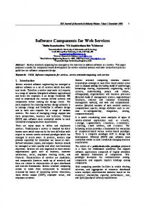
As we have seen, a foundation for modeling software components must also be suitable for expressing compositional styles, scripts, coordination abstractions and glue code. Let us examine each of these in turn to see which requirements they pose. Figure 1 summarizes these requirements, and illustrates how Piccola and the Piccola calculus support them.

A Calculus for Modeling Software Components

3

Glue Piccola • extensible, immutable records • first-class, monadic services • language bridging • introspection • explicit namespaces • services as operators • dynamic scoping on demand • agents & channels

• generic wrappers • component packaging • generic adaptors

Styles • primitive neutral object model • meta-objects • HO plugs & connectors • default arguments • encapsulation • component algebras

Scripts Coordination • coordination abstractions

• sandboxes • composition expressions • context-dependent policies

Fig. 1. How Piccola supports composition

2.1

Compositional Styles

A compositional style allows us to express the structure of a software application in terms of components, connectors and rules governing their composition (cf. “architectural style” [42]). – Neutral object model: There exists a wide variety of different object and component models. Components may also be bigger or smaller than objects. As a consequence, a general foundation for modeling components should make as few assumptions about objects, classes and inheritance as possible, namely, objects provide services, they may be instantiated, and their internal structure is hidden. – Meta-objects: On the other hand, many component models depend on runtime reflection, so it must be possible to express dynamic generation of metaobjects. – Higher-order plugs and connectors: In general, connectors can be seen as higher-order operators over components and other connectors. – Default arguments: Flexibility in plugging together components is achieved if interface dependencies are minimized. Keyword-based rather than positional arguments to services enable both flexibility and extensibility. – Encapsulation: Components are black-box entities that, like objects, provide services, without exposing their structure. At the same time, the components and connectors of a particular style can be encapsulated as a module, or namespace within which components may be scripted.

4

Oscar Nierstrasz and Franz Achermann

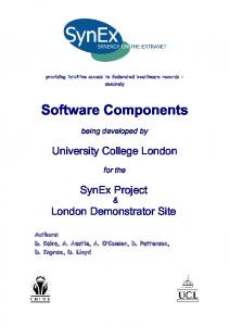
Fig. 2. Evaluating the helloButton script

– Component algebras: Compositional styles are most expressive when compositions of components and connectors again yield components (or connectors). (The composition of two filters is again a filter.) Based on these requirements, we conclude that we need (at least) records (to model objects and components), higher-order functions, reflection, and (at some level) overloading of operators. Services may be monadic, taking records as arguments, rather than polyadic. To invoke a service, we just apply it to a record which bundles together all the required arguments, and possibly some optional ones. These same records can serve as first-class namespaces which encapsulate the plugs and connectors of a given style. For this reason we unify records and namespaces, and call them “forms”, to emphasize their special role. A “form” is essentially a nested record, which binds labels to values. Consider, for example, the following JPiccola script [30]: makeFrame title = "AWT Demo" x = 200 y = 100 hello = "hello world" sayHello: println hello component = Button.new(text=hello) ? ActionPerformed sayHello This script invokes an abstraction makeFrame, passing it a form containing bindings for the labels title, x, and so on. The script makes use of a compositional style in which GUI components (i.e., the Button) can be bound to events (i.e., ActionPerformed) and actions (i.e., sayHello) by means of the ? connector. When we evaluate this code, it generates the button we see in figure 2. When we click on the button, hello world is printed on the Java console. 2.2

Glue

Glue code is needed to package, wrap or adapt code to fit into a compositional style. – Generic wrappers: Wrappers are often needed to introduce specific policies (such as thread-safe synchronization). Generic wrappers are hard to specify

A Calculus for Modeling Software Components

5

for general, polyadic services, but are relatively straightforward if all services are monadic. – Component packaging: Glue code is sometimes needed to package existing code to conform to a particular component model or style. For this purpose, a language bridge is needed to map existing language constructs to the formal component model. – Generic adaptors: Adaptation of interfaces can also be specified generically with the help of reflective or introspective features, which allow components to be inspected before they are adapted. The JPiccola helloButton script only works because Java GUI components are wrapped to fit into our compositional style. In addition to records and higher-order functions over records, we see that some form of language bridging will be needed, perhaps not at the level of the formal model, but certainly for a practical language or system based on the model. 2.3

Scripts

Scripts configure and compose components using the connectors defined for a style. – Sandboxes: For various reasons we may wish to instantiate components only in a controlled environment. We do not necessarily trust third-party components. Sometimes we would like to adapt components only within a local context. For these and other reasons it is convenient to be able to instantiate and compose namespaces which serve as sandboxes for executing scripts. – Composition expressions: Scripts instantiate and connect components. A practical language might conveniently represent connectors as operators. Pipes and filters connections are well-known, but this idea extends well to other domains. – Context-dependent policies: Very often, components must be prepared to employ services of the dynamic context. Transaction services, synchronization or communication primitives may depend on the context. For this reason, pure static scoping may not be enough, and dynamic scoping on demand will be needed for certain kinds of component models. So, we see that explicit, manipulable namespaces become more important. 2.4

Coordination

CBSD is especially relevant in concurrent and distributed contexts. For this reason, a foundation for composition must be able to express coordination of interdependent tasks. – Coordination abstractions: Both connectors and glue code may need to express coordination of concurrent activities. Consider a readers/writers synchronization policy as a generic wrapper.

6

Oscar Nierstrasz and Franz Achermann

We conclude that we not only need higher-order functions over first-class namespaces (with introspection), but also a way of expressing concurrency and communication [40].

3

The Piccola Calculus

As a consequence of the requirements we have identified above, we propose as a foundation a process calculus based on the higher-order asynchronous π calculus [25, 36] in which tuple-based communication is replaced by communication of extensible records, or forms [5]. Furthermore, forms serve as first-class namespaces and support a simple kind of introspection. The design of the Piccola calculus strikes a balance between minimalism and expressiveness. As a calculus it is rather large. In fact, it would be possible to express everything we want with the π calculus alone, but the semantic gap between concepts we wish to model and the terms of the calculus would be rather large. With the Piccola calculus we are aiming for the smallest calculus with which we can conveniently express components, connectors and scripts. 3.1

Syntax

The Piccola calculus is given by agents A, B, C that range over the set of agents A in 1. There are two categories of identifiers: labels and channels. The set of labels L is ranged over by x, y, z. (We use the term “variables” and “labels” interchangeably.) Specific labels are also written in the italic text font. Channels are denoted by a, b, c, d ∈ N . Labels are bound with bindings and λ-abstractions, and channels are bound by ν-restrictions. The operators have the following precedence: application > extension > restriction, abstraction > sandbox > parallel Agent expressions are reduced to static form values or simply forms. Forms are ranged over by F, G, H. Notice that the set of forms is a subset of all agents. Forms are the first-class citizens of the Piccola calculus, i.e., they are the values that get communicated between agents and are used to invoke services. Forms are sets of bindings and services. The set of forms is denoted by F. Certain forms play the role of services. We use S to range over services. User-defined services are closures. Primitive services are inspect, the bind and hide primitives, and the output service. Before considering the formal reduction relation, we first give an informal description of the different agent expressions and how they reduce. – The empty form, , does not reduce further. It denotes a form without any binding. – The current root agent, R, denotes the current lexical scope. – A sandbox A; B evaluates the agent B in the root context given by A. A binds all free labels in B. If B is a label x, we say that A; x is a projection on x in A.

A Calculus for Modeling Software Components

 A; B x7→ L λx.A νc.A c?

empty form sandbox bind inspect abstraction restriction input

| | | | | | |

F, G, H ::=  | x7→F

empty form binding

|S service | F · G extension

A, B, C ::= | | | | | |

S ::= F ; λx.A closure | x7→ bind | c output

R x hide x A·B AB A|B c

7

current root variable hide extension application parallel output

|L inspect | hide x hide

Table 1. Syntax of the Piccola Calculus

– A label, x, denotes the value bound by x in the current root context. – The primitive service bind creates bindings. If A reduces to F , then x7→A reduces to the binding x7→F . – The primitive service hide x removes bindings. So, hide x (x7→ · y 7→) reduces to y 7→. – The inspect service, L, can be used to interate over the bindings and services of an arbitrary form F . The result of LF is a service that takes as its argument a form that binds the labels isEmpty, isService and isLabel to services. One of these three services will then be selected, depending on whether F is , contains some bindings, or is only a service. – The values of two agents are concatenated by extension. In the value of A · B the bindings of B override those for the same label in A. – An abstraction λx.A abstracts x in A. – The application AB denotes the result of applying A to B. Piccola uses a call-by-value reduction order. In order to reduce AB, A must reduce to a service and B to a form. – The expression νc.A restricts the visibility of the channel name c to the agent expression A, as in the π calculus. – A | B spawns off the agent A asynchronously and yields the value of B. Unlike in the π calculus, the parallel composition operator is not commutative, since we do not wish parallel agents to reduce to non-deterministic values. – The agent c? inputs a form from channel c and reduces to that value. The reader familiar with the π-calculus will notice a difference with the input prefix. Since we have explicit substitution in our calculus it is simpler to specify the input by c? and use the context to bind the received value instead of defining a prefix syntax c(X).A as in the π-calculus. – The channel c is a primitive output service. If A reduces to F , then cA reduces to the message cF . The value of a message is the empty form . (The value F is only obtained by a corresponding input c? in another agent.)

8

Oscar Nierstrasz and Franz Achermann

fc() fc(x) fc(x7→) fc(A; B) fc(λx.A) fc(νc.A) fc(c?)

= = = = = = =

∅ ∅ ∅ fc(A) ∪ fc(B) fc(A) fc(A)\{c} {c}

fc(R) fc(L) fc(hide x ) fc(A · B) fc(AB) fc(A | B) fc(c)

= = = = = = =

∅ ∅ ∅ fc(A) ∪ fc(B) fc(A) ∪ fc(B) fc(A) ∪ fc(B) {c}

Table 2. Free Channels

3.2

Free Channels and Closed Agents

As in the π-calculus, forms may contain free channel names. An agent may create a new channel, and communicate this new name to another agent in a separate lexical scope. The free channels fc(A) of an agent A are defined inductively in table 2. αconversion (of channels) is defined in the usual way. We identify agent expressions up to α-conversion. We omit a definition of free variables. Since Piccola is a calculus with explicit environments, we cannot easily define α-conversion on variables. Such a definition would have to include the special nature of R. Instead, we define a closed agent where all variables, root expressions, and abstractions occur beneath a sandbox: Definition 1. The following agents A are closed: – , x7→, hide x , L, c and c? are closed. – If A and B are closed then also A · B, AB, A | B and νc.A are closed. – If A is closed, then also A; B is also closed for any agent B. Observe that any form F is closed by the above definition. An agent is open if it is not closed. Open agents are R, variables x, abstractions λx.A and compositions thereof. Any agent can be closed by putting it into a sandbox with a closed context. Sandbox agents are closed if the root context is closed. In lemma 1 we show that the property of being closed is preserved by reduction. 3.3

Congruence and Pre-forms

As in the π calculus, we introduce structural congruence over agent expressions to simplify the reduction relation. The congruence allows us to rewrite agent expressions to bring communicating agents into juxtapositions, as in the Chemical Abstract Machine of Berry and Boudol [8]. The congruence rules constitute three groups (see table 3). The first group (from ext empty right to single service) deals with congruence over forms. It specifies that extension is idempotent and associative on forms.

A Calculus for Modeling Software Components

9

≡ is the smallest congruence satisfying the following axioms:

x 6= y

implies

x 6= y

implies

c∈ / fc(A) c∈ / fc(A) c∈ / fc(A) c∈ / fc(A) c∈ / fc(A) c∈ / fc(A) c∈ / fc(A) c∈ / fc(A)

implies implies implies implies implies implies implies implies

F · ·F (F · G) · H S · (x7→F ) x7→F · y 7→G x7→F · x7→G S · S0 F;A · B F ; AB A; (B; C) F;G F;R hide x (F · x7→G) hide y (F · x7→G) hide x  hide x S (F · S)G (A | B) | C (A | B) | C (A | B) · C F · (A | B) (A | B)C F (A | B) (A | B); C F ; (A | B) F |A cF νcd.A A | νc.B (νc.B) | A (νc.B) · A A · νc.B A; νc.B (νc.B); A (νc.B)A A(νc.B)

≡ ≡ ≡ ≡ ≡ ≡ ≡ ≡ ≡ ≡ ≡ ≡ ≡ ≡ ≡ ≡ ≡ ≡ ≡ ≡ ≡ ≡ ≡ ≡ ≡ ≡ ≡ ≡ ≡ ≡ ≡ ≡ ≡ ≡ ≡ ≡

F (ext empty right) F (ext empty left) F · (G · H) (ext assoc) (x7→F ) · S (ext service commute) y 7→G · x7→F (ext bind commute) x7→G (single binding) S0 (single service) (F ; A) · (F ; B) (sandbox ext) (F ; A)(F ; B) (sandbox app) (A; B); C (sandbox assoc) G (sandbox value) F (sandbox root) hide x F (hide select) hide y F · x7→G (hide over)  (hide empty) S (hide service) SG (use service) A | (B | C) (par assoc) (B | A) | C (par left commute) A | B·C (par ext left) A | F ·B (par ext right) A | BC (par app left) A | FB (par app right) A | B; C (par sandbox left) F;A | F;B (par sandbox right) A (discard zombie) cF |  (emit) νdc.A (commute channels) νc.(A | B) (scope par left) νc.(B | A) (scope par right) νc.(B · A) (scope ext left) νc.(A · B) (scope ext right) νc.(A; B) (scope sandbox left) νc.(B; A) (scope sandbox right) νc.BA (scope app left) νc.AB (scope app right)

Table 3. Congruences

10

Oscar Nierstrasz and Franz Achermann

The rules single service and single binding specify that extension overwrites services and bindings with the same label. We define labels(F ) as follows: Definition 2. For each form F , the set of labels(F ) ⊂ L is given by: labels() = ∅ labels(x7→G) = {x}

labels(S) = ∅ labels(F · G) = labels(F ) ∪ labels(G)

Using the form congruences, we can rewrite any form F into one of the following three cases: F ≡ F ≡S F ≡ F 0 · x7→G

where x 6∈ labels(F 0 )

This is proved by structural induction over forms [2]. This formalizes our idea that forms are extensible records unified with services. A form has at most one binding for a given label. The second group (from sandbox ext to use service) defines preforms. These are agent expressions that are congruent to a form. For instance, the agent hide x  is equivalent to the empty form . The set of all preforms is defined by: F ≡ = {A|∃F ∈ F with F ≡ A} Clearly, all forms are preforms. The last group (from par assoc to scope app right) defines the semantics of parallel composition and communication for agents. Note how these rules always preserve the position of the rightmost agent in a parallel composition, since this agent, when reduced to a form, will represent the value of the composition. In particular, the rule discard zombie garbage-collects form values appearing to the left of this position. The rule emit, on the other hand, spawns an empty form as the value, thus enabling the message to move around freely. For instance in x7→c() ≡ x7→(c() | ) ≡ c() | x7→

by emit by par ext right

the message c() escapes the binding x7→. 3.4

Reduction

We define the reduction relation → on agent expressions to reduce applications, communications and projections (see table 4). ⇒ is the reflexive and transitive closure of →. Especially noteworthy is the rule reduce beta. This rule does not substitute G for x in the agent A as in the classical λ-calculus. Instead, it extends the

A Calculus for Modeling Software Components

11

(F ; λx.A) G → F · x7→G; A

(reduce beta)

cF | c? → F

(reduce comm)

F · x7→G; x → G

(reduce project)

L → ; λx.(x; isEmpty)

(reduce inspect empty)

LS → ; λx.(x; isService)

(reduce inspect service)

L(F · x7→G) → ; λx.(x; isLabel )label x

(reduce inspect label)

0

0

A≡A

A →B

0

0

B ≡B

(reduce struct)

A→B A→B E[A] → E[B]

(reduce propagate)

where label x = project 7→(; λx.(x; x)) · hide 7→hide x · bind 7→(x7→) and E is an evaluation context defined by the grammar: E ::= [ ] E · A F · E E; A F ; E EA F E A|E E|A νc.E Table 4. Reduction rules

environment in which A is evaluated. This is essentially the beta-reduction rule found in calculi for explicit substitution [1, 32]: (F ; λx.A)G → F · x7→G; A The application of the closure F ; λx.A to the argument G reduces to a sandbox expression in which the agent A is evaluated in the environment F · x7→G. Free occurrences of x in A will therefore be bound to G. The property of being closed is respected by reduction: Lemma 1. If A is a closed agent and A → B or A ≡ B then B is closed as well. Proof. Easily checked by induction over the formal proof for A → B.

3.5

Encoding Booleans

The following toy example actually illustrates many of the principles at stake when we model components with the Piccola calculus. We can encode booleans by services that either project on the labels true or false depending on which boolean value they are supposed to model (cf. [13]). (This same idea is used by the primitive service L to reflect over the bindings and services of a form.)

12

Oscar Nierstrasz and Franz Achermann

def

True = ; λx.(x; true)

(1)

def

False = ; λx.(x; false)

(2)

Consider now: True(true 7→1 · false 7→2) = (; λx.(x; true))(true 7→1 · false 7→2) →  · x7→(true 7→1 · false 7→2); (x; true) by reduce beta ≡ ( · x7→(true 7→1 · false 7→2); x); true by sandbox assoc → (true 7→1 · false 7→2); true by reduce project ≡ (false 7→2 · true 7→1); true by ext bind commute →1 by reduce project Note how the bindings are swapped to project on true in the last step. A similar reduction would show False(true 7→1 · false 7→2) ⇒ 2. One of the key points of forms is that a client can provide additional bindings which are ignored when they are not used (cf. [13]). This same principle is applied to good effect in various scripting languages, such as Python [22]. For instance we can use True and provide an additional binding notused 7→F for arbitrary form F :

True(true 7→1 · false 7→2 · notused 7→F ) ⇒ (true 7→1 · false 7→2 · notused 7→F ); true ≡ (false 7→2 · true 7→1 · notused 7→F ); true ≡ (false 7→2 · notused 7→F · true 7→1); true →1

by ext bind commute by ext bind commute by reduce project

Extending forms can also be used to overwrite existing bindings. For instance instead of binding the variable notused a client may override true: True(true 7→1 · false 7→2 · true 7→3) ⇒ 3 A conditional expression is encoded as a curried service that takes a boolean and a case form. When invoked, it selects and evaluates the appropriate service in the case form: def

if = ; λuv.u(true 7→(v; then) · false 7→(v; else)) Now consider: if True (then 7→(F ; λx.A) · else 7→(G; λx.B)) ⇒ F · x7→; A

A Calculus for Modeling Software Components

13

The expression if True has triggered the evaluation of agent A in the environment F · x7→. The contract supported by if requires that the cases provided bind the labels then and else. We can relax this contract and provide default services if those bindings are not provided by the client. To do so, we replace in the definition of if the sandbox expression v; else with a default service. This service gets triggered when the case form does not contain an else binding: def

ifd = ; λuv.b(true 7→(v; then) · false 7→(else 7→(λx.) · v; else)) Now ifd False(then 7→(F ; λx.A)) ⇒ . 3.6

Equivalence for Agents

Two agents are equivalent if they exhibit the same behaviour, i.e., they enjoy the same reductions. We adopt Milner and Sangiorgi’s notion of barbed bisimulation [26]. The idea is that an agent A is barbed similar to B if A can exhibit any reduction that B does and if B is a barb, then A is a barb, too. If A and B are similar to each other they are bisimilar. The advantage of this bisimulation is that it can be readily be given for any calculus that contains barbs or values. For the asynchronous π-calculus, barbs are usually defined as having the capability of doing an output on a channel. A Piccola agent reduces to a barb, i.e., it returns a form. During evaluation the agent may spawn off new subthreads which could be blocked or still be running. We consequently define barbs as follows: Definition 3. A barb V is an agent expression A that is congruent to an agent generated by the following grammar: V ::= F A|V νc.V We write A ↓ for the fact that A is a barb, and A ⇓ when a barb V exists such that A ⇒ V . The following lemma relates forms, barbs and agents: Lemma 2. The following inclusion holds and is strict: F ⊂ F ≡ ⊂ {A|A ↓} ⊂ A Proof. The inclusions hold by definition. To see that the inclusion are strict, consider the empty form , the agent hide x , the barb 0 | hide x  and the agent 0 (where 0 = νc.c? is the deadlocked null agent). The following lemma gives a syntactical characterization of barbs.

14

Oscar Nierstrasz and Franz Achermann

Lemma 3. For any form F , agent A, and label x, the following terms are barbs, given V1 and V2 are barbs. V1 · V2 V1 ; V 2 x7→V1

νc.V1 A | V1

Proof. By definition we have V ≡ ν˜ c.A | F . The claim follows by induction over F. We now define barbed bisimulation and the induced congruence: Definition 4. A relation R is a (weak) barbed bisimulation, if A R B, i.e., (A, B) ∈ R implies: – – – –

If If If If

A → A0 then there exists an agent B 0 with B ⇒ B 0 and A0 R B 0 . B → B 0 then there exists an agent A0 with A ⇒ A0 and A0 R B 0 . A ↓ then B ⇓. B ↓ then A ⇓.

˙ B, if there is some (weak) Two agents are (weakly) barbed bisimilar, written A ≈ barbed bisimulation R with A R B. Two agents are (weakly) barbed congruent, ˙ C[B]. written A ≈ B, if for all contexts C we have C[A] ≈ We define behavioural equality using the notion of barbed congruence. As usual we can define strong and weak versions of barbed bisimulation. The strong versions are obtained in the standard way by replacing ⇒ with → and ⇓ with ↓ in Definition 4. We only concentrate on the weak case since it abstracts internal computation. 3.7

Erroneous Reductions

Not all agents reduce to forms. Some agents enjoy an infinite reduction [2]. Other agents are stuck. An agent is stuck if it is not a barb and can reduce no further. Definition 5. An agent A is stuck, written A ↑, if A is not a barb and there is no agent B such that A → B. Clearly it holds that 0 ↑ and R ↑. The property of being stuck is not compositional. For instance c? ↑ but obviously, c() | c? can reduce to . We can put R into a context so that it becomes a barb, for instance F ; R ≡ F . Note that if an agent is stuck it is not a preform: F ≡ ∩ {A|A ↑} = ∅ by definition. Although 0 is arguably stuck by intention, in general a stuck agent can be interpreted as an error. The two typical cases which may lead to errors are (i) projection on an unbound label, e.g., ; x, and (ii) application of a non-service, e.g., .

A Calculus for Modeling Software Components

3.8

15

π-Calculus Encoding

One may well ask what exactly the Piccola calculus adds over and above the asynchronous π calculus. In Achermann’s thesis it is shown that the Piccola calculus can be faithfully embedded into the localized π-calculus Lπ of Merro and Sangiorgi [23, 36]. The mapping [[]]a encodes Piccola calculus agents as π-calculus processes. The process [[A]]a evaluates A in the environment given by the empty form, and sends the resulting value along the channel a. A form (value) is encoded as a 4-tuple of channels representing projection, invocation, hiding and selection. The main result is that the encoding is sound and preserves reductions. We do not require a fully abstract encoding since that would mean that equivalent Piccola agents translated into the π-calculus could not be distinguished by any π-processes. Our milder requirement means that we consider only π-processes which are translations of Piccola agents themselves and state that they cannot distinguish similar agents: Proposition 1 (Soundness). For closed agents A, B and channel a the congruence [[A]]a ≈ [[B]]a implies A ≈ B. Although it is comforting to learn that the π-calculus can serve as a foundation for modeling components, it is also clear from the complexity of the encoding that it is very distant from the kinds of abstractions we need to conveniently model software composition. For this reason we find that a richer calculus is more convenient to express components and connectors.

4

From the Piccola Calculus to Piccola

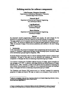
Piccola is a small composition language that supports the requirements summarized in figure 1, and whose denotational semantics is defined in terms of the Piccola calculus [2]. Piccola is designed in layered fashion. At the lowest level we have an abstract machine that implements the Piccola calculus. At the next level, we have the Piccola language, which is implemented by translation to the abstract machine, following the specification of the denotational semantics. Applications: Composition styles: Standard libraries:

Piccola language:

Piccola calculus:

Piccola Layers Components + Scripts Streams, GUI composition, ... Coordination abstractions, control structures, basic object model ... Host components, user-defined operators, dynamic namespaces Forms, agents and channels

16

Oscar Nierstrasz and Franz Achermann

Piccola provides a more convenient, Python-like syntax for programming than does the calculus, including overloaded operators to support algebraic component composition. It also provides a bridge to the host language (currently Java or Squeak). Piccola provides no basic data types other than forms and channels. Booleans, integers, floating point numbers and strings, for example, must be provided by the host language through the language bridge. Curiously, the syntax of the Piccola calculus is actually larger than that of Piccola itself. This is because we need to represent all semantic entities, including agents and channels, as syntactic constructs in the calculus. In the Piccola language, however, these are represented only by standard library services, such as run and newChannel. The next layer provides a set of standard libraries to simplify the task of programming with Piccola. Not only does the Piccola language provide no built-in data types, it does not even offer any control structures of its own. These, however, are provided as standard services implemented in Piccola. Exceptions and try-catch clauses are implemented using agents, channels, and dynamic namespaces [5]. The first three layers constitute the standard Piccola distribution. The fourth layer is provided by the component framework designer. At this level, a domain expert encodes a compositional styles as a library of components, connectors, adaptors, coordination abstractions, and so on. Finally, at the top level, an application programmer may script together components using the abstractions provided by the lower layers [3, 29]. 4.1

Reasoning About Styles

We have also explored how to reason about Piccola programs at the language level [2]. We have studied two extended examples. First, we considered synchronization wrappers that express the synchronization constraints assumed by a component. We can use synchronization wrappers to make components safe in a multithreaded environment. The wrappers separate the functionality of the component from their synchronization aspects. If the constraints assumed by the component hold in a particular composition the wrapper is not needed. In particular the wrapper is not necessary when the component is already wrapped. This property is formally expressed by requiring that the wrappers be idempotent. The second study compares push- and pull-flow filters. We demonstrate how to adapt pull-filters so that they work in a push-style. We have constructed a generic adapter for this task in two iterations. The first version contains a racecondition that may lead to data being lost. The formal model of Piccola is used to analyze the traces of an adapted filter and helps to detect the error. To fix the problem we specify the dynamics of a push-style filter, namely that push and close calls be mutually exclusive, that no further push calls may be attempted after a close, and that no “air-bubble” elements (filter slots holding an empty form) may be pushed downstream.

A Calculus for Modeling Software Components

17

Having clarified the interaction protocol as a wrapper, we present an improved version of the generic adapter. We show that the adapter ensures these invariants. 4.2

Partial Evaluation

Another interesting application of the calculus was to enable the efficient implementation of the language bridge. Since Piccola is a pure composition language, evaluating scripts requires intensive upping and downing [24] between the “down” level of the host language and the “up” level of Piccola. If the language bridge were implemented na¨ıvely, it would be hopelessly inefficient. Instead, Piccola achieves acceptable performance by adopting a partial evaluation scheme [2, 38, 39]. Since the language has a denotational semantics, we can implement it efficiently while proving that we preserve the intended semantics. The partial evaluation algorithm uses the fact that forms are immutable. We replace references to forms by the forms referred to. We can then specialize projections and replace applications of referentially transparent services by their results. However, most services in Piccola are not referentially transparent and cannot be inlined since that would change the order in which side-effects are executed. We need to separate the referentially transparent part from the non-transparent part in order to replace an application with its result and to ensure that the order in which the side-effects are evaluated is preserved. At the heart of the proof is that we can separate form expressions into sideeffects and referentially transparent forms [2].

5

Related Work

The Piccola calculus extends the asynchronous π-calculus with higher-order abstractions and first-class environments. π-calculus. The π-calculus [25] is a calculus of communicating systems in which one can naturally express processes with a changing structure. Its theory has been thoroughly studied and many results relate other formalisms or implementations to it. The affinity between objects and processes, for example, has been treated by various authors in the context of the π-calculus [18, 44]. The Pict experiment has shown that the π-calculus is a suitable basis for programming many high-level construct by encodings [33]. For programming and implementation purposes, synchronous communication seems uncommon and can generally be encoded by using explicit acknowledgments (cf. [18]). Moreover, asynchronous communication has a closer correspondence to distributed computing [45]. Furthermore, in the π-calculus the asynchronous variant has the pleasant property that equivalences are simpler than for the synchronous case [14]. Input-guarded choice can be encoded and is fully abstract [27]. For these reasons we adopt asynchronous channels in Piccola.

18

Oscar Nierstrasz and Franz Achermann

Higher-order abstractions. Programming directly in the π-calculus is often considered like programming a concurrent assembler. When comparing programs written in the π-calculus with the lambda-calculus it seems like lambda abstractions scale up, whereas sending and receiving messages does not scale well. There are two possible solutions proposed to this problem: We can change the metaphor of communication or we can introduce abstractions as first-class values. The first approach is advocated by the Join-calculus [15]. Communication does not happen between a sender and a receiver, instead a join pattern triggers a process on consumption of several pending messages. The Blue calculus of Boudol [9] changes the receive primitive into a definition which is defined for a scope. By that change, the Blue calculus is more closely related to functions and provides a better notion for higher-order abstraction. Boudol calls it a continuation-passing calculus. The other approach is adopted by Sangiorgi in the HOπ-calculus. Instead of communicating channels or tuples of channels, processes can be communicated as well. Surprisingly, the higher-order case has the same expressive power as the first-order version [35, 36]. In Piccola we take the second approach and reuse existing encodings of functions into the π-calculus as in Pict. The motivation for this comes from the fact that the HOπ-calculus itself can be encoded in the first-order case. Asymmetric parallel composition. The semantics of asynchronous parallel composition is used in the concurrent object calculus of Gordon and Hankin [17] or the (asymmetric) Blue calculus studied by Dal-Zilio [12]. In the higher-order π-calculus the evaluation order is orthogonal to the communication semantics [36]. In Piccola, evaluation strategy interferes with communication, therefore we have to fix one for meaningful terms. For Piccola, we define strict evaluation which seems appropriate and more common for concurrent computing. Record calculus. When modeling components and interfaces, a record-based approach is the obvious choice. We use forms [20, 21] as an explicit notion for extensible records. Record calculi are studied in more detail for example in [11, 34]. In the λ-calculus with names of Dami [13] arguments to functions are named. The resulting system supports records as arguments instead of tuples as in the classical calculus. The λN -calculus was one of the main inspiration for our work on forms without introspection. An issue omitted in our approach is record typing. It is not clear how far record types with subtyping and the runtime acquisition can be combined. An overview of record typing and the problems involved can be found for example in [11]. Explicit environments. An explicit environment generalizes the concept of explicit substitution [1] by using a record like structure for the environment. In the environment calculus of Nishizaki, there is an operation to get the current environment as a record and an operator to evaluate an expression using a record as environment [32, 37]. Projection of a label x in a record R then corresponds

A Calculus for Modeling Software Components

19

to evaluating the script x in an environment denoted by R. The reader may note that explicit environments subsume records. This is the reason why we call them forms in Piccola instead of just records. Handling the environment as a first-class entity allows us to define concepts like modules, interfaces and implementation for programming in the large within the framework. To our knowledge, the language Pebble of Burstall and Lampson was the first to formally show how to build modules, interfaces and implementation, abstract data types and generics on a typed lambda calculus with bindings, declarations and types as first-class values [10]. Other approaches A very different model is offered by ρω (AKA Reo) [7], a calculus of component connectors. Reo is algebraic in flavour, and provides various connectors that coordinate and compose streams of data. Primitives connectors can be composed using the Reo operators to build hiigher-level connectors. In contrast to process calculi, Reo is well-suited to compositional reasoning, since connectors can be composed to yield new connectors, and properties of connectors can be shown to compose. Data communicated along streams are uninterpreted in Reo, so it would be natural to explore the application of Reo to streams of forms.

6

Concluding Remarks

We have presented the Piccola calculus, a high-level calculus for modeling software components that extends the asynchronous π-calculus with explicit namespaces, or forms. The calculus serves as the semantic target for Piccola, a language for composing software components that conform to a particular compositional style. JPiccola, the Java implementation of Piccola, is realized by translation to an abstract machine that implements the Piccola calculus. The Piccola calculus is not only helpful for modeling components and connectors, but it also helps to reason about the Piccola language implementation and about compositional styles. Efficient language bridging between Piccola and the host language (Java or Squeak) is achieved by means of partial evaluation of language wrappers. The partial evaluation algorithm can be proved correct with the help of the Piccola calculus. Different compositional styles make different assumptions about software components. Mixing incompatible components can lead to compositional mismatches. We have outlined how the Piccola calculus can help to bridge mismatches by supporting reasoning about wrappers that adapt component contracts from one style to another. One shortcoming of our work so far is the lack of a type system. We have been experimenting with a system of contractual types [28] that expresses both the provided as well as the required services of a software component. Contractual types are formalized in the context of the form calculus, which can be seen as the Piccola calculus minus agents and channels. Contractual types have been integrated into the most recent distribution of JPiccola [19].

20

Oscar Nierstrasz and Franz Achermann

Acknowledgments We gratefully acknowledge the financial support of the Swiss National Science Foundation for projects No. 20-61655.00, “Meta-models and Tools for Evolution Towards Component Systems”, and 2000-067855.02, “Tools and Techniques for Decomposing and Composing Software”.

References 1. Mart´ın Abadi, Luca Cardelli, Pierre-Louis Curien, and Jean-Jacques L´evy. Explicit substitutions. Journal of Functional Programming, 1(4):375–416, October 1991. 2. Franz Achermann. Forms, Agents and Channels – Defining Composition Abstraction with Style. PhD thesis, University of Berne, January 2002. 3. Franz Achermann, Stefan Kneubuehl, and Oscar Nierstrasz. Scripting coordination styles. In Ant´ onio Porto and Gruia-Catalin Roman, editors, Coordination ’2000, volume 1906 of LNCS, pages 19–35, Limassol, Cyprus, September 2000. SpringerVerlag. 4. Franz Achermann, Markus Lumpe, Jean-Guy Schneider, and Oscar Nierstrasz. Piccola – a small composition language. In Howard Bowman and John Derrick, editors, Formal Methods for Distributed Processing – A Survey of Object-Oriented Approaches, pages 403–426. Cambridge University Press, 2001. 5. Franz Achermann and Oscar Nierstrasz. Explicit Namespaces. In J¨ urg Gutknecht and Wolfgang Weck, editors, Modular Programming Languages, volume 1897 of LNCS, pages 77–89, Z¨ urich, Switzerland, September 2000. Springer-Verlag. 6. Franz Achermann and Oscar Nierstrasz. Applications = Components + Scripts – A Tour of Piccola. In Mehmet Aksit, editor, Software Architectures and Component Technology, pages 261–292. Kluwer, 2001. 7. Farhad Arbab and Farhad Mavaddat. Coordination through channel composition. In F. Arbab and C. Talcott, editors, Coordination Languages and Models: Proc. Coordination 2002, volume 2315 of Lecture Notes in Computer Science, pages 21– 38. Springer-Verlag, April 2002. 8. G´erard Berry and G´erard Boudol. The chemical abstract machine. Theoretical Computer Science, 96:217–248, 1992. 9. G´erard Boudol. The pi-calculus in direct style. In Conference Record of POPL ’97, pages 228–241, 1997. 10. Rod Burstall and Butler Lampson. A kernel language for abstract data types and modules. Information and Computation, 76(2/3), 1984. Also appeared in Proceedings of the International Symposium on Semantics of Data Types, Springer, LNCS (1984), and as SRC Research Report 1. 11. Luca Cardelli and John C. Mitchell. Operations on records. In Carl A. Gunter and John C. Mitchell, editors, Theoretical Aspects of Object-Oriented Programming. Types, Semantics and Language Design, pages 295–350. MIT Press, 1993. 12. Silvano Dal-Zilio. Le calcul bleu: types et objects. Ph.D. thesis, Universit´e de Nice – Sophia Antipolis, July 1999. In french. 13. Laurent Dami. Software Composition: Towards an Integration of Functional and Object-Oriented Approaches. Ph.D. thesis, University of Geneva, 1994. 14. C´edric Fournet and Georges Gonthier. A hierarchy of equivalences for asynchronous calculi. In Proceedings of ICALP ’98, pages 844–855, 1998.

A Calculus for Modeling Software Components

21

15. C´edric Fournet, Georges Gonthier, Jean-Jacques L´evy, Luc Maranget, and Didier R´emy. A calculus of mobile agents. In Proceedings of the 7th International Conference on Concurrency Theory (CONCUR ’96), volume 1119 of LNCS, pages 406–421. Springer-Verlag, August 1996. 16. David Garlan, Robert Allen, and John Ockerbloom. Architectural mismatch: Why reuse is so hard. IEEE Software, 12(6):17–26, November 1995. 17. Andrew D. Gordon and Paul D. Hankin. A concurrent object calculus: Reduction and typing. In Proceedings HLCL ’98. Elsevier ENTCS, 1998. 18. Kohei Honda and Mario Tokoro. An object calculus for asynchronous communication. In Pierre America, editor, Proceedings ECOOP ’91, volume 512 of LNCS, pages 133–147, Geneva, Switzerland, July 15–19 1991. Springer-Verlag. 19. Stefan Kneubuehl. Typeful compositional styles. Diploma thesis, University of Bern, April 2003. 20. Markus Lumpe. A Pi-Calculus Based Approach to Software Composition. Ph.D. thesis, University of Bern, Institute of Computer Science and Applied Mathematics, January 1999. 21. Markus Lumpe, Franz Achermann, and Oscar Nierstrasz. A Formal Language for Composition. In Gary Leavens and Murali Sitaraman, editors, Foundations of Component Based Systems, pages 69–90. Cambridge University Press, 2000. 22. Mark Lutz. Programming Python. O’Reilly & Associates, Inc., 1996. 23. Massimo Merro and Davide Sangiorgi. On asynchrony in name-passing calculi. In Kim G. Larsen, Sven Skyum, and Glynn Winskel, editors, 25th Colloquium on Automata, Languages and Programming (ICALP) (Aalborg, Denmark), volume 1443 of LNCS, pages 856–867. Springer-Verlag, July 1998. 24. Wolfgang De Meuter. Agora: The story of the simplest MOP in the world — or — the scheme of object–orientation. In J. Noble, I. Moore, and A. Taivalsaari, editors, Prototype-based Programming. Springer-Verlag, 1998. 25. Robin Milner, Joachim Parrow, and David Walker. A calculus of mobile processes, part I/II. Information and Computation, 100:1–77, 1992. 26. Robin Milner and Davide Sangiorgi. Barbed bisimulation. In Proceedings ICALP ’92, volume 623 of LNCS, pages 685–695, Vienna, July 1992. Springer-Verlag. 27. Uwe Nestmann and Benjamin C. Pierce. Decoding choice encodings. In Ugo Montanari and Vladimiro Sassone, editors, CONCUR ’96: Concurrency Theory, 7th International Conference, volume 1119 of LNCS, pages 179–194, Pisa, Italy, August 1996. Springer-Verlag. 28. Oscar Nierstrasz. Contractual types. Technical Report IAM-03-004, Institut f¨ ur Informatik, Universit¨ at Bern, Switzerland, 2003. 29. Oscar Nierstrasz and Franz Achermann. Supporting Compositional Styles for Software Evolution. In Proceedings International Symposium on Principles of Software Evolution (ISPSE 2000), pages 11–19, Kanazawa, Japan, Nov 1-2 2000. IEEE. 30. Oscar Nierstrasz, Franz Achermann, and Stefan Kneubuehl. A guide to jpiccola. Technical Report IAM-03-003, Institut f¨ ur Informatik, Universit¨ at Bern, Switzerland, June 2003. 31. Oscar Nierstrasz and Laurent Dami. Component-oriented software technology. In Oscar Nierstrasz and Dennis Tsichritzis, editors, Object-Oriented Software Composition, pages 3–28. Prentice-Hall, 1995. 32. Shin-ya Nishizaki. Programmable environment calculus as theory of dynamic software evolution. In Proceedings ISPSE 2000. IEEE Computer Society Press, 2000. 33. Benjamin C. Pierce and David N. Turner. Pict: A programming language based on the pi-calculus. In G. Plotkin, C. Stirling, and M. Tofte, editors, Proof, Language and Interaction: Essays in Honour of Robin Milner. MIT Press, May 2000.

22

Oscar Nierstrasz and Franz Achermann

34. Didier R´emy. Typing Record Concatenation for Free, chapter 10, pages 351–372. MIT Press, April 1994. 35. Davide Sangiorgi. Expressing Mobility in Process Algebras: First-Order and HigherOrder Paradigms. Ph.D. thesis, Computer Science Dept., University of Edinburgh, May 1993. 36. Davide Sangiorgi. Asynchronous process calculi: the first-order and higher-order paradigms (tutorial). Theoretical Computer Science, 253, 2001. 37. Masahiko Sato, Takafumi Sakurai, and Rod M. Burstall. Explicit environments. In Jean-Yves Girard, editor, Typed Lambda Calculi and Applications, volume 1581 of LNCS, pages 340–354, L’Aquila, Italy, April 1999. Springer-Verlag. 38. Nathanael Sch¨ arli. Supporting pure composition by inter-language bridging on the meta-level. Diploma thesis, University of Bern, September 2001. 39. Nathanael Sch¨ arli and Franz Achermann. Partial evaluation of inter-language wrappers. In Workshop on Composition Languages, WCL ’01, September 2001. 40. Jean-Guy Schneider. Components, Scripts, and Glue: A conceptual framework for software composition. Ph.D. thesis, University of Bern, Institute of Computer Science and Applied Mathematics, October 1999. 41. Jean-Guy Schneider and Oscar Nierstrasz. Components, scripts and glue. In Leonor Barroca, Jon Hall, and Patrick Hall, editors, Software Architectures – Advances and Applications, pages 13–25. Springer-Verlag, 1999. 42. Mary Shaw and David Garlan. Software Architecture: Perspectives on an Emerging Discipline. Prentice-Hall, 1996. 43. Clemens A. Szyperski. Component Software. Addison Wesley, 1998. 44. David Walker. Objects in the π-calculus. Information and Computation, 116(2):253–271, February 1995. 45. Pawel T. Wojciechowski. Nomadic Pict: Language and Infrastructure Design for Mobile Computation. PhD thesis, Wolfson College, University of Cambridge, March 2000.