of stages by making the intermediate latches transparent and dis- .... DPS-enabled pipeline resembles the Alpha 21264 seven-stage pipeline. Thus, the ...
A Case for Dynamic Pipeline Scaling Jinson Koppanalil, Prakash Ramrakhyani, Sameer Desai, Anu Vaidyanathan, Eric Rotenberg Department of Electrical and Computer Engineering North Carolina State University Raleigh, NC 27695-7914 (919) 513-2822
{jjkoppan, psramrak, shdesai, avaidya, ericro}@ece.ncsu.edu
ABSTRACT
General Terms
Energy consumption can be reduced by scaling down frequency when peak performance is not needed. A lower frequency permits slower circuits, and hence a lower supply voltage. Energy reduction comes from voltage reduction, a technique called Dynamic Voltage Scaling (DVS).
Design, Performance.
This paper makes the case that the useful frequency range of DVS is limited because there is a lower bound on voltage. Lowering frequency permits voltage reduction until the lowest voltage is reached. Beyond that point, lowering frequency further does not save energy because voltage is constant. However, there is still opportunity for energy reduction outside the influence of DVS. If frequency is lowered enough, pairs of pipeline stages can be merged to form a shallower pipeline. The shallow pipeline has better instructions-per-cycle (IPC) than the deep pipeline. Since energy also depends on IPC, energy is reduced for a given frequency. Accordingly, we propose Dynamic Pipeline Scaling (DPS). A DPS-enabled deep pipeline can merge adjacent pairs of stages by making the intermediate latches transparent and disabling corresponding feedback paths. Thus, a DPS-enabled pipeline has a deep mode for higher frequencies within the influence of DVS, and a shallow mode for lower frequencies. Shallow mode extends the frequency range for which energy reduction is possible. For frequencies outside the influence of DVS, a DPS-enabled deep pipeline consumes from 23% to 40% less energy than a rigid deep pipeline.
Categories and Subject Descriptors C.1.3 [Processor Architectures]: Other Architecture Styles — pipeline processors, adaptable architectures; C.3 [Special-Purpose and Application-Based Systems]: real-time and embedded systems; C.5.3 [Computer System Implementation]: Microcomputers — microprocessors, personal computers, portable devices, workstations.
Keywords Variable-depth pipeline, shallow and deep pipelines, configurable pipeline, power and energy management, dynamic voltage scaling, clock gating, fetch gating.
1. INTRODUCTION Energy consumption can be reduced by adapting processor frequency to changing performance requirements. Lowering frequency permits circuits to run slower, and a way to slow down circuits is to reduce the supply voltage. This is referred to as dynamic voltage scaling (DVS) [16,17,19,22,23,26,27]. While frequency management is the enabler, DVS is the actual source of energy savings because energy depends on the square of voltage. However, at some point, a lower voltage bound is reached and lowering frequency further does not produce additional energy savings. This is shown in Figure 1 for the line labeled “deep pipeline”. Typically, the peak frequency is accommodated by a deep pipeline and a peak voltage setting, Vhigh. Lowering frequency permits reducing the voltage — until the lower voltage bound, Vlow, is reached. Once Vlow is reached, lowering frequency further does not produce energy savings (although power is reduced). So, region A in Figure 1 is the useful frequency range for DVS. For example, the Transmeta TM5800 supports frequencies from 367 MHz to 800 MHz corresponding to voltages of 0.9 V to 1.3 V [12]. Underlying reasons for the limited useful frequency range for DVS are explored in Section 3.
voltage Vhigh
shallow pipeline
deep pipeline
Vlow
Permission to make digital or hard copies of all or part of this work for personal or classroom use is granted without fee provided that copies are not made or distributed for profit or commercial advantage and that copies bear this notice and the full citation on the first page. To copy otherwise, or republish, to post on servers or to redistribute to lists, requires prior specific permission and/or a fee. CASES 2002, October 8-11, 2002, Grenoble, France.
Copyright 2002 ACM 1-58113-575-0/02/0010…$5.00.
frequency region C
region B
region A
Figure 1. Voltage-frequency characteristic.
Fortunately, lowering frequency below the useful frequency range of DVS still holds potential for energy savings. If frequency is lowered enough, pipeline stages can be merged to form a shallower pipeline (fewer pipeline stages). The advantage of doing this is that the shallower pipeline has better instructions-per-cycle (IPC) than the deep pipeline. And energy depends not only on voltage, but also IPC, as derived below. 2
# instr. f ⋅ IPC
V IPC
(EQ 1)
Accordingly, we propose dynamic pipeline scaling (DPS), a coarse-grain pipeline reconfiguration technique for extending the frequency range over which energy reduction is possible. The idea is to switch between a deep pipeline mode operating at high frequencies and a shallow pipeline mode operating at low frequencies, as shown in Figure 2. Design effort is focused on maximizing performance of the deep pipeline mode at the peak frequency. To support the shallow pipeline mode, the processor is able to dynamically merge pairs of stages by making the latches between them transparent and disabling corresponding feedback paths.
high frequency
low frequency
Figure 2. Dynamic pipeline scaling. Shallow pipeline mode adds another curve to the voltage-frequency characteristic shown in Figure 1. The frequency range of shallow mode is half the frequency range of deep mode because it has twice the amount of logic per stage. The advantage shallow mode provides is reduced energy in region C (lower frequency regime) with respect to deep mode. In region C, voltage is at its minimum for both modes and shallow mode has higher IPC. On the other hand, deep mode is more energy efficient in region B — deep mode operates at a lower voltage and the dependence of energy on voltage-squared makes shallow mode less energy efficient in this region. This paper makes two contributions.
•
•
This paper applies results from technology scaling research [7,8,14,15,18] to identify the limited useful frequency range of DVS. In complexity-adaptive processors, complex structures such as issue queues [1,10,11] and caches [2,4] are resizable in order to accommodate multiple frequency settings.
2
Energy ∝ f ⋅ V ⋅ t ∝ f ⋅ V ⋅ ---------------- ∝ ---------2
2. RELATED WORK
The paper proposes that the useful frequency range of DVS is limited. Voltage-frequency characteristics are projected for an Alpha-like processor in 0.18µ and 0.13µ technologies, in Section 3. Dynamic pipeline scaling (DPS) is proposed for reducing energy consumption in the lower frequency regime, outside the influence of DVS. Note that hardware modifications for dynamically merging pairs of pipeline stages are not explicitly described in this paper. We instead focus on evaluating its energy-savings potential, in Section 6.
Much research has been done in the area of frequency/voltage scaling to balance performance, power, and energy in general-purpose [e.g.,16,17,23,26,27] and real-time systems [e.g.,19,22]. DPS is useful as a configurable microarchitecture substrate for these techniques, in terms of expanding the frequency range over which energy reduction is possible.
3. VOLTAGE-FREQUENCY CHARACTERISTIC In this section, we project the voltage-frequency characteristic of an Alpha-like processor in 0.18µ and 0.13µ processes. We chose the Alpha 21264 [3] because the shallow mode of our DPS-enabled pipeline resembles the Alpha 21264 seven-stage pipeline. Thus, the projected voltage-frequency characteristic and IPC will be consistent with each other. This in turn enables us to plot energy (which depends on voltage and IPC) versus frequency. Another reason for choosing the Alpha 21264 is that others have projected its frequency in a 0.18µ process [20], and this allows us to corroborate parts of our derivation. The data sheet for the Alpha 21264 in a 0.35µ process specifies a frequency of 400 MHz at 2.3V [3]. This data can be used to estimate the logic depth per pipeline stage in terms of FO4 inverter delays [18]. The FO4 inverter delay is equal to 360 ps times the gate length for the technology. The FO4 approximation assumes a nominal voltage specific to each technology. For 0.35µ, the voltage is 2.5V [18], close to the 2.3V quoted from the Alpha 21264 data sheet. We can now estimate the logic depth per pipeline stage in terms of FO4 inverter delays (N), as follows. 1 clock period N = ----------------------------- = ------------------------------------------------------------- ≈ 20 ( 400MHz ⋅ 360 ps ⋅ 0.35 ) 1 FO4
(EQ 2)
N = 20 is close to the depth reported in a recent paper by Hrishikesh et al. [20] for the Alpha 21264. They estimated 17.4 FO4 for logic plus 1.8 FO4 for latch overhead, for a total of 19.2 FO4. (EQ 2 evaluated to three significant digits yields N = 19.8.) Next, the frequency of the Alpha 21264 for a 0.18µ process is projected, based on the logic depth per pipeline stage and the FO4 inverter delay for a 0.18µ process. Frequency is also projected for a 0.13µ process. Note that Hrishikesh et al. projected a frequency of 800 MHz for a 0.18µ Alpha 21264 [20], close to our projection. 1 1 f 0.18 = ------------------------- = ----------------------------------------- = 770 MHz N ⋅ 1 FO4 20 ⋅ 360 ps ⋅ 0.18
(EQ 3)
1 1 f 0.13 = ------------------------- = ----------------------------------------- = 1.1 GHz 20 ⋅ 360 ps ⋅ 0.13 N ⋅ 1 FO4 For the high and low voltages, we cite trends reported in the technology scaling literature [7,8,14,15] and confirm these trends with
the Transmeta TM5400 and TM5800 microprocessors, which implement DVS [12,13]. The high, low, and threshold voltages are given in Table 1. Notice the Transmeta and projected voltages are in close agreement. For 0.18µ, we use projected voltages (1.0V 1.5V) since they scale lower than the TM5400. For 0.13µ, we use the TM5800 voltages (0.9V - 1.3V) since they scale slightly lower than projections. The voltage ranges used are highlighted in Table 1.
quency/voltage pair and a low frequency/voltage pair. The voltage-frequency line for deep mode is derived by scaling the shallow mode line by a factor of 2 along the frequency dimension. The projected voltage-frequency characteristic is plotted for both 0.18µ and 0.13µ processes in Figure 3.
1.6
0.13µ
projected
TM5400
projected
TM5800
Vhigh
1.5V
1.6V
1.2V
1.3V
Vlow
1.0V
1.2V
1.0V
0.9V
Vt
0.4V
unspecified
0.3V
unspecified
Voltage (Volts)
voltage parameter
0.18µ
770
1.4
Table 1. Voltage parameters.
1.2 1 0.8
Shallow 0.18 um
0.6 0.4
Deep 0.18um
0.2 0
(EQ 4)
500
1000
1.4
V delay = K ⋅ -------------------(V – V t)
(EQ 5)
V cycle time = N ⋅ K ⋅ -------------------(V – V t)
(EQ 6)
(V – V t) f = --------------------N⋅K⋅V
(EQ 7)
We solve for K using EQ 7, the frequencies derived in EQ 3, and Vhigh from Table 1. (V – V t) K = --------------------N⋅ f ⋅V ( 1.5 – 0.4 ) K 0.18 = --------------------------------------------- = 48 ps 20 ⋅ 770 MHz ⋅ 1.5 ( 1.3 – 0.3 ) K 0.13 = ------------------------------------------- = 35 ps 20 ⋅ 1.1 GHz ⋅ 1.3
(EQ 8)
Knowing K, the frequency at Vlow can be computed using EQ 7. For 0.18µ, the frequency is 625 MHz at 1.0V. For 0.13µ, the frequency is 950 MHz at 0.9V. This completes the specification of the voltage-frequency line for shallow mode — we have a high fre-
2000
2200
1100
1.2 1
1900
950
0.8 0.6
Shallow 0.13 um
0.4 0.2
We now use an approximation of the velocity saturated delay model, given by EQ 5, to derive the voltage-frequency characteristic. Delay is scaled by the logic depth N to get the cycle time in EQ 6. This is inverted to get the frequency in EQ 7.
1500
Frequency (MHz)
Voltage (Volts)
V delay = K ⋅ ---------------------------------------( V – V t – V dsat )
1250
625
0
Vlow is a critical parameter because it affects the useful frequency range for DVS. A lower signal-to-noise ratio in deep sub-micron technologies is one reason Vlow is bounded [14,15]. A second reason is revealed by the velocity saturated delay model of a MOS transistor, shown in EQ 4 below. As V approaches V t, delay rises sharply with only incremental energy savings because V dsat asymptotically approaches V-Vt [8].
1540
Deep 0.13 um
0 0
500
1000
1500
2000
2500
Frequency (MHz)
Figure 3. Voltage-frequency characteristics for 0.18µ (top) and 0.13µ (bottom) processes.
4. PIPELINE DESCRIPTION The shallow mode consists of seven stages for simple instructions (most integer ALU instructions), as shown in Figure 4. The instruction fetch stage (IF) predicts branch instructions and fetches instructions from the instruction cache. The instruction dispatch stage (ID) decodes instructions, renames register operands, and inserts instructions into the issue queues and reorder buffer. The instruction issue stage (IS) schedules instructions for execution based on true data dependences and available issue bandwidth. When instructions issue, they read values from the physical register file in the register read stage (RR) and begin one or more cycles of execution in the execute stage (EX). Complex instructions (integer multiply/divide and floating point) take more than one cycle to execute. In place of the EX stage, loads and stores go through the address generation stage (A) followed by the cache access stage (M). Following execution or accessing the cache, values are written into the register file and bypassed to dependent instructions in the writeback stage (WB). Instructions are retired from the reorder buffer in the retire stage (RE).
and (2) instructions that can begin executing with only the low half-word available. The Simplescalar ISA is used [9].
simple instructions (most integer ALU instructions)
IF
ID
IS
RR
EX
WB
RE
complex instructions (integer multiply/divide, floating point)
IF
ID
IS
RR
EX
IS
RR
A
WB
RE
WB
RE
loads/stores
IF
ID
M
Figure 4. Stages of shallow pipeline mode for the three instruction types. In deep mode, stages are split into two as shown in Figure 5. A 1 or 2 is appended to stage names, accordingly. For example, the two instruction fetch stages are IF1 and IF2. There are two exceptions. First, the issue logic is divided explicitly into wakeup (W) and select (S) logic. Second, what would otherwise be the second stage of address generation (A2) is done in parallel with the cache access (M1). The reason is address generation produces the cache index bits sooner than it produces the full address. The lower address bits are computed in A1 and used by M1 to begin the cache access. The cache access takes two cycles, M1 and M2. The upper address bits are computed during M1 and used in M2 to do the final tag comparisons. So, loads and stores are processed in three stages: A1, A2/M1, and M2. EX stages are not numbered for complex instructions, however, they take twice as long to execute in deep mode than in shallow mode, like everything else. The two principle reasons deep mode IPC is less than shallow mode IPC are (1) the branch misprediction penalty is larger for deep mode (a minimum of 5 and 10 cycles for shallow mode and deep mode, respectively) and (2) deep mode lengthens the execution latency of dependence chains. The second effect is minimized by using half-word bypassing. Some instruction types produce the low half-word of their result before the high half-word, at the end of EX1. And some instruction types can start executing with only the low half-words of their source operands available. The producer and consumer thus execute in consecutive cycles (the same as shallow mode), as shown in Figure 6 with the EX1 → EX1 half-word bypass. This is in spite of the fact that production of the full word takes two cycles. However, if the low and high half-words are both produced at the end of EX2, or if a consumer needs both the low and high half-words before beginning execution, then the producer and consumer do not execute in consecutive cycles. Table 2 gives a breakdown of (1) instructions that produce the low half-word early, in the EX1 stage,
Half-word bypassing requires changes to the issue logic, which is split into separate wakeup (W) and select (S) stages in deep mode. Speculative wakeup, proposed by Brown et al. [6], is implemented so that dependent instructions wake up in time to exploit the half-word bypasses. Speculative wakeup means a producer instruction wakes up dependent instructions without waiting for confirmation from the select stage (S) that it will actually issue. Speculative wakeup is shown with an arrow W → W in Figure 6. A “collision” occurs when the producer is not issued. Collisions may lead to “pileups,” which are dependent instructions that incorrectly issue due to a collision. A scoreboard added to the register read stage identifies dependent instructions that issued prematurely. An instruction remains in the issue queue until the scoreboard confirms that it issued correctly. Window pressure is another possible cause of lower IPC in deep mode. There are more in-flight instructions in deep mode than in shallow mode. Therefore, deep mode places more pressure on the issue queues and reorder buffer. In our experiments, we use a relatively large reorder buffer (256 total in-flight instructions for an 8-issue pipeline) and correspondingly large issue queues, eliminating window pressure. Clock gating (turning off idle units by disabling their clocks) lessens the effect of pipeline depth on energy consumption. Assuming there are no branch mispredictions, perfect clock gating would result in the same energy consumption by deep and shallow mode. Under these ideal assumptions, all useless switching is eliminated and the amount of useful switching depends only on the program. However, in practice, clock gating cannot eliminate all useless switching. Moreover, even with perfect clock gating, energy is wasted on wrong-path instructions. Deep mode wastes more energy on wrong-path instructions than shallow mode, because it takes the deep pipeline more cycles to detect branch mispredictions. Detection takes longer for two reasons. First, the minimum misprediction penalty of the deep pipeline is greater (double). Second, the latency of branch computation is higher in the deep pipeline than in the shallow pipeline, because half-word bypassing cannot be used all the time. Fetch gating [24] (throttling the fetch unit when an unconfident branch is fetched) lessens the effect of pipeline depth on energy consumption, with respect to wrong-path instructions. However, fetch gating hurts performance by mis-classifying a fraction of correct predictions.
simple instructions (most integer ALU instructions)
IF1 IF2 ID1 ID2 W
S
RR1 RR2 EX1 EX2 WB1 WB2 RE1 RE2
complex instructions (integer multiply/divide, floating point)
IF1 IF2 ID1 ID2 W
S
RR1 RR2 EX
S
RR1 RR2 A1
WB1 WB2 RE1 RE2
loads/stores
IF1 IF2 ID1 ID2 W
A2/M1
M2 WB1 WB2 RE1 RE2
Figure 5. Stages of deep pipeline mode for the three instruction types.
W
S
RR1 RR2 EX1 EX2 WB1 WB2
speculative wakeup
W
S
halfword bypass
RR1 RR2 EX1 EX2 WB1 WB2
Figure 6. Half-word bypassing and speculative wakeup compress the execution latency of dependence chains in deep mode.
Table 2. Breakdown of instructions that can produce and/or consume the low half-word early. PISA instruction type add, sub, bitwise-logical left shift right shift agen (part of load/store) load store slt branch lui float. pt., mul., div., other
can produce low half-word early yes yes no yes (cache index) no N/A no N/A produces full word at end of RR2 no
5. SIMULATION METHODOLOGY A detailed cycle-accurate simulator is used to measure the performance of both modes of the DPS-enabled pipeline. The Simplescalar [9] instruction set (MIPS-like) and compiler (gcc-based) are used. The pipeline stages for shallow mode and deep mode were described in Section 4. The processor is 8-way superscalar with a 256-entry reorder buffer. The branch predictor is a 2 16-entry gshare predictor [25]. Another 216-entry predictor indexed like gshare is used to predict indirect branches. Returns are predicted using an unbounded return address stack [21]. The L1 instruction and data caches are both 32KB 4-way set-associative with a 32-byte line size. The unified L2 cache is 512MB 4-way set-associative with a 64-byte line size. The instruction cache is 2-way interleaved to prevent end-of-line fetch disruptions. Up to 8 instructions and 1 basic block can be fetched per access. The access time of the L2 cache and main memory in nanoseconds is constant, so their latency in clock cycles increases as frequency increases. The L2 access time is 8 ns (e.g., 8 cycles at 1 GHz). The main memory access time is 80 ns (e.g., 80 cycles at 1 GHz). We use five integer benchmarks (gcc, gap, parser, perl, and vpr) from SPEC2000, with reference inputs. 100 million instructions are simulated after skipping the first billion instructions.
6. EXPERIMENTS 6.1 DPS Energy Reduction for 0.18µ The graphs in Figure 7 compare the energy of a rigid deep pipeline (“Rigid Pipe”) and a DPS-enabled deep pipeline (“DPS”), at vari-
can consume low half-word early yes yes yes yes agen: yes agen: yes, data: not needed until M2 yes yes N/A no
ous frequency settings. Energy is computed by taking the square of voltage and dividing by IPC (other factors are constant, e.g., instruction count). Clock gating is not used, therefore, the degree by which shallow mode improves IPC is the energy savings. DPS-enabled energy savings with clock gating is left for future work (see Section 7). As expected, the DPS-enabled deep pipeline has an energy advantage over the rigid deep pipeline for frequencies below 625 MHz. The DPS-enabled pipeline executes in shallow mode for frequencies below 625 MHz. As shown in Figure 8, shallow mode reduces energy from 23% to 40% with respect to the rigid deep pipeline. These percentages were measured at 100 MHz, but tend to apply throughout the entire low frequency regime. The energy advantage is due to higher IPC in shallow mode than in deep mode. Shallow mode has half the minimum branch misprediction penalty (only 5 cycles instead of 10 cycles). Another major factor is longer execution latency of dependence chains in deep mode. Half-word bypassing enables many dependent instructions to execute in consecutive cycles in deep mode. However, consumers of load values cannot exploit half-word bypassing, and load instructions take three cycles in deep mode compared to only two cycles in shallow mode. Notice that energy changes for the rigid deep pipeline even outside the frequency range of DVS. This can be seen as a gradual slope from 100 to 1250 MHz in Figure 7, most clear for vpr. Energy changes continuously with frequency because of the fixed L2 cache and main memory access times in nanoseconds. Reducing frequency reduces the number of clock cycles to service L1 cache misses, increasing IPC and hence reducing energy.
GAP (0.18um)
GCC (0.18um) 1.8
1.2
1.6 1.4 DPS Rigid Pipe
0.8
DPS Rigid Pipe
1.2 V^2/IPC
V^2/IPC
1
0.6
1 0.8 0.6
0.4
0.4 0.2
0.2
0
0 0
500
1000 Frequency (MHz)
1500
0
2000
500
PARSER (0.18um)
1500
2000
1500
2000
PERL (0.18um)
2.5
1
2
0.8 V^2/IPC
DPS Rigid Pipe
1.5 1 0.5
DPS Rigid Pipe
0.6 0.4 0.2
0
0 0
500
1000 Frequency (MHz)
1500
2000
0
500
1000 Frequency (MHz)
VPR (0.18um) 2.5 2 V^2/IPC
V^2/IPC
1000 Frequency (MHz)
DPS Rigid Pipe
1.5 1 0.5 0 0
500
1000
1500
2000
Frequency (MHz)
Figure 7. Energy comparison of a rigid deep pipeline and a DPS-enabled deep pipeline.
7. SUMMARY AND FUTURE WORK % energy reduction (at 100 MHz)
45 40 35 30 25 20 15 10 5 0 gap
gcc
parser
perl
vpr
Figure 8. Percent energy reduction at 100 MHz of DPS-enabled pipeline with respect to rigid deep pipeline.
6.2 Impact of Technology Scaling The impact of technology scaling is to stretch the overall energy versus frequency curve. This tends to extend the frequency range over which shallow mode provides energy reduction. This is shown in Figure 9 for the gcc benchmark. Shallow mode energy reduction is about the same for 0.18µ and 0.13µ. However, shallow mode operates up to 950 MHz for 0.13µ compared to 625 MHz for 0.18µ. GCC (0.18um) 1.8 1.6 1.4
DPS Rigid Pipe
V^2/IPC
1.2
This paper proposed that the frequency range over which DVS has influence is limited due to a practical lower bound on voltage. Lowering frequency permits corresponding voltage reductions, but at some point the lowest voltage is reached and lowering frequency further does not produce significant energy savings. We introduced Dynamic Pipeline Scaling (DPS) to extend the frequency range over which energy reduction is possible. A DPS-enabled deep pipeline is able to merge adjacent pairs of pipeline stages by making the intermediate latches transparent and disabling corresponding feedback paths. This creates a shallower pipeline, half as deep, that has higher IPC than the deep pipeline. Since energy depends not just on voltage but IPC as well, the shallow mode enables energy reduction at lower frequencies beyond the influence of DVS. We projected the voltage-frequency characteristics for an Alpha-like seven stage pipeline in 0.18µ and 0.13µ technologies, and combined them with IPC measurements for shallow and deep versions of this basic pipeline. The results show that a DPS-enabled deep pipeline with DVS has the same or lower energy than a rigid deep pipeline with only DVS. For lower frequencies outside the influence of DVS, the DPS-enabled pipeline consumes 23% to 40% less energy due to shallow mode. For future work, we plan to design modifications to a deep pipeline that support merging adjacent pipeline stages. In addition, we are presently integrating the Wattch power models [5] into our timing simulator to measure energy savings of DPS, both with and without clock gating. We will investigate the interaction between fetch gating and DPS. We also intend to experiment with frequency scaling algorithms on top of a pipeline that is both DPS and DVS capable.
8. ACKNOWLEDGMENTS
1
This research was supported by NSF grants No. CCR-0207785 and CCR-0208581, NSF CAREER grant No. CCR-0092832, and generous funding and equipment donations from Intel.
0.8 0.6 0.4 0.2
9. REFERENCES
0 0
500
1000 Frequency (MHz)
1500
2000
GCC (0.13um) 1.8 1.6 1.4
DPS Rigid Pipe
V^2/IPC
1.2 1 0.8 0.6 0.4 0.2 0 0
500
1000 1500 Frequency (MHz)
2000
2500
Figure 9. Impact of scaling technology on DPS-enabled energy reduction.
[1] D. H. Albonesi. Dynamic IPC/Clock Rate Optimization. 25th Int’l Symp. on Computer Architecture, June 1998. [2] D. H. Albonesi. Selective Cache Ways: On-Demand Cache Resource Allocation. 32nd Int’l Symp. on Microarchitecture, Nov. 1999. [3] Alpha 21264 Microprocessor Hardware Reference Manual [http://ftp.digital.com/pub/Digital/info/semiconductor/ literature/21264hrm.pdf] [4] R. Balasubramonian, D. H. Albonesi, A. Buyuktosunoglu, and S. Dwarkadas. Memory Hierarchy Reconfiguration for Energy and Performance in General-Purpose Processor Architectures. 33rd Int’l Symp. on Microarchitecture, Dec. 2000. [5] D. Brooks, V. Tiwari, and M. Martonosi. Wattch: A Framework for Architectural-Level Power Analysis and Optimizations. 27th Int’l Symp. on Computer Architecture, June 2000.
[6] M. D. Brown, J. Stark, and Y. N. Patt. Select-Free Instruction Scheduling Logic. 34th Int’l Symp. on Microarchitecture, Dec. 2001. [7] K.Bult. Analog Design in Deep Sub-Micron CMOS. 26th European Solid State Circuits Conference, Sep. 2000. [8] T.D. Burd and R.W. Brodersen. Energy Efficient CMOS Microprocessor Design. Proceedings of the Annual HICSS Conference, Jan. 1995. [9] D. Burger, T. M. Austin, and S. Bennet. Evaluating Future Microprocessors: The Simplescalar Tool Set. Tech. Rep. CS-TR-96-1308, Univ. Of Wisc.-Madison, July 1996. [10] A. Buyuktosunoglu, S. Schuster, D. Brooks, P. Bose, P. Cook, and D. H. Albonesi. An Adaptive Issue Queue for Reduced Power at High Performance. Workshop on Power-Aware Computer Systems, Nov. 2000. [11] A. Buyuktosunoglu, S. Schuster, D. Brooks, P. Bose, P. Cook, and D.H. Albonesi. A Circuit Level Implementation of an Adaptive Issue Queue for Power-Aware Microprocessors. 11th Great Lakes Symposium on VLSI, Mar. 2001. [12] Crusoe[tm] Processor Model TM5800 Product Brief [http:// www.transmeta.com/pdf/specifications/ productbrief_tm5800_05jul01.pdf] [13] Crusoe[tm] Processor Model TM5400 Product Brief [http:// www.transmeta.com/technology/specifications/tm5400.html] [14] J. L. Gonzalez, X. Aragones, F. Moll, and A. Rubio. Scaling Trends for Delta Noise in Sub-Micron CMOS Technologies. Design of Integrated Circuits and Systems, Sevilla, Spain, Nov.1996. [15] J. L. Gonzalez and A. Rubio. Delta-I Noise Scaling in Sub-Micron CMOS Technologies. Workshop on Signal Propagation on Interconnects, Travemunde, Germany, May 1997. [16] K. Govil, E Chan, and H. Wasserman. Comparing Algorithms for Dynamic Speed-Setting of a Low-Power CPU. 1st Int’l Conf. on Mobile Computing and Networking, Nov. 1995.
[17] D. Grunwald, P. Levis, C Morrey III, M. Neufeld, and K. Farkas. Policies for Dynamic Clock Scheduling. Symp. on Operating Systems Design and Implementation, Oct. 2000. [18] R. Ho, K. W. Mai, and M. A. Horowitz. The Future of Wires. Proceedings of the IEEE, 89(4):490-504, April 2001. [19] I. Hong, M. Potkonjak, and M. Srivastava. On-line Scheduling of Hard Real-Time Tasks on Variable Voltage Processors. Int’l Conf. on Computer-Aided Design, Nov. 1998. [20] M. S. Hrishikesh, N. Jouppi, K. I. Farkas, D. Burger, S. W. Keckler, and P. Shvakumar. The Optimum Logic Depth Per Pipeline Stage. 29th Int’l Symp. on Computer Architecture, May 2002. [21] D. Kaeli and P. Emma. Branch History Table Prediction of Moving Target Branches due to Subroutine Returns. 18th Int’l Symp. on Computer Architecture, May 1991. [22] Y. Lee and C. Krishna. Voltage Clock Scaling for Low Energy Consumption in Real-Time Embedded Systems. 6th Int’l Conf. on Real-Time Computing Systems and Applications, Dec. 1999. [23] J. Lorch and A. J. Smith. Improving Dynamic Voltage Scaling Algorithms with PACE. Proceedings of the ACM SIGMETRICS 2001 Conf., June 2001. [24] S. Manne, A. Klauser, and D. Grunwald. Pipeline Gating: Speculation Control for Energy Reduction. 25th Int’l Symp. on Computer Architecture, June 1998. [25] S. McFarling. Combining Branch Predictors. Technical Report WRL-TN-36, Compaq-WRL, June 1993. [26] T. Pering, T. Burd, and R. Brodersen. The Simulation of Dynamic Voltage Scaling Algorithms. Symposium on Low Power Electronics, Oct. 2000. [27] M. Weiser, B. Welch, A. Demers, and S. Shenker. Scheduling for Reduced CPU Energy. 1st Symp. on Operating Systems Design and Implementation, Nov. 1994.