A Case Study in Design and Verification of ... - Semantic Scholar

Int J Adv Manuf Technol (1999) 15:139–152  1999 Springer-Verlag London Limited

A Case Study in Design and Verification of Manufacturing System Control Software with Hierarchical Petri Nets M. Heiner, P. Deussen and J. Spranger Brandenburg Technical University of Cottbus, Department of Computer Science, Cottbus, Germany

The application of Petri nets is one of the well-known approaches for developing provably error-free control software for manufacturing systems. To evaluate the practicability of available methods and tools for at least medium-sized systems, a case study has been performed to develop modularised control software of a production cell with hierarchical Petri nets, supporting reuse as well as stepwise validation. Keywords: Concurrent system engineering; Control software; Hierarchical Petri nets; Manufacturing software; Process model; Reusable components; Temporal logics; Validation

1.

Introduction

The development of provably error-free software-based concurrent systems is still a challenge for system engineering. Design and analysis of concurrent systems by means of Petri nets is one of the well-known approaches using formal methods. To evaluate the practicability of available methods and tools for at least medium-sized systems, stepwise Petri net-based development, comprising design and validation, of the control software of a reactive system – a production cell in a metalprocessing plant [1] – has been carried out. The main objectives have been to develop modularised control software, supporting reuse as well as stepwise validation, taking into account various safety conditions and performance constraints. For that purpose, the hardware/software interactions also had to be modelled. Petri net based validation, comprising qualitative as well as quantitative properties, has been divided into several steps. First, the context checking (also called general analysis) of general semantic properties (such as boundedness and liveness) was managed, basically by “classical” Petri net theory. Secondly, the verification of well-defined special semantic properties, progress as well as safety properties, given by a separate Correspondence and offprint requests to: M. Heiner, Brandenburg Technical University of Cottbus, Department of Computer Science, Postbox 101344, D-03013 Cottbus, Germany. E-mail: [email protected]

requirement specification, was performed by model checking of temporal formulae (referred to as special analysis). Later, quantitative analysis was started by means of two different types of time-dependent Petri nets – by duration interval nets to prove the meeting of given deadlines (worst-case evaluation), and by stochastic nets to estimate typical performance measures (such as throughput and processing time). These validation steps have to be applied repeatedly according to the stepwise refinement of the system under development. Strong emphasis has been laid on automation of all the analyses to be carried out. Finally, the actual control software has been generated automatically from the Petri net specification, by using a library of auxiliary procedures necessary for elementary motion steps. The purpose of this paper is to summarise the main results gained up to now and to highlight essential problems still to be solved. The paper is organised as follows. Section 2 gives a short overview of the applied Petri net based process model to develop provable error-free control software of manufacturing systems and the related tool kit currently in use. Section 3 explains the industrial facility which is the basis of our case study. Section 4 describes the method of modelling, with hierarchical Petri nets, using a very small set of reusable Petri net components. The essential points of qualitative analysis, divided into general and special analysis, are summarised in Section 5, while the synthesis of the actual control software is described in Section 6. Finally, Section 7 summarises lessons learnt and conclusions regarding the future research direction.

2. Petri Net Based Process Model Petri nets are used to model and prototype the concurrent aspects of the system under development, the developer is able to predict, at the chosen abstraction level, the possible (qualitative and quantitative) behaviour of the system. After being satisfied with the analysis result obtained, the program code (of the communication/synchronisation skeleton), in the usually given implementation language, can be generated, or the sequential program parts are added directly to the Petri net and their execution is driven by the token flow. The implemen-

140

M. Heiner et al.

tation presented in this paper (see Section 6) follows the second strategy. The process model applied in this case study can be seen as an adaptation of the general Petri net based approach to software validation presented in [2,3,4]. Key ideas are shown in Fig. 1. Separate specifications of functional, safety and performance requirements, which have to be provided by the customer of the system to be developed. A recommended order, in which validation methods should be applied (see Fig. 1) from top to bottom. The integration of qualitative as well as quantitative analysis on the basis of a common representation of the system under development. The tool kit currently used is as follows. The Petri net EDitor PED with its hierarchy browser [5] basically supports the construction of hierarchical place/transition nets. All necessary attributes (especially time attributes) of those net types can be assigned to appropriate net elements, which are analysable by the evaluation tools which are linked: 쐌 PEDVisor allows animation of the functional behaviour by playing the token game. 쐌 INA (version 1.7) [6] provides an almost complete set of the (currently) known static and dynamic analysis techniques of “classical” Petri net theory. Additionally, its analytical methods of time-dependent (duration and interval) Petri nets have been applied extensively. The next tools follow the model checking approach, using (different versions of) propositional temporal logics as a flexible query language for asking questions about the (complete/reduced) set of reachable states. In this way, even very large state spaces become manageable. However, the state space has to be finite for that purpose. So, boundedness is here an unavoidable precondition. 쐌 PROD [7] supports computation tree logic (CTL, [8]) as well as linear time temporal logic (LTL, [9]). The evaluation of CTL formulae relies on the complete reachability graph. LTL formulae not containing the nexttime operator can be checked very efficiently by the construction of a reduced state space which is in so-called CFFD-equivalence [10] to the complete state space using the stubborn set method [11]. PROD provides an on-the-fly verification method based on this approach. 쐌 PEP [12] offers a promising evaluation method, using a partial order representation of the system behaviour, for a restricted type of CTL [13]. Its application is, however, restricted to 1-bounded nets. 쐌 SMV [14,15] provides a model checking technique for CTL which is based on a highly compressed representation of the state space of a system by means of ordered binary decision diagrams (OBDD’s) [16]. 쐌 TimeNet [17] supports the evaluation of generalised stochastic Petri nets by simulation as well as by analysis based on Markovian processes.

쐌 FUNlite [18] (see Section 6) allows the generation and (token-driven) processing of executable code. Information about the results of the analyses are recorded using several protocols. The type of such information depends on the analysis method and the tool used. To give a few examples, in general analysis, for example, dead states or upper bounds for the number of tokens located at some place (if any) are recorded by INA in quite lengthy session protocols. Many model checkers (PROD and SMV, but not PEP) produce an execution path (sequence of states) in which a property in consideration is violated, or a trace (transition sequence) to a state which violates this property, depending on whether LTL or CTL is provided. Markov solvers such as TimeNet output mean recurrence times of states. If Petri nets with non-stochastic time assignments are used, information about execution paths which obey or violate given time constraints may be obtained. The tool kit runs on UNIX with XII/Motif Interface (and on LINUX – with the exception of TimeNet). The need to combine a variety of analytical tools stems from the different features (to raise different questions) or different analytical methods (to answer similar questions in a different way) which they provide. Each of these tools has its strengths and limits. So, they do not compete, but complement each other. The decision as to which kinds of analytical methods to use and in which order, and which leads to results most efficiently, seems to depend generally on the application area.

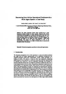
3. Task Description The focus of our investigation is an industrial facility [1]. This production cell comprises six physical components: two conveyor belts, a rotatable robot equipped with two extendable arms, an elevating rotary table, a press, and a travelling crane. The machines are organised in a (closed) pipeline (see Fig. 2). Their common goal is to transport and transform metal blanks. The production cycle of each blank is as follows: the feed belt conveys the blank to an elevating rotary table. The table rotates and rises to position the blank where the first robot arm is able to grasp it. The robot fetches the blank from the table and places it into the press. After it is processed, the second robot arm places the blank on the deposit belt. A travelling crane is added to the model to ensure a permanent supply by transporting the blank back to the feed belt and making the model self-contained. The devices are now described in more detail. Feed Belt and Deposit Belt. Both belts are powered by an electric motor which can be started or stopped by a control program. A photoelectric cell installed at the end of each belt indicates whether a blank has entered the final part of the belt. In both cases, a blank must leave the photo cell’s control area. In that position the blank drops from the feed belt onto the table, while the crane is able to pick up a blank in similar position from the deposit belt. 1. Elevating Rotary Table. Both vertical movement and rotation of the table are necessary. The first robot arm is located at a

A Case Study in Design and Verification

Fig. 1. Tool overview.

141

142

M. Heiner et al.

Fig. 2. Top view of the production cell.

different level to the feed belt and is unable to perform a vertical translation. Furthermore, the arm grippers (electromagnets) are not rotatable and are not able to place a blank in an appropriate angle into the press by themselves. An analog potentiometer indicates the rotation angle of the table. Boolean valued switches are activated when the table reaches its top and bottom positions, respectively. 2. Robot. The robot consists of two extendable arms, mounted orthogonally at different levels, and a swivel for rotation. To grasp a blank from the table and the press, respectively, the arms must be extended. In order to meet various safety requirements, each arm has to be retracted while the robot rotates or the other arm loads or unloads a blank. The extensions of the robot arms and the rotation angles are indicated by potentiometers. 3. Press. The press forges metal plates by pressing its lower plate against the upper plate. Because of the placement of the robot arms at different horizontal levels, the lower plate of the press is movable into two other positions: a middle position for loading by the first arm and a lower position for unloading by the second arm. In the upper position a blank is forged. Switches signal the position of the lower plate of the press. 4. Crane. The task of the crane is to transport metal plates from the deposit belt back to the feed belt to ensure a permanent supply of blanks without involving any further external components. Its gripper (an electromagnet) is movable in the horizontal and vertical directions. After the gripper has picked up a blank, it lifts, performs a horizontal movement

back to the feed belt, and lowers to release the blank. The sensor set of the crane comprises switches, which are activated if the gripper is positioned above one of the belts, and a potentiometer which indicates the height of the gripper. Altogether, there are 14 sensors and 34 actuators in the production cell. Additionally, various safety requirements are given in [1] which are to be obeyed by an implementation of the controllers for the production cell. These requirements are consequences of restrictions of the machine’s mobility and the danger of damage caused by the possible collision of several machines. Another safety requirement is that the controllers have to make sure that metal blanks are not dropped outside intended areas. We give two examples: 1. Avoidance of Machine Collisions. For instance, a collision between the press and the robot is possible. One requirement is that the press must close only when no robot arm is positioned inside it. 2. Blanks are not Dropped Outside Safe Areas. For instance, a metal blank would be dropped if the electromagnet of a robot arm is deactivated before the device reaches its designated unloading position.

4. Modelling with Hierarchical Petri Nets For the description of the control program of the production cell we use ordinary, hierarchically organised place/transition


nets without extensions such as priorities or place capacities. Readers not familiar with the basic notions of Petri net theory are referred, for example, to Peterson [19]. 4.1

General Procedure

The control software was developed and analysed stepwise at two abstraction levels (see Fig. 3) constituting the cooperation model (see Section 4.2) and the control model (see Section 4.3). The more abstract cooperation model describes the synchronisation of the machine controllers. The construction of the model was carried out bottom-up in the following way. First, (three) general reusable patterns concerning the intended communication behaviour of the controllers for the physical devices were identified and modelled as Petri nets (communicating state machines) inspired by Casais [20]. These communication patterns were analysed. Then, the complete model was constructed by composition of instances of these communication patterns via merging so-called communication places. After having analysed the cooperation model successfully, refinements (of places as well as of transitions) were made by modelling the interactions of the controllers with the hardware interface (actuators, sensors) of the production cell. Furthermore, this control model comprises a Petri net description of the environment, i.e. the controlled plant. As before, the construction of the model was carried out bottom-up. A general

143

net structure for an elementary control procedure was identified, which involves the controller part as well as the environment part, of one basic motion step of any device type. More complex processing step controls were constructed by combining elementary ones. After having modelled and analysed the refined controllers separately, the control model was composed as described above. It is worth noting that the whole net has been constructed systematically using extensively a very small set (seven) of reusable components. Therefore, similar control applications can be configured efficiently in a very short time period. The total net, which can be found in Heiner and Deussen [21], consists of 231 places and 202 transitions structured into 65 nodes of the hierarchy tree. 4.2 Cooperation Model

The manufacturing system considered consists logically of seven loosely coupled machine controllers acting largely independently of each other. These machine controllers are organised in a (closed) pipeline to realise the transportation/transformation of the metal plates. For that purpose, neighbouring machine controllers communicate with each other according to a synchronous producer/consumer relationship. There is neither a central controller of the production cell responsible for activating and deactivating the machines,

Fig. 3. Bottom up design and analysis.

144

M. Heiner et al.

nor a global observer with full knowledge of the total state of the production cell and of the metal plates. Each machine follows a similar operation pattern: fetch a metal blank from the input region, process it, and deposit the plate on the output region. In order to do that, each machine performs cyclically a certain sequence of motions (synchronised according to the states of its neighbours). If two machines are connected, the output region of the predecessor, and the input region of the successor, merge to a cooperation region between two consecutive machines. Such a cooperation region has to be organised as a mutual exclusion region, i.e. either the predecessor is allowed to put a plate into the region, or the successor has the access rights to take a plate from the region. However, the concurrent access to the cooperation region by the adjacent machines is forbidden. Furthermore, owing to the given machine equipment, a cooperation region does not have any buffering capabilities. So the predecessor is allowed to put a plate into the region, only if the region is free, and the successor can take a plate from the region, only if it is full. Figure 4 shows the elementary relationship of each controller to the controllers of neighbouring machines. The input and output regions of the controller are modelled by the four grey-shaded places. According to the mutual exclusion requirement for the cooperative regions of consecutive machines, each controller has to make sure that at most one token is placed at both of its input region places, and analogously, at most one token is placed at both its output region places. Additionally, there are two kinds of mutually exclusive shared resources. The robot arms are organised separately to enlarge the possible degree of parallelism within the production cell (which may possibly result in a higher throughput). In doing so, the robot swivel (the engine to rotate both arms), becomes a shared resource of the arms, which can be used only exclusively. There exist shared physical regions (intersection of trajectories of different machines). To avoid machine collisions, such shared physical regions have to be used exclusively. In our case study, the trouble disappears in a constructive way, by the ad hoc requirements that the robot arms and the crane are allowed to move only if they are retracted and lifted, respectively. Let us have a closer look into the controllers. There are three basic types of communication pattern according to the order in which input and output regions are acquired and released (see Fig. 5). (Please note the following drawing convention. Grey-shaded nodes are so-called fusion nodes. They serve as connectors: all fusion nodes with the same name are

logically identical. Therefore, they will be merged physically for the analysis data structures. Usually, communication objects are represented by such fusion nodes to avoid immoderate edge crossing.) 1. Independent input/output. For the next operation cycle, the controller has to synchronise with only one of its adjacent controllers, e.g. to take a plate from the input area, a free output area is not required and vice versa. This pattern is applied to the arms and the crane. 2. Dependent input/output. For the next operation cycle, the controller needs simultaneous control of input and output regions. This pattern is very useful to control the belts in such a way that the plates remain distinguishable. A belt is switched on only if a new plate has arrived (input available) and the output area is free. So at any time, a maximum of two plates can be on the belt – one at each end of the belt. 3. Mutually exclusive input/output. At any time, the controller must hold a lock on one of its cooperation regions, i.e. the output region can only be released after having locked the input region and vice versa. This pattern is used for machines such as the table and the press, which cannot be in a position suitable for loading as well as unloading at the same time. Now let us consider the arms in more detail. First, they follow the independent input/output cooperation pattern. Secondly, both arms have to be synchronised in order to use the swivel only in a mutual exclusive manner. These two basic synchronisation patterns have to be combined in an interleaving way. Three possible arm versions are shown in Fig. 6. In version 1, the preconditions to start a motion step are acquired simultaneously. To implement this behaviour, corresponding compact language primitives are required which are usually not available in implementation languages. Alternatively, arm version 2 and 3 correspond in a straightforward manner to the program sketches in Fig. 7 [20]. The control system of the production cell is composed of the machine components just introduced. The coarse structure given in Fig. 8 provides an overview of the whole (closed) system. It shows the top level of a hierarchically structured Petri net which is the result of the linking step. During linking, all (private) nodes of one controller are uniquely prefixed to preserve node name uniqueness within the total system. Each of the macro transitions (represented as nested double boxes) includes the behaviour of one controller on the next lower level (i.e. the net structures of Figs 5 and 6, but with prefixed node names).

4.3 Control Model

Fig. 4. Producer consumer relation.

In order to be able to express safety requirements referring to physical devices, the controllers’ net models have to be extended by a net description of the environment reflecting all essential assumptions about its behaviour. The environment model for each physical device is divided into two parts: an actuator model, which describes the possible


145

Fig. 5. Three types of communication pattern.

Fig. 6. Three arm versions.

Fig. 7. Source test examples [20].

states of a device and a sensor model, which expresses the sensor values which must be received by the controller (see Fig. 9). Actuators (e.g. the press’ engine) are effected by commands (e.g. press upward, press stop, press down). We can identify the states of each device with the commands to control them (so for the press, there exist three possible states). A net description of the actuator states is obtained by adding a place PA for each command A. A marking of PA with one token means that the corresponding device has received the command A and is in an associated state.

146

M. Heiner et al.

Fig. 8. Coarse structure of the closed system.

A controller performs actions in response to specific (discrete) sensor values. To construct an environment model, when describing the relations between sensors and actuators, it is enough to represent in the model, only those finite discrete sensor values, out of the whole set of generally analogous values, which may cause a reaction of controllers (e.g. press at lower pos, press at middle pos, press at upper pos). A net description of the relevant sensor states of the production cell is obtained by adding a place PV for each of these values V. PV is marked with one token if the value V is received by the control program. Let us now discuss in more detail the model of the controller’s interactions with the environment. Every complex control action is decomposed into elementary motion steps (like press forge, press lift, etc.). One such step consists of device activation (start command), waiting for a certain sensor value indicating that the motion has been completed (wait stop con(dition)), and device deactivation (stop command) (see the lefthand side of Fig. 9(a)). A start command will force the associated device to change from an inactive to an active state. A stop command is assumed to force the device to change to an inactive state. The net in Fig. 9(a) (righthand side) (actuator state model) shows the modelling of these assumptions. The places stop command and start command represent the actuator states corresponding to the deactivation and activation of the actuator, respectively. Each elementary motion step is performed in the context of an initial sensor value indicating the current position of the corresponding device. It is assumed that the performed motion will eventually cause the occurrence of a certain final sensor value. The places start con(dition) and stop con(dition) represent the initial and final values of the sensor state model. The transition css (change sensor state) implements this assumption (see Fig. 9(a) righthand side, sensor state model). To increase readability, control procedure and environment descriptions are abstracted by a macro component (coarse node with interface places), as shown in Fig. 9(c). Instantiating the macro net involves renaming of formal parameter places by

Fig. 9. Petri net component of basic motion step and environment (from top to bottom). (a) Basic models. (b) Composition of the 3 models in Fig. 9(a). (c) Macro component of Fig. 9(b) (with formal parameters).

actual parameters. The total net comprises 37 instances of this basic macro, forming the sheets of the hierarchy tree.

5. Qualitative Analysis Owing to the lack of applicable compositional Petri net analysis approaches, all analytical results have to be confirmed after each refinement/composition step. However, it is a widely accepted engineers’ basic principle that a sound composition/ refinement has to be based on sound components. So, the successful analysis of a given model at a certain abstraction level is considered to be a necessary (but unfortunately not sufficient) condition to go ahead in modelling. In this way, design faults can be detected early.


5.1

General Analysis

For the cooperation model, general analysis was carried out successfully using INA. Boundedness and liveness could be decided efficiently (i.e. without construction of the complete reachability graph) by showing that the net is covered by semipositive place invariants and by proving the deadlock trap property (in connection with the net structure Extended Simple), respectively. Dead states caused by one controller version (arm version 2) have been found very fast by construction of the (surprisingly small) stubborn set reduced reachability graph. Table 1 summarises some of the steps carried out for the analysis of the cooperation model. For comparison, we also tried to apply OBDD-based methods. OBDDs represent the set of reachable states of a system by its characteristic function, that is a Boolean function in the number of variables necessary to describe a system state. The efficiency of OBDD based methods depends critically on the ordering in which these variables occur. Table 2 collects some execution times and storage uses measured in the number of OBDD nodes necessary to represent the states spaces to decide the liveness of the considered subsystems of the cooperation model. Note the effect of using a formerly computed variable ordering.

For the control model, boundedness can still be decided very quickly by showing that the net is covered with semipositive place invariants. Owing to the added environment behaviour, all net models exhibit a net structure beyond the Extended Simple one. So, the deadlock trap property could only show the freedom of dead states. However, this can be proved more efficiently by constructing the stubborn set reduced reachability graph (even for the completely refined open system with a still unknown state space size). Because of the very large size of the state space of the control model, the time and space effort to generate the complete reachability graph (to prove, for example, liveness) became unmanageable. Like many other “classical” net properties, the liveness property can also be expressed by a set of CTL formulae (one for each transition, see next section). However, because their evaluation relies on the complete reachability graph, PROD’s CTL model checking component (which is based merely on graph traversing strategies and evaluation of state expressions) is not applicable in the case of the control model. The evaluation of an LTL formula may be based on a stubborn set reduced reachability graph, resulting generally in much smaller sets of reachable states. However, in LTL, only a stronger liveness property of transitions can be expressed,

Table 1. Size of analysed nets and analysis efforts using INA and PROD (cooperation model). Subsystem

Places/transitions

Analysis (INA) DTPa

Execution times (s)

Rstubb

Rc

INAd

INAe

PRODf

Controllers Table/press with init part without init part

13/9 12/8

– 28

12 8

28 24

1.5 1.46

1.54 2.16

7.96 7.41

Crane

12/8

31

11

48

1.62

2.12

7.39

Arm version 1 version 2 version 3

13/8 17/12 17/12

38 109 88

11 15 15

48 112 96

1.5 1.73 1.77

3.12 1.65 1.88

14.78 24.92 24.19

Belts

12/8

26

8

36

1.58

2.23

7.38

Robot (arm version 3)

33/24

448

221

6912

2190.18

11.34

75.6

Robot/press with arm version 1 arm version 2 arm version 3

25/16 33/24 33/24

175 3.851 725

47 75 140

640 1984 1800

7.81 53.23 57.07

3.64 7.78 8.12

14.78 24.92 24.19

Open system

51/36

1145

299

77 760

Closed with with with with with

51/36

1140 36 72 94 98 121

864 4776 12 102 16 362 12 144

Composed systems

a

system 1 plate 2 plates 3 plates 4 plates 5 plates

Processed candidates to check the deadlock trap property. Number of states of the stubborn reduced reachability graph Rstub. c Number of states of the complete reachability graph R. d Time effort to generate R (with coverability test). e Time effort to generate R (without coverability test). f Time effort to generate R. b

147

86 132.6 18.58 365.53 2401.28 4167.93 2373.1

3653.6 6.07 18.77 87.1 150.85 78.6

1073.35 25.93 56.21 125.71 169.15 123.8

148

M. Heiner et al.

Table 2. Analysis of the model using SMV (cooperation model).

Subsystem

Without reordering

Computation of reordering

With reordering

Time (s)

Time (s)

Time (s)

BDD nodes

BDD nodes

BDD nodes

Controllers Belt

0.10

3962

0.12

2762

0.04

3723

Table/press

0.09

2902

0.14

2149

0.12

2656

Crane

0.12

4075

0.16

2643

0.11

3555

Arm version 1 version 2 version 3

0.13 0.22 0.23

4270 10017 9735

0.18 0.29 0.35

2837 5073 5015

0.12 0.18 0.21

3720 9806 8816

Robot (arm version 3)

21.93

41685

1.00

7671

6.76

11829

Robot/press with arm version 1 arm version 2 arm version 3

1.88 11.02 13.38

10292 11231 15618

3.14 9.59 10.14

5799 6378 7012

1.08 8.93 6.10

10093 10680 10365

Open system

343.19

103319

205.03

31506

99.80

44732


36.29 77.14 144.89 182.46 275.53

48984 59467 94818 108414 180507

22.39 57.40 69.00 75.38 49.90

8357 12041 16847 20292 14906

13.58 23.48 37.10 54.06 30.41

11163 17662 27101 40188 12144

Composed systems


which is more related to the livelock freedom of transitions. On every infinite computation path, a transition is enabled infinitely often. Every strongly live transition is also live. This formula was checked for every transition in the control model using a batch program. However, the formula does not hold for all transitions in the control model (as expected, any actions in alternative execution branches are not strongly live). For these remaining transitions we succeeded in proving liveness using the model checker of the PEP tool (see next section for a comparison of the expressive power of the temporal logics supported by the different tools). The analysis steps concerning the control model are summarised in Table 3. There are some success stories about OBDD based methods in the literature (for SMV, see e.g. [22] or [23]). However, the SMV system proved to be inapplicable for the validation of the control model. We were only able to generate the OBDD representation of the state space of very small system components comprising only one controller. For instance, even the analysis of a system comprising the two robot arm controllers (just 63 232 states) was stopped after several hours run time and the construction of only a few hundred states. However, it should be noticed that SMV is not designed for the analysis of Petri net models. Although the structure and dynamic of Petri nets can be expressed in SMV’s input language, an implementation of an OBDDbased model checker, dedicated especially to Petri nets, might produce much better results.

5.2 Special Analysis

To highlight the difference between the applied tools concerning their expressiveness, it is useful to summarise typical questions/properties dealt with during special analysis. In the following formulation, ␸ denotes a general logical expression characterising usually a (wanted or unwanted) state or set of states. 1. Reachability-related (reachability of a state where ␸ holds): EF␸ (There exists at least one computation path (future behaviour) to reach eventually a state where ␸ will be true.) 2. Safety-related (unreachability of a state where ␸ holds): AG (G␸),

(equivalent to GEF␸)

(For every computation path, ␸ will never be true.) 3. Invariant-related (general validity of an assertion ␸): AG ␸, (equivalent to GEF (G␸)) (For every computation path, ␸ will be true for ever.) 4. Liveness-related: AG EF␸ (Whatever happens, there exists the chance (at least one path) that ␸ will be true.)


149

Table 3. Size of analysed nets and analysis efforts using PEP and PROD (control model). Subsystem

Places/transitions

PEP Conditions/ eventsa

PROD Timeb (s)

Rc

Timed (s)

Rstube

Timef (s)

Rstubg

51

0.16

38

Timeh (s)

Controllers Crane

45/34

14/71

0.02

256

0.78s

0.08

Feed belt

22/16

69/34

0.01

69

0.20s

31

0.10

16

0.07

Table

32/24

82/37

0.01

88

0.38s

36

0.15

24

0.09

Arm (version 3)

66/60

138/65

0.02

365

1.19s

62

0.23

51

0.09

Press

28/20

166/81

0.02

140

0.42s

48

0.10

20

0.09

Deposit belt

22/16

69/34

0.01

69

0.20s

31

0.11

16

0.07

Robot

124/120

3514/1752

0.02

63 232

11.26s

992

5.99

205

0.21

Robot/press

140/132

1280/624

1.07

18 344

3.10s

557

3.46

305

0.35

Open system

198/176

2773/1348

5.15

?

798

5.90

507

0.62


231/202 690/316 1670/792 2009/960 2164/1035 1619/768

0.57 2.63 3.02 3.38 1.68

162 406 523 471 585

0.68 2.53 4.51 4.02 5.05

163 456 635 678 608

0.32 0.72 0.95 1.06 0.98

Composed systems


30 952 543 480 >1.7 Mio >3.1 Mio 1 657 242

? 7.54 Ca. 3.3 h >20 h >42 h ca. 14 h

a

Size of the finite prefix of the branching process (net unfolding). Time effort to generate the finite prefix. c Number of states of the complete reachability graph R. d Time effort to generate R. e Number of states of the stubborn reduced reachability graph Rstub using the deletion algorithm. f Time effort to generate Rstub. g Number of states of the stubborn reduced reachability graph Rstub using the incremental algorithm. h Time effort to generate Rstub. b

5. Progress-related: AG AF ␸ (For every computation path, ␸ will eventually be true.) Which tools may be applied at all for a given type of question depends on the temporal logic it provides. Table 4 gives a comparison of the model checkers in use and the versions of logics provided. Which tools should be applied in which order depends on the analytical methods they are based on. The analyses of PEP are based on a so-called finite prefix of a branching process [13,24,25]. In the case of concurrent

systems with a moderate amount of non-determinism, these graphs are much smaller than the “classical” complete reachability graphs because they alleviate the state explosion by avoiding the enumeration of all interleaving combinations for independently concurrent actions. PROD uses stubborn set reduced reachability graphs, which are generally, in the case of highly concurrent systems, much smaller than the complete reachability graph. Such a reduced (very small) graph is newly constructed for each LTL question. We succeeded in constructing stubborn set reduced versions of the reachability graph as well as of the finite prefix of branching processes, even for systems for which total system state size is still not known.

Table 4. Comparison of tools and supported temporal logics. Tool

Supported type of logic temporal

Operators

Type of properties expressible

INA (version 1.7)

–

EF ␸ (but ␸ can only be given by a (sub-) marking) (1), (2)

PEP

(restricted) CTL

AG, EF

(1)–(4)

PROD

LTL (without next-time operator)

G, F, U (unquantorized versions of AG, AF, AU)

(2), (3), (5)

PROD SMV

(full) CTL

EX/AX, EU/AU, EF/AF, EG/AG

(1)–(5)

150

M. Heiner et al.

Because the evaluation of PROD’s CTL relies on the complete reachability graph, its application should be tried only if the formerly mentioned methods did not help. In our experience, the same seems to be true for SMV. This helpful meta-knowledge of the tool’s internal analysis techniques should be provided to the tool box users, e.g. by a dialogue-oriented user guideline of the Petri net framework implementation (see Fig. 1). Altogether, about 25 different requirements of the cooperation model expressed by CTL and of the control model expressed by LTL have been proved successfully. The following examples demonstrate the variety: 1. Reachability-related, e.g.: To gain deeper insight into the controllers’ concurrency: Is it possible that both robot arms hold a plate at the same time? EF (arm1 mag on ⵩ arm2 mag on) 2. Safety-related, e.g. those properties mentioned in Section 3. In particular: The press may only be closed, if no robot arm is positioned inside it, i.e. for arm 1: G ((arm1 release angle ⵩ arm1 release ext) → (press stop ⵩ +press at upper pos)) If arm 1 is loaded (its magnet is activated), it remains loaded until it reaches its unloading position. G ((arm1 pick up angle ⵩ arm1 pick up ext ⵩ arm1 mag on) →(arm1 mag on U (arm1 release angle ⵩ arm1 release ext))) Note that the until operator U is required to express this property. 3. Invariant-related, to prove design consistency, e.g. The press is either stopped or moves in exactly one direction, i.e. it is always in one of its actuator states: · press upward ⵪ · press down) G (press stop ⵪ · denotes exclusive disjunction.) (⵪ The press is always positioned (logically) at exactly one of its sensor states: · press at middle pos ⵪ · G (press at lower pos ⵪ press at upper pos) 4. Liveness-related, e.g. a Petri net transition t is live iff it may be enabled infinitely often: AG EF ⵩ p˜ p苸앫t

(A transition t of an ordinary Petri net is enabled (may fire) if all its preplaces hold a token (here p˜ denotes the interpretation of a place name as an atomic proposition: p˜ holds true if p is marked with one token at a state where the proposition is evaluated. As usual, 쐌x denotes the set of predecessor nodes of a net element x (place or transition), and x쐌 stands for the

set of its successor nodes. An analogous notation applies to sets of net elements). 5. Progress-related, e.g. a transition t is strongly live iff it will be enabled infinitely often: AG AF ⵩ p˜ p苸앫t

The necessary analytical efforts for model checking of these requirements may be summarised in the following way. PROD’s stubborn set based evaluation method of LTL formulae has been proven applicable even for medium-sized systems. (The sizes of the stubborn set reduced reachability graphs constructed to evaluate formulae like those given above have been between 500 and 30 000. The time efforts were between 2 and 25 min on a SPARC Station 20.) However, livenessrelated properties cannot be expressed in LTL because of the lack of quantification for computation paths. On the other hand, PROD’s model checker for full CTL formulae is not applicable for the control model because it depends on the complete construction of its state space. Surprisingly good results are gained by using PEP’s model-checking algorithm for the verification of liveness-related, as well as safety-related, properties. (Liveness of transitions, for instance, can be checked in an insignificant amount of time (0.04 s). Similar results are obtained for simple safety formulae of type 2 (see above). The finite prefix of the control model consists of 1619 conditions and 768 events, constructed in less than 0.1 s on a SPARC Station 20.) Therefore, the model-checking techniques provided by PEP and PROD seems to be a suitable combination in the context of our application area.

6. Synthesis In order to avoid any additional implementation faults, the actual control software has been directly synthesised from the Petri net specification in the following way: for the simulation (animation by playing the token game) of the Petri net, a very small Petri net simulator (FUNlite) has been realised, designed especially for the fast execution speed and low memory consumption. (The source code of the FUNlite execution kernel has a size of 50 lines (including comments) which results in 5 kB of object code on a SPARC Station 20.) FUNlite is currently restricted to 1-bounded Place/Transition nets, but could be easily extended to bounded Place/Transition nets (as long as the capacities of the places are known). When simulating a Petri net, by playing the token game, the speed of the transition enabling test plays an important role. In FUNlite the enabling test is highly simplified by a method characterising the enabling of a transition at a given marking by a simple number comparison. For each transition a counter is introduced which characterises the firability of that transition. The counter of a transition t shows the number of unmarked preplaces of t. If the counter of a transition t decreases to 0 the transition gets enabled. After the firing of a transition t, we have only to consider the transitions sets (쐌t)쐌 and (t쐌)쐌. For each transition t⬘ in (쐌t)쐌, the counter of t⬘ is increased by the number of common preplaces with transition t. For each transition t′ in (t쐌)쐌, the


counter of t′ is decreased by the number of common places between the preplaces of t⬘ and the postplaces of t. For more information about extending this method to structurally bounded Place/Transition nets, see [26]. Based on the FUNlite Petri net simulator, a FUNlite description of the total net structure and a C-procedure skeleton for each transition was automatically generated. There are 37 basic macro transitions, containing the elementary motion steps. For the three transitions of all these basic macros (start command, wait stop con, stop command, see Fig. 9(b)) the corresponding procedure skeleton had to be filled with the actual elementary motion code. The remaining transitions simply play the token game. The assignment of all these procedures to the corresponding transitions is handled by name equivalence. The procedures are executed if the corresponding transition fires. All elementary motion code declarations are local to their Cprocedure skeletons. This prevents destruction of the wellanalysed net behaviour. Therefore, any (implicit) communication between these procedures has been made impossible. The generated control software runs in a graphical simulation environment of the production cell implemented with Tcl/Tk on UNIX computers. The communication between the control software and the simulation environment follows a simple ASCII-based input/output protocol. Therefore, the elementary motion code consists of simple I/O statements. The example in Fig. 10 illustrates the syntactical structure of an elementary motion step procedure (corresponding to the start command of the basic macro transition to extend arm 1 from the retract position to the pick-up position). There are two parts. One part represents the automatically generated procedure skeleton (plain), and the other one contains the included elementary motion code (bold). The control software was compiled for two different machine types, for SUN workstations and for a T9000 based distributed multiprocessor architecture. In the later version, each controller runs on its own processor. As a welcome (but not surprising) confirmation of our general approach, both versions run, after successful compilation, right from the beginning without any trouble.

7.

Conclusions

To date, a Petri net model to control the given production cell has been developed which enjoys provably a lot of valuable qualitative properties – general as well as special ones. The following investigations are in progress:

Fig. 10. FUNLite transition code.

151

Worst-case evaluation by duration interval nets introduced in [27] (firing of transitions consumes time characterised by interval delays) to prove the meeting of given deadlines (implemented in the latest update of INA). Quantitative analysis of stochastic nets [28] for performance and reliability evaluation. Incorporation of fault tolerance aspects (blowing up the net sizes significantly). Throughout this paper, (the rarely available and rather restrictive) compositional approaches of Petri net analysis have not been discussed. They have been omitted in order to concentrate on the borders of those net/state space sizes, which are manageable by available analysis tools. Finally, the main lessons learnt concerning a suitable tool box framework are the following: The combination of different tools (even if they provide similar features at the first glance) seems to be unavoidable. User guidelines showing which analysis techniques are to be recommended for a given analysis question are needed. The check of a given system against its functional and/or safety requirements given by a (more or less large) set of temporal formulae calls for distributed evaluations in batch processing operation mode. Acknowledgements

We are grateful to Claus Lewerentz for drawing our attention to the production cell case study. We thank Peter H. Starke, Bernd Grahlmann, Kimmo Varpaaniemi, and especially Guido Wimmel for their assistance in using their tools.

References 1. C. Lewerentz and T. Lindner, Formal Development of Reactive Systems – Case Study Production, Lecture Notes in Computer Science, 891, Springer, 1995. 2. M. Heiner, Petri Net Based Software Validation, Prospects and Limitations, ICSI-TR-92-022, Berkeley/CA, 1992. 3. M. Heiner, “Petri net based software dependability engineering”, Tutorial Notes, International Symposium on Software Reliability Engineering (ISSRE ’95), Toulouse, October 1995. 4. M. Heiner, G. Ventre and D. Wikarski, “A Petri net based methodology to integrate qualitative and quantitative analysis”, Journal of Information and Software Technology, 36(7), pp. 435– 441, 1994. 5. “ PED – a hierarchical Petri net editor ”, http://www-dssz. Informatik.TU-Cottbus.DE/~wwwdssz 6. H. P. Starke, INA – Integrated Net Analyser, Manual (in German), Berlin 1992 (see also http://www.informatik.hu-berlin.de/~starke/ ina.html). 7. K. Varpaaniemi, J. Halme, K. Hiekkanen and T. Pyssyslao, PROD Reference Manual, Helsinki University of Technology, Digital Systems Laboratory, Series B: Technical Report no. 13, Espoo 1995 (available at http://saturn.hut.fi/~petrinet/publications.html). 8. M. Ben-Ari, M. A. Pnueli and Z. Manna, “The temporal logic of branching time”, Acta Informatica, 20, pp. 207–226, 1983. 9. E. A. Emerson, “Temporal and modal logic”, in: J. van Leeuwen (ed.), Handbook of Theoretical Computer Science, vol. B, Elsevier, Amsterdam, pp. 995–1072, 1990. 10. A. Valmari, “Alleviating state explosion during verification of behavioral equivalence”, University of Helsinki, Department of

152

11. 12.

13. 14. 15. 16. 17.

18. 19. 20.

M. Heiner et al. Computer Science, Report A-1992-4, Helsinki 1992 (available at http://saturn.hut.fi/~petrinet/publications.html). A. Valmari, “A stubborn attack on state explosion”, Formal Methods in System Design, 1(4), pp. 297–322, 1992. E. Best and B. Grahlmann, PEP – Programming Environment Based on Petri Nets, Documentation and User Guide, University of Hildesheim, Department of Computer Science, November 1995 (available at http://www.informatik.uni-hildesheim.de/~pep). J. Esparza, “Model checking using net unfoldings”, Science of Computer Programming, 23, pp. 151–195, 1994. K. L. McMillan, The SMV System, Technical Report, CarnegieMellon University 1992 (available at http://www.cs.cmu.edu/ ~modelcheck/smv.html). K. L. McMillan, Symbolic Model Checking, Kluwer, 1996. R. E. Briant, “Graph-based algorithms for Boolean function manipulation”, IEEE Transactions on Computers, C–35(8), pp. 677–691, 1986. R. German et al., TimeNet – A Tool Kit for Evaluating NonMarkovian Stochastic Petri Nets, Technical University of Berlin, Department of Computer Science, Report 1994-19 (see also: http://pdv.cs.tu-berlin.de/forschung/timenet.html). J. Spranger, “FUNLite – A parallel Petri net simulator”, Proceedings 42nd IWK, Technical University Ilmenau, pp. 563–568, 1997. J. L. Peterson, Petri Net Theory and the Modeling of Systems, Prentice-Hall, Englewood Cliffs, NJ, 1981. E. Casais, “Eiffel: A reusable framework for production cells developed with an object-oriented programming language”, in C. Lewerentz and T. Lindner (ed.), Case Study “Production Cell”

21.

22. 23. 24. 25.

26. 27.

28.

A Comparative Study in Formal Software Development, FZIPublication 1/94, Forschungszentrum Informatik, Karlsruhe, pp. 241–256, 1994. M. Heiner and P. Deussen, Petri Net Based Qualitative Analysis – A Case Study, Brandenburg Technical University of Cottbus, Department of Computer Science, Technical Report I-08/1995 (available at http://www-dssz.Informatik.TU-Cottbus.DE/~wwwdssz). J. C. Corbett, Evaluating Deadlock Detection Methods, Technical Report, University of Hawaii at Manoa, 1994. S. T. Probst, Chemical Process Safety and Operability Analysis Using Symbolic Model Checking, PhD Thesis, Carnegie Mellon University, Department of Chemical Engineering, 1996. J. Engelfriet, “Branching processes of Petri nets”, Acta Informatica, 25, pp. 575–591, 1991. K. L. McMillan, “Using unfoldings to avoid the state explosion problem in the verification of asynchronous circuits”, Proceedings, 4th Workshop on Computer Aided Verification, Montreal, pp. 164– 174, 1992. J. L. Briz and J. M. Colom, “Implementation of weighted place/transition nets based on linear enabling functions”, Lecture Notes in Computer Science, 815, Springer, pp. 99–118, 1994. M. Heiner and L. Popova-Zeugmann, “Worst-case analysis of concurrent systems with duration interval Petri nets”, in E. Schnieder and D. Abel (eds.), Proceedings 5th EKA ’97, Braunschweig, pp. 162–179, 1997. D. Wikarski and H. Heiner, On the Application of Markovian Object Nets to Integrated Qualitative and Quantitative Software Analysis, Fraunhofer ISST, Berlin, ISST-Berichte 29/95, 1995.