A Case Study in Performance-Oriented DSL ... - Infoscience - EPFL

StagedSAC: A Case Study in Performance-Oriented DSL Development Vlad Ureche

Tiark Rompf

EPFL {first.last}@epfl.ch

Arvind Sujeeth

Stanford University {asujeeth,hchafi}@stanford.edu

Abstract Domain-specific languages (DSLs) can bridge the gap between high-level programming and efficient execution. However, implementing compiler tool-chains for performance oriented DSLs requires significant effort. Recent research has produced methodologies and frameworks that promise to reduce this development effort by enabling quick transition from library-only, purely embedded DSLs to optimizing compilation. In this case study we report on our experience implementing a compiler for StagedSAC. StagedSAC is a DSL for arithmetic processing with multidimensional arrays modeled after the stand-alone language SAC (Single Assignment C). The main language feature of both SAC and StagedSAC is a loop construction that enables high-level and concise implementations of array algorithms. At the same time, the functional semantics of the two languages allow for advanced compiler optimizations and parallel code generation. We describe how we were able to quickly evolve from a pure library DSL to a performance-oriented compiler with a good speedup and only minor syntax changes using the technique of Lightweight Modular Staging. We also describe the optimizations we perform to obtain fast code and how we plan to generate parallel code with minimal effort using the Delite framework. Categories and Subject Descriptors niques]: Automatic Programming General Terms

Hassan Chafi

D.1.2 [Programming tech-

Experimentation, Languages, Performance

Keywords Staging, DSL, Domain Specific Languages, Optimization, SAC, Single Assignment C

1. Introduction Developing compilers for performance-oriented domain specific languages (DSLs) is a complex undertaking. DSLs form bridges between high level programs and low level machine code, so their development requires an in-depth understanding of both sides and how they map to each other. Generating fast programs also requires careful optimization at both ends, as both high-level and lowlevel representations present their own unique optimization opportunities. In addition to this, the inherent complexity of a compiler makes development a hard, costly and time consuming undertak-

Permission to make digital or hard copies of all or part of this work for personal or classroom use is granted without fee provided that copies are not made or distributed for profit or commercial advantage and that copies bear this notice and the full citation on the first page. To copy otherwise, to republish, to post on servers or to redistribute to lists, requires prior specific permission and/or a fee. PEPM’12, January 23–24, 2012, Philadelphia, PA, USA. c 2012 ACM 978-1-4503-1118-2/12/01. . . $10.00 Copyright 

Martin Odersky EPFL {first.last}@epfl.ch

ing. In this context we are looking at techniques that alleviate the burden of compiler development. An alternative to implementing DSLs from scratch as a standalone tool chain is to embed them into a general-purpose host language. This comes at the cost of losing many useful optimizations as the program’s structure is no longer available for analysis and manipulation. Recent research produced methodologies [7] and frameworks [22] that promise to significantly lower the development effort. In this paper, we report on our experience developing a multidimensional array DSL embedded into the programming language Scala using the technique of Lightweight Modular Staging (LMS) [21] and the Delite compiler framework [6]. The language and compiler we are studying is inspired by Single Assignment C (SAC) [24], a language which features a wellchosen set of high-level operations, enabling functional, concise and high-level programs for manipulating multidimensional arrays. The SAC compiler then transforms the programs into very fast lowlevel code that runs in parallel. Using Lightweight Modular Staging (LMS) and Delite, we were quickly able to switch from a pure-library embedding to an optimizing compiler. We began our development by building a purely embedded DSL, which we call LibrarySAC. LibrarySAC is basically just a Scala library and, since it does not perform any optimization, is very slow. Lightweight modular staging allowed us to transform LibrarySAC into a complete compiler with only minor changes to the DSL syntax. The core idea of using LMS is that as the program is executed, the library calls it makes are transformed into an intermediate program representation. Therefore the LMS framework lifts the entire program representation and allows the compiler to perform optimizations on it. Furthermore, along with the Delite parallel execution framework, it automatically simplifies the code by performing: • common subexpression elimination, constant folding, dead-

code elimination • code motion, loop invariant code hoisting (coarse grained, can

change the order of loops) • task parallelism (using the Delite framework, data parallelism

is ongoing work) The SAC compiler contains multiple optimizations that can significantly improve performance. Most of these optimizations rely on compile time information about the sizes of the arrays, also called array shapes. In SAC, the type system is augmented to infer array shape information, but it only performs top-down propagation and function inlining. We designed and implemented a new type system which is able to infer array sizes in a Hindley-Milner fashion, by deriving equations and solving them for a complete solution. Due to the nature of the language, for some programs it is impossible to infer complete array shape information. To overcome this limitation,

if the input files are available at compile time, we extract shape information and use it to specialize the program for the given input. Low level optimizations further improved performance. Our prototype compiler generates Scala code, which in turn is translated to Java Virtual Machine (JVM) bytecode. We performed several changes on the generated code to provide fast execution and we highlight our conclusions in Section 5. We use the Delite [6] framework, an extension to LMS that allows code to be executed in parallel on multiple CPUs and GPUs. The framework offers parallel abstractions to DSL authors, representing common execution patterns such as Map, Reduce, ZipWith, ForkJoin, etc. The code generated for these operations can be executed in parallel by the Delite runtime. It is worth noting that the parallel abstractions are only visible to the DSL author, making LMS and Delite languages indistinguishable to the DSL user. StagedSAC benefits from the Delite framework on two fronts: first of all, Delite enables parallel code generation for StagedSAC with very limited additional effort. Furthermore, as part of our current work, Delite will enable new optimizations that are present in SAC but were not yet available in StagedSAC. The optimizations are currently available for other DSL compilers [26], but need to be generalized to fit the case of the multidimensional arrays in StagedSAC. These optimizations will be further presented in Section 6. 1.1

Related Work

Given the wide applicability to modeling physical and statistical computations, a number of programming languages were proposed for efficient and high-level processing of multidimensional arrays [5, 8, 16, 17, 19, 24]. Each language features its own programming model, built-in array operations and restrictions. This makes the compilation and optimization very different for each language. Orthogonal to the means of obtaining fast array programs, significant effort went into developing each and every language and tool chain. This is where we hope the staging technique can alleviate the effort. The language chosen to evaluate the effectiveness of the staging technique is Single Assignment C [24], due to its shape-agnostic array objects, its expressive built-in operations and the numerous optimization techniques developed over the years. Therefore SAC met the two criteria for assessing whether the staging technique improves the state of art in DSL development: it has a performance-oriented compiler and several man-years went into developing the language and infrastructure. The StagedSAC language is heavily influenced by SAC [24]. Although the two languages are closely related, they are not exactly the same, as had to we adapt StagedSAC to be embedded in Scala [20] in order to use the LMS and Delite frameworks. In order to adapt the language for embedding, we had to drop axis control statements and rank notation in types [25]. Fortunately both can be simulated using additional code, so no language functionality was lost. On the compiler side the differences are drastic: the SAC compiler is a stand-alone application that translates SAC code to C and uses any C compiler to obtain machine code. StagedSAC on the other hand is embedded in Scala using the Delite framework and generates Scala code, which is later translated to JVM bytecode. Furthermore the set of optimizations in the two compilers are very different: some optimizations are only available in StagedSAC, as we will discuss in Section 5 while others [14, 15, 23] are only available in SAC. We are currently working on implementing more optimizations in StagedSAC by extending the Delite framework to support them in a generic fashion. The SAC compiler can speed up computation by targeting parallel architectures. It can produce code that runs in multithreaded environments [18] and on graphical processing units (GPUs). We added primitive support for parallel code generation in StagedSAC

using the Delite framework. As other domain-specific languages already showed [26], the Delite framework can enable optimizations that speed up DSL programs to the same performance as hand-tuned C code. We hope to obtain the same results for StagedSAC as part of our on-going work, adapting the generic Delite optimizations to StagedSAC arrays. Going one step further, the Delite framework supports interleaving execution on heterogeneous architectures. Previous experiments [22] show that the best execution speed is obtained by interleaving execution on different types of processors, either CPUs of GPUs, depending on the task. The Qube [27] compiler targets the same multidimensional array domain but aims at offering strong compile-time correctness guarantees. Qube compiles a modified subset of the SAC language and uses dependent types and SMT solvers to obtain complete array shape information. This benefits both safety and optimization, as many program manipulations require array size information at compile time. StagedSAC takes a more flexible approach: we use type inference and input specialization to obtain array sizes at compile time. Our approach does not guarantee full array shape information, but in practice it is enough to perform the optimizations, all without employing heavy machinery such as SMT solvers or completely redesigning the language and compiler, as in the case of Qube. The techniques used in developing StagedSAC are related to work in partial evaluation [13] and binding time analysis [9]. The Lightweight Modular Staging [21] framework encodes the dynamic or static nature of DSL expressions into types, thus offsetting the binding time analysis to Scala’s type system. The binding time analysis is thus performed as a single-pass, which is not always enough to detect all static expressions in the SAC language. Further refinement is performed in the shape analysis algorithm we developed. We improve on the SAC type system [24] and follow the formalization in [10]. We deliver a more fine-grained algebra of shapes, including partially known shapes, and introduce a different solving technique similar to Hindley-Milner unification [11]. The Repa system developed in Haskell implements optimizations typical to compilers at library level. The Repa system is standing proof that many of the optimizations available in multidimensional array languages can be implemented at library level. Repa relies on the Haskell type system and on programmer annotations to sidestep the lack of an entire program overview, while still being able to perform primitive loop fusion, data layout optimization and dead code elimination (by lazy evaluation). However, the staging technique can provide an overview of the entire program, as shown by the shape inference in StagedSAC, while at the same time requiring comparable implementation effort. By comparison to SAC, the array traversal operations in Repa are more coarse-grained thus easier to fuse together. SAC and StagedSAC provide more finegrained array traversal with bounds and strides, at the expense of more complex fusing algorithms and the necessity to perform shape inference. 1.2 Code Availability All the code for StagedSAC, the LMS framework and the Delite frameworks is available online, under open source license. The StagedSAC compiler [4] is built as one of the domain specific languages in the Delite repository [1], which itself relies on LMS [2] to function. 1.3 Paper Organization The rest of the paper is organized as follows: Sections 2 and 3 introduce the reader to multidimensional arrays and the operations provided by SAC. Section 4 reports our experience with the Lightweight Modular Staging framework while developing StagedSAC. Section 5 presents the optimizations in StagedSAC. Section

6 presents the Delite framework, parallel code execution and plans for future improvements. Section 7 presents the evaluation and Section 8 concludes.

2. Multidimensional Array Data Structure This section will present the multidimensional array data structure and will discuss some of the challenges of adding it to a language. First-class multidimensional arrays and powerful optimization algorithms are essential for compiling high-level and performanceoriented programs. In the rest of the paper we will use the following notation: arrays of dimension 1 are called vectors, arrays of dimension 2 are called matrices and arrays with more than 3 dimensions are called higher-dimensional. Furthermore, we’ll assume scalar values to be 0-dimensional arrays, we’ll use the term array to denote a multidimensional array with any number of dimensions and we’ll use the terms number of axes, rank or dimensionality to denote the number of dimensions. Accessing elements in a multidimensional array is done using integer index vectors of a length equal to the array rank. In the particular case of one-dimensional arrays, accessing elements is done using an integer vectors of 1 element. The common problem with accessing an element in either a vector or in any array is that the access must be made within the bounds of the allocated memory. To ensure this, multidimensional arrays introduce the shape vector containing the number of elements along each axis. The shape vector will always have a number of elements equal to the dimensionality of the array. In the case of an n-dimensional array with the shape vector s = [s0 . . . sn ], an index vector iv = [iv0 . . . ivm ] is valid if m = n and: ivi < si

∀0 ≤ i ≤ n

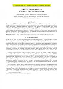
Selecting an index vector in a multidimensional array can also return an entire block. If the index vector contains less elements than the shape, m < n, instead of pointing to a value, it will point to an array of size t = [sm+1 , sm+2 , . . . sn ]. Figure 1 shows an array of shape s = [2, 3, 5]. Selecting the value at iv = [0, 1, 0] will produce the first element in the second row, a010 . Selecting the block at iv = [1, 0] will produce a vector of shape s = [5] which is highlighted in the figure.

ranks or shapes, so the more static information is available to the compiler, the faster code it can generate. In SAC and StagedSAC the layout chosen for multidimensional array data is a contiguous block of memory. This layout, coupled with data parallel operations, enables loop optimizations and parallel code generation. In the contiguous block layout, element access translates to computing an offset in the data block and accessing the element. Therefore the array shape is attached to the data and used to compute the memory block offset. Multiple shapes (with different dimensions) may fit in the same memory block, as long as the product of the elements in the shape vector is equal to the memory block’s size. (all of the shapes [3, 4], [2, 3, 2] and [12] will be correct for a block of size 12)

3. Single Assignment C This section presents the SAC language and compiler. It will only provide a brief overview of the most important operations in SAC in order to give enough background for the next sections. For a better understanding, the reader should consult the SAC tutorial [25] and the SAC journal paper [24] both of which present detailed descriptions and analyzes. 3.1 SAC Operations SAC is a functional restriction over the C language with first-class support for arrays. Multidimensional arrays are immutable data structures: once created their contents cannot be changed. Element updates create references to new arrays with the modified content. The same happens for shape changes, as the shape is intrinsically attached to the array. Making arrays immutable adds the referential transparency property but takes an important toll on memory and program speed. Since performance is a critical issue, the SAC compiler generates code that updates arrays in place whenever possible, as long as this is in line with the original semantics of the program. SAC uniformly treats all objects as arrays, since it allows to globally reason about shapes. A list is seen as a 1-dimensional array while a single scalar value is seen as a 0-dimension array. These conversions take place automatically depending on the context and are done without any annotation by the user. Index vectors and shapes are also seen as 1-dimensional arrays of integers. Single Assignment C provides operations to manipulate an array’s dimensionality and shape. These operations are: • dim(array) ⇒ returns the dimension count of array • shape(array) ⇒ returns the shape of array • sel(iv, array) ⇒ returns an element, vector of block from

Figure 1. A 3-dimensional array with shape s=[2, 3, 5]. The highlighted elements represent the selection resulting from iv=[1, 0] As we have seen with element access, other array operations pose their own restrictions. Static knowledge about rank and shape enables the compiler to prevent obviously incorrect operations. Despite the strong guarantees, requiring complete static shape information at compile time prevents code reuse and flexibility. The opposite approach is to specify the rank and shape at runtime. This pushes array checks at runtime, just before accessing the memory. This takes an important toll on performance. A better approach is to use static shape information whenever possible, resorting to the shape-independent runtime checks only when necessary. As we will see later, many optimizations require static knowledge about

array using the vector indexing semantics explained in the previous section, where iv is the index vector • reshape(shp, array) ⇒ returns a new array with the contents in array and the shape given by shp • cat(d, a, b) ⇒ returns the concatenation of the two arrays around axis d. The shapes of a and b must be equal except for the d-th position • other selection and update procedures such as genarray, modarray, tile, shift, rotate, etc. SAC also provides common mathematical and boolean operations on arrays of equal shapes. The equality c = a × b, where a and b are multidimensional arrays refers to element-wise multiplication and placing the result in a new array c, as opposed to arithmetic matrix multiplication. In order for these operations to be successful, the shapes of a and b have to be equal. Other operations reduce the result to a single element. For instance prod(array) returns the product of elements in array while all(array) returns true if all elements in array, which have to be booleans, are true.

In SAC, the semantics of equality is similar to let blocks in lambda calculus. Since arrays are immutable, assigning a different value to an existing array does carry the common semantics of firstclass constructs in imperative languages. Instead, each equality creates a new let block where the name on the left hand side is bound to a new array. 3.2

SAC With-Loops

For complex operations SAC relies on a more generic construct called the with loop. With loops let the programmer express complex access patterns in a concise and safe construct. With loops are composed of two elements: The with loop iteration and the operation. The iteration relies on 4 parameters: lower bound, upper bound, step and width. with([low {< | ≤}] iv [{< | ≤} upp] [step [width]]) The with iteration generates a set of index vectors that will be fed to the operation part. The index vectors will be bounded by low and upp, respecting the inequality. The step distance is used to generate non-consecutive index vectors, while the width distance allows adding strides to the stepping process. The mathematical rules for the index vectors are (assuming strict inequalities): lowi < ivi < uppi (ivi − lowi ) mod stepi < widthi The with loop can omit any of the bounds, the step and/or the width. The missing elements will be constructed from the parameters passed to the operation part. Each with loop has one of the three possible operations: genarray, modarray and f old. The genarray operation creates a new array based on a given expression that depends on the index vector. The modarray takes an array and changes its values according to the with loop iteration part and a given expression that again depends on the index vector. The f old operation is similar to reduce operations on blocks of an array. The three operations can be written as: genarray (shape, iv ⇒ expr(iv)) modarray (array, iv ⇒ expr(iv)) f old (oper, neutral, iv ⇒ expr(iv)) By combining genarray with the iteration part, SAC creates a new array of shape with all the elements at iv equal to expr(iv). The rest of the elements not visited get a default value (0 for numeric types). M odarray does the same as genarray except for the starting point: instead of having the array initialized with default elements, it is initialized with the values from the parameter array. The returned array has the same shape the one given to modarray. Finally, the f old operation takes blocks of the matrix and applies oper between each other. If IV = {iv0 , iv1 , . . . ivn } is the set of index vectors generated by the with loop, the result of the f old operation is: f old(oper = , neutral, expr(iv)) =  neutral if IV = φ expr(iv0 )  expr(iv1 )  . . . expr(ivn ) if IV = φ It is easy to show that most arithmetic and boolean operations can be expressed in terms of with loops. For instance addition can be expressed as a genarray with loop. The index vector sweeps all positions of the array while the expression adds the elements together: arr1 + arr2 = with(iv) genarray(shape(a), iv ⇒ sel(iv, arr1) + sel(iv, arr2)) 3.3

SAC Optimizations

The SAC compiler generates code after applying successive optimizations to the AST. There are three main types of optimizations:

generic optimizations such as constant folding and propagation, high-level optimizations that merge with loops together and low level optimizations for data locality and caching. With loop specialization. If the with loop iteration index vectors’ rank is known at compile time, the with loop is subject to specialization: the generic looping code for any-dimensional arrays is transformed into a series of nested loops that precompute indices in the array, transforming backtracking index vectors into a linear succession. With loop folding [23]. In order to speed up successive with loops, the SAC compiler can eliminate intermediate arrays. If array C is built in a with loop from array B and array B is built in another with loop from array A, the temporary array B can be eliminated and C can be built from A directly, by intersecting the with loop iteration domains and applying composition to the functions in the two original with loops. This saves memory and computation. With loop fusion [15]. If two with loops have the same iterator values, SAC combines the computation in a single iteration, computing the new values for each array in the same loop. Combined with specialization, this can significantly speed up computation. With loop scalarization [14]. Nested with loops can be eliminated by scalarization. This leads to the elimination of the memory for the temporary inner loop along with the useless copying between the temporary array and the result array. All of the above optimizations require different degrees of compile time knowledge about the shapes involved. Since the language uses shape-invariant operations, the shapes involved may or may not be known at compile time. It is therefore crucial to infer as much of the shapes as possible, whether that’s the exact vector, its length, or parts of it. The more is known about an array the more optimizations opportunities arise. On the low level optimization front SAC offers cache aware with loop generation. Since arrays are meant to be read and written in a linear fashion (and even in a parallel) the operations must access array elements in order. A common problem of with loop folding is that it splits the array into multiple domains, each with its own generation function. SAC is able to transform the with loop domains, which do not access the elements in order, into a set of linearly-accessing nested for loops. Again, this transformation requires full shape knowledge at compile time.

4. StagedSAC Implementation This section presents our experience with implementing the StagedSAC compiler. We first show the steps to create a staged compiler from an embedded (library) DSL. Then we present the actual process through which we converged to the first prototype of StagedSAC. Finally we visit the Lightweight Modular Staging framework in more depth. 4.1 Embedded DSL to Staged Compiler in 5 Steps The first phase in developing a staged compiler is building the embedded DSL, as a library. The role of the first embedded DSL is not to obtain performance but to decide on the syntax and operations. This is a critical step, as the DSL must be productive and developer-friendly while at the same time conforming to the host language syntax. In our case we built LibrarySAC, a prototype library that mimics the objects and the operations of SAC. The next step in developing a staged compiler is transforming the embedded DSL syntax to conform to the Lightweight Modular Staging (LMS) framework. The syntax transformation includes simple, syntactic changes to the types in the DSL. As we will see later, the framework makes a distinction between static expressions, which are known at compile time and dynamic expressions, which are given at runtime. The static expressions are automatically converted to dynamic if necessary. The staging compiler works along

with the library DSL so an operation involving two static values is executed by the library, while the same operation involving a static and a dynamic value is lifted into an intermediary representation (IR) with the static value automatically converted to a dynamic one. Ultimately this creates an IR containing the operations that will produce the program result. The third step in developing a staged compiler is creating the IR nodes for the operations in the embedded DSL and offering semantic information to LMS. For example, StagedSAC contains nodes for genarray loops. The semantic of a GenArray node is the repetition of a block of instructions based on the index vector iteration. This information is given to LMS in order to facilitate scheduling: any node that does not transitively depend on the index vector will be moved outside the loop. LMS can also track side effects, so a Print node will never be moved outside a with loop, as this would alter an observable effect. The forth step in developing our staged compiler is generating new code. The DSL program is now represented as an IR and can be scheduled such that each node has all dependencies generated before itself and the effect ordering is preserved. For each node in the IR we generate code to perform the operation. In the first version, we can call the library again. Thus a genarray operation produced a GenArray node which is ultimately translated back to a genarray operation. This is a very simple mirroring of the DSL operations in the generated program. Still, we can already see the benefits of LMS: code is moved outside loops, common subexpressions and dead code is eliminated and constants are folded. The fifth and final step is optimization. Since the IR of the program is available it can be analyzed and manipulated to optimize the program. Furthermore, the code generated does not need to call the original library. If the operation can be performed faster, there’s no reason to invoke the slow, generic library implementation. The next two subsections will describe our experience during step 1 for LibrarySAC and steps 2-4 for StagedSAC. The final step, optimization, is presented in Section 5.

int[*] gameOfLife(int[*] alive) { dead = with { (. < iv < .) { temp = computeIfDead( sum(tile(value(dim(alive), 3),iv-1,alive)), sel(iv, alive)); }: temp; }: genarray(shape(alive)); reborn = with { (. < iv < .) { temp = computeIfReborn( sum(tile(value(dim(alive), 3),iv-1,alive)), sel(iv, alive)); }: temp; }: genarray(shape(alive)); result = alive - dead + reborn; return(result); }

Figure 2. The “game of life” simulation for any-dimensional arrays in SAC def gameOfLife(alive: MDArray[Int]) = { val dead = With (lowerStrict = true, upperStrict = true, (iv => computeIfDead( sum(tile(value(dim(alive),3),iv-1,alive)), sel(iv, alive)) ).GenArray(shape(alive)); val reborn = With(lowerStrict = true, upperStrict = true, (iv => computeIfReborn( sum(tile(value(dim(alive),3),iv-1,alive)), sel(iv, alive)) ).GenArray(shape(alive)); val result = alive - dead + reborn; result; }

4.2

The LibrarySAC Embedded DSL

Developing LibrarySAC proved very useful in deciding the syntax and how objects should be modelled. For the implementation we were limited to the Scala programming language, as the LMS framework is built on Scala. Fortunately, Scala is well suited for embedding [12] and we were able to mimic the SAC syntax all within Scala’s own syntax rules. Figures 2 and 3 show the similarity between SAC and LibrarySAC code. Two SAC syntactic features were lost in the process: axis control and array dimensionality notation in type. Both of them can still be achieved using additional code, so all the language functionality was kept in StagedSAC. Implicit conversion functions are the key to the transparent value-list-array equivalence. In the SAC specification both values and lists are special kinds of arrays. Conversions between one and the other are transparent to the programmer, as they are all hardcoded into the SAC compiler. To simulate this functionality in LibrarySAC we used implicits, a Scala feature that allowed us to mark the conversion functions as implicit and have the compiler automatically invoke them whenever the expected types did not match. This brought the LibrarySAC syntax very close to the original SAC. As the Evaluation section shows, LibrarySAC is very slow compared to compiled SAC programs and StagedSAC. The main reason SAC was developed as a stand-alone language and compiler instead of a library is performance. The SAC compiler will infer shape information for the arrays and use it to optimize with loops, as we have seen in Section 3.3. To compare, LibrarySAC executes the most generic operations all the time, never reuses memory and does not perform any with loop optimization. While we could dis-

Figure 3. The “game of life” simulation for any-dimensional arrays in LibrarySAC def gameOfLife(alive: Rep[MDArray[Int]]) = { < same code > }

Figure 4. The “game of life” simulation for any-dimensional arrays in StagedSAC

patch optimized versions of the operations in LibrarySAC, it still wouldn’t be enough to compete against compiled SAC programs. 4.3 The StagedSAC Compiler From a user point of view, LibrarySAC and StagedSAC are almost identical. Figures 3 and 4 introduce Game Of Life, one of the example programs we used for benchmarking our prototypes. The difference between staged variables and constants is coded only in the type: the Rep[.] type signals a dynamic, “delayed” expression instead of a static, compile-time value. Using Scala’s type inference feature, the Rep[.] type is propagated all the way to the return type, so instead of returning MDArray[Int], like LibrarySAC, StagedSAC returns an IR of type Rep[MDArray[Int]]. From a DSL author perspective, the LibrarySAC and StagedSAC are very different. While for each operation LibrarySAC returns a value, StagedSAC creates nodes that represent the operations and returns the intermediary representation (IR). The IR is somewhat similar to lazy evaluation, as calls return trees of de-

layed operations rather than results. The difference is that once a value becomes a Rep[.] in the first execution, it can never return to its former non-wrapped type, as its computation is now delayed to the next execution. There is no force command to bring lazy IR nodes back to values. All operations that take at least one wrapped type always return wrapped types. StagedSAC also handles other aspects that are invisible for the DSL programmer: analysis, optimization, scheduling and code generation. The analysis and optimization phases obtain more information on the program and optimize the IR. In the prototype StagedSAC compiler, the analysis phase consists of the array shape inference while the optimization phase specializes with loops for the index vectors’ rank, if it was inferred. The DSL author can provide a set of rewriting rules for each language operation, so the compiler can optimize the IR. Since the StagedSAC prototype was developed, several more optimization phases were added, as we will see in Section 5. The effort for the DSL author is limited: compared to a normal compiler, StagedSAC does not include a frontend at all. The operations are declared like a library and parsing, semantic analysis and typing are all done by the host language. Running a StagedSAC program will output optimized code, which, when compiled and executed, computes the result. We call the first phase, while the program is being optimized, staging time and the second run, when the optimized code outputs the result, the runtime. We can now give the meaning of wrapped types: Rep[T] means a value of type T that will be computed at runtime instead of staging time. Values can still be computed at staging time, as constant folding: any operation involving non-wrapped values will be computed at staging time and its value will not be wrapped. As soon as it interacts with a wrapped value, it also becomes wrapped, meaning its current value will become available at runtime. The Lightweight Modular Staging framework can also lift control structures such as if conditionals and for loops, if the predicates or ranges involved are wrapped expressions.

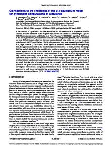
Sym(1) with V1=[10 10] and S1=[2] KnownAtCompileTime(Vector(2): 10 10)

Sym(2) with ?!? KnownAtRuntime(input)

Sym(3) with V3=[U205 U204 U203 ... U108 U107 U106] and S3=[10 10] Reshape(Sym(1), Sym(2))

Figure 5. The IR for reshape([10, 10], input)

trol flow information given by each node, the framework can completely change the order of operations to make execution faster. The LMS framework can lift entire programs, including control flow operations. Using a modified version of the Scala compiler, dubbed scala-virtualized [3], LMS can lift control flow operations such as if clauses and for loops involving wrapped values. A very useful implication is that control flow decisions involving non-wrapped expressions are taken at staging time, while any control flow depending on wrapped values is lifted. In fact, the LMS framework provides nodes, semantics, optimizations and code generation for many common language constructs, such as if clauses, loops, variables, side-effecting operations, etc. They are provided as predefined building blocks that can be imported into the DSL, enabling quick development. So a DSL author only needs to model the domain specific bits of the language and import the common building blocks at no cost. The LMS framework can flatten higher-order constructs. A function passed as a value can be considered a higher-order construct. While Scala allows this and DSL programs certainly make use of it, LMS can force flattening of functions: for example, expecting types Rep[A => B] and Rep[A] => Rep[B] is significantly different: In the first example, passing a function will just get it wrapped, but the second signature will force the passed function to be inlined at the location. StagedSAC uses this because SAC with loops only take expressions, not higher-order functions.

5. StagedSAC Optimizations 4.4

Lightweight Modular Staging

When developing a DSL one may start from scratch by providing a full language compiler or may embed the DSL in a general language, as a library. The main advantage of building a full compiler is the freedom to choose any language syntax and the ability to optimize the generated code. The price to pay is writing a complete implementation of the compiler, from the parser to the code generator. On the contrary, when embedding a DSL the only required effort is to implement the library, but a full program representation is no longer available, so it’s significantly more difficult to optimize code. The Lightweight Modular Staging technique is a middle ground approach, taking the advantages of both compilers and embedding for DSLs. Lightweight staging is based on embedding the DSL while at the same time offering a compiler-like view of the code. Instead of providing concrete library implementations of the DSL primitives, the LMS embedding provides only declarations. From the declarations, the framework builds an IR, that can be further used to optimize the operations and generate the code. LMS scheduling performs generic compiler optimizations with very little effort from the programmer. Once the DSL operation nodes specify their semantics, the LMS framework automatically performs common optimizations such as code motion (moving code outside loops, inside if branches), common subexpression elimination and dead code elimination. These very generic optimizations are enabled by the internal representation of the DSL nodes, as a sea of nodes linked by dependencies. The dependencies can track both data dependencies and effects. Along with con-

This section will present the optimizations added by StagedSAC. StagedSAC features optimizations at several levels: • High-level optimizations: Array Shape Inference, With Loop

Specialization, Input Specialization and Generic Optimizations provided by the LMS framework • Low-level optimizations: JVM-Friendly Code Generation and Loop Tiling 5.1 Array Shape Inference Many optimization transformations rely on shape information. As we have seen before, all with loop optimizations require shape information. Since the language constructs are shape-independent, the IR needs to go through a shape inference stage that determines as much information about the shape as possible. Shape inference requires storing both the shape and the value for each IR node. In SAC shapes are 1-dimensional integer arrays. Operations like reshape and sel use 1-dimensional integer arrays as the shape of their result. In order to infer shapes on such nodes we need to also reason about the values of integer arrays. Inferring the shape of reshape([10, 10], i) as shown in Figure 5, we need to store both the shape and value of the [10, 10] array, as its value becomes the shape of the reshape node. If we did not reason about values, we could only infer that the reshape node has rank two but not its exact shape. While this is a very simple example that could as well be treated as a special case, in the general shape inference algorithm there are many situations that require reasoning about values.

Each IR node introduces constraints on the variables, which are later solved to produce the final shapes. The shape and value inference algorithm is done in three steps: • Gathering the constraints on each node, where each constraint

is an equation between variables • Solving the constraints into variable substitutions • Applying the substitutions to the shape variable of each node to

produce the final shape Constraints are gathered from each of the IR nodes. We can follow the constraint gathering on the example of reshape([10,10], input). The IR is shown in Figure 5. The constraints gathered for the [10, 10] node contain its shape and value, V 1 = [10, 10] and S1 = [2], both of which are known at compile time. There are no constraints generated for input as nothing is known about it. Finally,  the constraints for reshape are: S3 = V 1 and  i S3(i) = i S2(i). The role of the second constraint is to ensure that the transformation corresponds to the same memory block size, as we have seen in Section 2. For all nodes we introduce a generic constraint V x = unknownV alues(Sx). Its role is to fill the value variable with unknown position variables iff the shape is known. It might seem useless, but there is a strong reason to use the unknown position variables in values: after the substitutions such variables retain implicit relations between values. In some cases, by solving unknown values independently the entire shape or value can be discovered. This notion of partially known shapes is our contribution. In the case of SAC, shape information is more coarse-grained (e.g. entire shape available, rank (length of the shape) available and shape unknown). The constraints are solved to substitutions during the unification algorithm. Following our previous example the substitutions generated will be: S3 ⇒ [10, 10] and V 3 ⇒ [U 205 . . . U 106]. Applying the substitutions to the variables yields the exact shapes in Figure 5. Even though this example showcases only shape equality, product equality and unknown values constraints, the full inference algorithm contains 15 types of constraints, such as prefix less than and suffix equals used in sel nodes, length equality, concatenation and others. A constraint may or may not be solvable at a given time. For example the unknown values is not solvable if the exact shape is not known. Once a constraint becomes solvable, it returns a substitution that is applied to all other constraints. This brings more information in existing constraints thus enabling them to be solved. The final list of substitutions is then applied to the shape variable of each node to produce the final solved shape. The unification algorithm is sound but not complete. As we have seen above, not all constraints are solvable immediately. This leads to situations where none or very little information is known about the shapes. Fortunately, the shape inference algorithm is always sound. Any solution that satisfies: • the shape and value equalities (including the unknown position

variable equalities) • the constraints which the unification was not able to solve is a correct typing solution in the context of the program. Despite this, the algorithm is not complete, since not all sets of constraints are solvable all the way to concrete shapes. We keep specific nodes in the IR to infer more information. The generated IR contains high-level operations whereas the final IR for code generation contains only low level operations. The reason is that high-level operations offer stronger constraints on data compared to their low-level equivalents. The low level translation of a + b only mandates shape length equality and less or equal shapes between a and b, while the high level operation a + b mandates stronger and more useful shape equality. After the shape inference

Figure 6. Top-down shape propagation vs Shape inference. The small “RC” nodes are runtime checks to verify shape compatibility. algorithm is run, the high-level operations are transformed into low level with loops that can be specialized and folded. Eliminating redundant checks while generating code. Each IR node generates two sets of constraints: the prerequirements that are necessary for the operation to be successful and the postrequirements that describe the result, once the node has been executed. We separate these two sets of constraints. While generating code, the prerequirements that are not always satisfied are transformed into runtime checks that safeguard the correct operation of the program. Since the postrequirements will always be satisfied by the DSL semantics, there is no need to transform them into runtime checks. The same goes for satisfied prerequirements, which are satisfied by virtue of the postrequirement constraints. The shape inference system in StagedSAC can fill in gaps in the SAC shape system. SAC propagates the shape information topdown, from the input nodes to the output. SAC’s main strength is the function specialization based on input shapes, which could be seen as shape inference with all functions inlined. Using function specialization SAC is able to infer shapes most of the time if the input is given at compile time. However, if the array is read from file along with its rank and shape, SAC will not be able to infer anything about it. On the contrary StagedSAC is likely to infer at least the dimension, if not the complete shape, by propagating shape information upwards, as can be seen in Figure 6. Based on inferred shapes, StagedSAC can generate early tests that triage invalid input. By propagating shape information upstream, StagedSAC constrains the inputs earlier in the execution and moves runtime shape checks outside loops. While runtime checks have a small impact on performance by themselves, they can have a visible impact when iterated in with loops. Figure 6 shows the difference between shape propagation and full inference in terms of runtime checks. In SAC programs, the runtime checks take place late in the execution, but in StagedSAC programs they “bubble up” to the top nodes, making the execution fail faster in case of invalid input. 5.1.1

With Loop Specialization

With Loop Specialization is one of the two with loop optimization currently implemented in StagedSAC. While further optimizations will be implemented with the Delite framework, the current optimization provides significant speedups for big arrays. It works by transforming the generic loop code into a set of nested for loops. This provides a faster execution compared to the backtrack-like code in the case of generic with loops that support any rank. The evaluation section will present the exact numbers to show how with loop specialization speeds up execution. 5.1.2

Input Specialization

The program code is generated and compiled at staging time. In order to gain more information about shapes, the StagedSAC com-

Element Time (ns/matrix element)

case class BinaryOp[A:Manifest:Arith]( inA:Exp[MDArray[A]], inB:Exp[MDArray[A]], op:(A,A)=>A)

500 ns 400 ns 300 ns 200 ns 100 ns 0 ns

extends DeliteOpForEach[A,MDArray[A],A,MDArray[A]] {

0

500

1000

1500

15 ns 10 ns

}

5 ns

Figure 8. Using DeliteOps for data-parallel execution semantics

0 ns 0

500

1000

1500

2000

Matrix Size

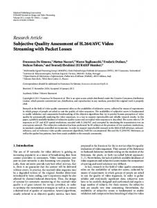
Figure 7. SAC - Total matrix transposition time divided by the total number of elements. Top: Specialization for 1000 × 1000 - 1100 × 1100, none outside. Bottom: Specialization for 2 dimensions, showing cache thrashing starting at 500 × 500 matrices. piler can read program input files ahead of time and extract shape information. While shape information can provide at least rank information in most common cases, for very generic code it may be unable to infer anything. Therefore we can use just in time input specialization to augment shape inference and provide the compiler with the necessary information to optimize the code. If the running time of an algorithm is significant compared to the compile time, just in time input specialization can provide an important speedup. The idea of input specialization is also featured in SAC, but requires a manual annotation in the source code, which is more cumbersome for the developers. The impact of specializing a matrix transposition function in SAC can be seen on the top graph in Figure 7. Input Specialization only extracts shape information from input files. While reading the program input files, StagedSAC could in theory extract the entire program input. The reason we limit input specialization to shapes is that StagedSAC is meant to be an optimizing compiler with partial evaluation and not an interpreter. If all inputs were read at compile time, StagedSAC’s optimizations could theoretically interpret the entire program down to a single value. We want to avoid this, as interpreting the entire program using the slow library code is clearly the worst solution in terms of total execution time. 5.2

Generic Optimizations

After giving LMS the specific semantics of operations, such as nested repetitions in the case of with loops, it can automatically perform generic compiler optimizations: • common subexpression elimination, constant folding, dead-

code elimination • code motion, loop invariant code hoisting (coarse grained, can

change the order of loops) • task parallelism (using the Delite framework, data parallelism

is ongoing work) 5.3

def alloc = new Array[A](prod(shape(inA))) val iter = SpecialOps.internalIterate(shape(inA)) def func = iv => alloc(flatten(iv, shape(inA))) = op(inA(iv), inB(iv))

2000

JVM-Friendly Code Generation

StagedSAC is embedded in the Scala programming language and generates Scala code, which is in turn compiled to JVM bytecode. While programming in Scala is simple and concise, generating efficient code proved to be more challenging. We will highlight two difficulties we faced in the code generation part. JVM arrays are the key to obtaining good speed. Java natively supports base types such as integers, booleans, single and double precision floating point and characters. Arrays containing these base elements are translated to packed arrays in the bytecode,

exactly like in C. But Java also allows creating arrays of any class in the language. Instead of storing the actual object, it creates an arrays of pointers to objects allocated on the heap, adding a level of indirection and affecting memory locality. When targeting the JVM platform, performance-conscious code generators should always use arrays of natively-supported elements. Scala has the same limitation, but provides a more uniform representation on the language-side. This makes it trickier to reason about the memory layout, as arrays of integers may actually be represented using pointers if the array is generic. Object creation destroys locality and adds one more level of indirection. Scala provides support for tuples, so carrying the multidimensional array as a tuple of shape and values would seem like a natural decision. While at first this might seem like a good decision, in fact it’s not. Creating tuples and throwing them away produces redundant calls that can be avoided by creating separate variables for the shape and values. Ranks need not be stored in the structure, as they can be quickly obtained from the length of the shape array. The LMS and Delite code generation is structured as a layered set of code generators, each of which outputs code for a limited set of nodes. This lead to a representation incompatibility between the StagedSAC code generator and LMS built-in generators for if statements, variables and loops. While the StagedSAC code generator expects multidimensional arrays to be unpacked, the LMS generators expect them to be wrapped in tuples. We were able to overcome this problem in the implementation by wrapping arrays in tuples only when they are used outside the StagedSAC code generator. 5.4 Loop Tiling StagedSAC limits the negative effect of irregular, cache-unfriendly access patterns by providing loop tiling. With loops provide data parallel, cache friendly looping in the arrays they create. But the expression passed to the with loop can access data in a cacheunfriendly way, such as in the example of matrix transposition or matrix multiplication. This can severely impact performance. StagedSAC splits the with loop into blocks and iterates over the blocks instead of linearly accessing the data structure. This limits the impact of cache-unfriendly access but incurs a significant overhead for very small arrays. We plan to detect irregular access patterns in the future, so we only add loop tiling where if it is strictly necessary. The effects of exceeding the cache memory for SAC can be seen in the bottom graph in Figure 7.

6. StagedSAC Parallel Execution using the Delite Framework Delite [6, 22] is both a compiler framework and runtime for embedded, parallel DSLs. The Delite compiler framework extends LMS to provide parallel abstractions to DSL authors. These abstractions are Delite ops, and represent common parallel execution patterns such as Map, Reduce, ZipWith, ForkJoin, etc. Figure 8 shows how a simple StagedSAC operation is represented as a Delite op.

By using Delite ops, DSLs also inherit a set of parallel optimizations that Delite provides on top of the generic optimizations provided by LMS. The most important of these is fusing; all Delite ops are represented internally as loop-based operations of a fixed size, and multiple loops are fused into a single loop when possible (i.e. when there are no unsatisfiable dependencies across the loops). Fusion helps eliminate unnecessary allocations for temporary arrays, which is crucial to obtaining high performance in a language with immutable semantics such as SAC. Furthermore, Delite handles code generation for all Delite ops, and translates Delite ops to efficient parallel implementations for both CMPs and GPUs. This translation is possible because the semantics of Delite ops represent well known execution patterns; the optimized implementation of these patterns for each device is handled once and for all by the Delite framework and runtime, and all Delite DSLs can leverage them. Every op in a Delite DSL is emitted as a kernel for multiple platforms. Not all operations can be generated for every platform (e.g. operations with dynamic memory allocation are usually not well suited for GPUs), but the code generation is successful if the op can be generated for at least one platform. Any operation in the application that is not a Delite op is implicitly wrapped as a DeliteOpSingleTask, or a sequential operation that will be generated as a Scala kernel. Besides the kernels for each platform, Delite also generates an execution graph that captures data and control dependencies between kernels. The execution graph and generated kernels form the inputs to the Delite runtime. The Delite runtime maps the execution graph and kernels to parallel, heterogeneous hardware. Based on the resources available (e.g. number of processor cores and GPUs), Delite determines which device to run an op on and when to schedule it. Delite transparently handles difficult issues such as communication (even across address spaces, e.g. to a GPU) and synchronization across ops. These are tasks that any embedded DSL or stand alone DSL would traditionally have to implement individually to achieve parallel performance, despite their commonality across DSLs. StagedSAC’s operations naturally mapped to the existing set of Delite ops (although required extending Delite to support strided access patterns). Any embedded DSL that is targeted at Delite that can match their domain operations to existing Delite ops can easily take advantage of heterogeneous parallelism, as we have shown. The situation is more complicated, though not hopeless, if a new kind of parallel pattern is needed. Delite is designed to be extensible, but adding new Delite ops still requires knowledge of how Delite works. In the future, we plan to make this process even more modular. Furthermore, we believe that the set of Delite ops correspond to a ”parallel instruction set”, and that as more Delite ops are added to cover a broader set of DSLs, the coverage of this instruction set will continue to increase while the corresponding incremental cost of building a new DSL on top of Delite will decrease.

7. Evaluation As stated in the contributions, the evaluation contains three parts: • the evaluation of the time required to develop StagedSAC • the development of SAC in terms of performance and compar-

isons to SAC • the preliminary results on generating parallel code using the

Delite framework 7.1

Development Time

The StagedSAC was developed by the first author, without previous knowledge of Scala, LMS and Delite. It was developed during two semester projects. We can split StagedSAC’s evolution into three phases:

• From scratch to the LibrarySAC implementation, which took

approximately 2 months, including learning Scala and SAC • From LibrarySAC to the first StagedSAC prototype, which took

approximately 2 months, including learning how to use the first versions of the LMS framework • From the first StagedSAC prototype to the current StagedSAC compiler, which took approximately 3 months, including learning Delite The same three phases are benchmarked in the performance evaluation. Each stage of the evolution reduced the running time for the benchmarks by an order of magnitude. 7.2 Testing Setup For testing we used a Core 2 Duo machine running at 2GHz. The processor had 32K data + 32K instructions level 1 cache and 2048K level 2 cache. The RAM memory limit was set at 2GB. For all the tests the input was loaded into memory before the algorithm execution and stored back into memory, therefore the hard-drive was not involved in the benchmark. StagedSAC generates Java bytecode, therefore special benchmarking had to be done to ensure stable results. The Java Virtual Machine performs Just-In-Time compilation of the bytecode and optimizes the code on the fly. For the benchmarks we ran the code several times in the same Java Virtual Machine in order for the code to be fully compiled and optimized. Indeed, the first 2 or 3 runs of the same algorithm provided very long running times. We also noticed that after 5 runs, the time stabilized and we could measure an almost-constant value. Another problem we faced was garbage collection: since the memory management is done automatically when running out of heap space, we wanted to avoid this affecting the results. Therefore between any two runs we ran the garbage collector. 7.3 Benchmarks The evaluation was performed on two different algorithms: The game of Life simulation and the PDE1 benchmark. We will present the two benchmarks in detail and present the results. The “game of life” benchmark is a simulation of cells dying and being born, with discrete generations. The benchmark has been implemented in both SAC (Figure 2), LibrarySAC (Figure 3) and StagedSAC (Figure 4). We ran 1000 iterations of a 10 × 10 simulation board and measured execution time. The PDE1 benchmark represents a three dimensional approximation of Poisson equations. It was presented in the SAC journal paper [24]. We use this benchmark since it was also used in HPF and the SAC paper. From all implementations of the PDE1 benchmark we picked the lowest running times, since a real world programmer would use the fastest implementation available. We tested PDE1 on 64 × 64 × 64 arrays. PDE1-64 Game of Life-10 1 iteration 1000 iterations LibrarySAC 3123ms 417357ms StagedSAC - Prototype 1932ms 2672ms StagedSAC - Current version 379ms 323ms SAC Compiler 22ms 99ms The evolution from LibrarySAC to the StagedSAC prototype roughly corresponds to the set of high-level optimizations. These include the generic optimizations provided by the LMS framework, the simple with loop specialization using the shape inference algorithm we presented. These provided an initial speedup that showed with the little effort of embedding the compiler it was possible to obtain a significant speedup. StagedSAC’s evolution form prototype to the current version roughly corresponds to the set of low-level optimizations. They impact the code generation and are intended to be aware of the Benchmark

60

50 Total Transposition Time (s)

[3] The Scala-virtualized fork of the Scala compiler. URL https: //github.com/TiarkRompf/scala-virtualized. [4] StagedSAC repository, built as a DSL insde Delite. URL https: //github.com/stanford-ppl/Delite/tree/mdarrays.

Generic Shapes (*) Input Specialization, no Loop Tiling Input Specialization, Loop Tiling

40

30

20

10

0 0

2000

4000

6000 Matrix Size

8000

10000

12000

Figure 9. Automatic input specialization using JIT-compilation in StagedSAC, running matrix transpose platform they are running on. The only new high-level optimization is input specialization, which was meant to complement shape inference for the cases where the code was very generic. The effect of the loop tiling can be seen in Figure 9. If the index vector’s rank is known at compile time, the with loop can be specialized. The total time to transpose a square matrix n × n is shown as a function of the matrix size n. The 3 lines, in the order highest (longest time) to lowest, represent: • StagedSAC matrix transposition without shape knowledge, using the most generic algorithm • StagedSAC matrix transposition, with input specialization without loop tiling • StagedSAC matrix transposition, with input specialization and loop tiling While it is clear that StagedSAC is not as fast as the SAC compiler, each new optimization brings performance improvements at a fraction of the cost of implementing it in SAC. 7.4

Parallel Execution

For now, we have a very coarse-grained parallel model and the overhead is comparable to the gains for most of the programs. However, if the program executes parallel operations of almost-equal size, a speedup can be observed (in the Game Of Life benchmark). For 2 cores we obtained a speedup of 1.65×. We expect to obtain almost linear speedups when using data parallel DeliteOps and loop fusion and folding. PDE1-64 Game of Life-300 Benchmark 10 iterations 10 iterations StagedSAC - 1CPU 3918ms 3841ms StagedSAC - 2CPU 3906ms 2326ms

8. Conclusions We presented our experiences with StagedSAC, a DSL developed to mimic the functionality of the multidimensional array language SAC. We showed how Lightweight Modular Staging significantly reduced the effort necessary to develop the StagedSAC compiler. We showed it is possible to augment the LMS-based compiler with complex analysis phases such as shape inference and optimized code generation.

References [1] The Delite framework repository. URL https://github.com/ stanford-ppl/Delite. [2] The Lightweight Modular Staging framework repository. URL https://github.com/TiarkRompf/ virtualization-lms-core.

[5] T. Brandes and F. Zimmermann. ADAPTOR - A transformation tool for HPF programs. Birkhuser Basel, 1994. ISBN 3764350903. [6] K. Brown, A. K. Sujeeth, H. Lee, T. Rompf, H. Chafi, M. Odersky, and K. Olukotun. A heterogeneous parallel framework for domain-specific languages. PACT, 2011. [7] H. Chafi, Z. DeVito, A. Moors, T. Rompf, A. K. Sujeeth, P. Hanrahan, M. Odersky, and K. Olukotun. Language virtualization for heterogeneous parallel computing. OOPSLA, 2010. [8] P. Charles, C. Grothoff, V. Saraswat, C. Donawa, A. Kielstra, K. Ebcioglu, C. von Praun, and V. Sarkar. X10: an object-oriented approach to non-uniform cluster computing. OOPSLA, 2005. [9] C. Consel and O. Danvy. Tutorial notes on partial evaluation. In Proceedings of the 20th ACM SIGPLAN-SIGACT symposium on Principles of programming languages, POPL, 1993. [10] C. Consel and S. C. Khoo. Parameterized partial evaluation. ACM Trans. Program. Lang. Syst., 15:463–493, July 1993. [11] L. Damas and R. Milner. Principal type-schemes for functional programs. In Proceedings of the 9th ACM SIGPLAN-SIGACT symposium on Principles of programming languages, POPL, 1982. [12] G. Dubochet. Embedded Domain-Specific Languages using Libraries and Dynamic Metaprogramming. PhD thesis, EPFL, 2011. [13] Y. Futamura. Partial evaluation of computation processan approach to a compiler-compiler. Higher-Order and Symbolic Computation, 12: 381–391, 1999. [14] C. Grelck, S.-B. Scholz, and K. Trojahner. With-Loop Scalarization Merging Nested Array Operations. IFL. 2005. [15] C. Grelck, K. HinckfuB, and S.-B. Scholz. With-Loop Fusion for Data Locality and Parallelism. IFL. 2006. [16] K. E. Iverson. A Programming Language. AIEE-IRE ’62 (Spring), pages 345–351, New York, NY, USA, 1962. ACM. [17] C. B. Jay. The FISh language definition. Technical report, 1998. [18] S. Kuthe. A Hybrid Shared Memory Exection Model for SAC. Diploma thesis, Institute for Software Technology and Programming Languages, University of Lubeck, 2005. [19] J. McGraw, S. Skedzielewski, S. Allan, D. Grit, R. Oldehoeft, J. Glauert, I. Dobes, and P. Hohensee. SISAL: Streams and iteration in a single assignment language: Reference manual. Technical Report LLL/M-146, Lawrence Livermore National Laboratory, 1983. [20] M. Odersky, L. Spoon, and B. Venners. Programming in Scala: A Comprehensive Step-by-Step Guide, 2nd Edition. Artima Inc, 2011. ISBN 0981531644. [21] T. Rompf and M. Odersky. Lightweight modular staging: a pragmatic approach to runtime code generation and compiled DSLs. GPCE ’10. [22] T. Rompf, A. K. Sujeeth, H. Lee, K. J. Brown, H. Chafi, M. Odersky, and K. Olukotun. Building-Blocks for Performance Oriented DSLs. PACT, 2011. [23] S.-B. Scholz. With-loop-folding in Sac-condensing consecutive array operations. IFL. 1998. [24] S.-B. Scholz. Single Assignment C: efficient support for high-level array operations in a functional setting. J. Funct. Program., 13: 1005–1059, November 2003. [25] S.-B. Scholz, S. Herhut, F. Penczek, and C. Grelck. SAC 1.0 Tutorial, 2010. URL http://www.sac-home.org/publications/ tutorial.pdf. [26] A. K. Sujeeth, H. Lee, K. J. Brown, T. Rompf, H. Chafi, M. Wu, A. R. Atreya, M. Odersky, and K. Olukotun. OptiML: An Implicitly Parallel Domain-Specific Language for Machine Learning. In ICML’11, 2011. [27] K. Trojahner and C. Grelck. Dependently Typed Array Programs Don’t Go Wrong. Journal of Logic and Algebraic Programming 78(7), 2009.