A Case Study: Validation of Guidance Control Software Requirements for Completeness, Consistency and Fault Tolerance Frederick T. Sheldon, Hye Yeon Kim, and Zhihe Zhou Washington State University Pullman, Washington 99164-2752, USA
[email protected] |
[email protected] |
[email protected] principally provides control during the terminal phase of descent for the Viking Mars Lander. The lander has three accelerometers, one Doppler radar with four beams, one altimeter radar, two temperature sensors, three gyroscopes, three pairs of roll engines, three axial trust engines, one parachute release actuator, and a touch down sensor. After initialization, the GCS starts sensing the vehicle altitude. When a predefined engine ignition altitude is sensed, the GCS begins guidance and control of the vehicle. The purpose of this software is to maintain the vehicle along a predetermined velocityaltitude contour. Descent continues along this contour until a predefined engine shut off altitude is reached or touchdown is sensed. The ARSP (Altimeter Radar Sensor Processing) is a sub-module of the GCS. This functional unit reads the altimeter counter provided by the altimeter radar sensor and converts the data into a measure of distance to the surface of Mars. If uncovered failures occur, the lander could fail to land on the surface even though it had successfully traveled the long distance from Earth to Mars. Therefore, assessing the SRS for the reliability and performability is required for the mission critical software [3, 4].
Abstract In this paper, we discuss a case study performed for validating a Natural Language (NL) based software requirements specification (SRS) in terms of completeness, consistency, and fault-tolerance. A partial verification of the Guidance and Control Software (GCS) Specification is provided as a result of analysis using three modeling formalisms. Zed was applied first to detect and remove ambiguity from the GCS partial SRS. Next, Statecharts and Activity-charts were constructed to visualize the Zed description and make it executable. The executable model was used for the specification testing and faults injection to probe how the system would perform under normal and abnormal conditions. Finally, a Stochastic Activity Networks (SANs) model was built to analyze how fault coverage impacts the overall performability of the system. In this way, the integrity of the SRS was assessed. We discuss the significance of this approach and propose approaches for improving performability/fault tolerance.
1.
Introduction
1.1.
High assurance systems demand rigorously engineered software. A failure in the control software of mission critical systems can be disastrous. It is difficult to create a reliable requirements specification because such control software tends to be highly complex. Moreover, it is well known that the majority of software errors are introduced during the requirements phase [1, 2]. To avoid problems in the latter development phases and reduce life-cycle costs, it is crucial to ensure that the specification be reliable. By reliable, we mean: (1) is the specification correct, complete, and consistent? (2) Can the specification be trusted to the extent that design and implementation can commence while minimizing the risk of costly errors? (3) How can we analyze the specification to prevent the propagation of errors into the downstream activities? The Guidance and Control Software (GCS)
Related Works
There have been numerous studies conducted that combine a Zed representation with some formal method or design notation. A hybrid formal method, called PZnets that combine Petri nets and Zed notations, was developed [5]. The benefits provide a unified formal model for specifying the overall system structure, control flow, data types and functionality. Sequential, concurrent and distributed systems are modeled using a valuable set of complementary compositional analysis techniques. This approach has been successfully applied to model some known high assurance and concurrent systems. However, the lack of modular and hierarchical facilities precludes this approach to be applied to large systems. Bussow and Weber present a mixed method consisting of Zed notations and Statecharts [6]. Each method was applied to a separate part of the system. Zed
1
Networks (SANs) were used to assess the dependability of the software in terms of fault detection and coverage since it is well suited for performability and dependability modeling.
was used in defining the data structures and transformations. Statecharts were used in representing the overall system and showing the reactive behavior. The Zed notations were type checked with the ESZ type checker but the Statechart semantics were not fully formalized. In addition, we reviewed several other case studies that utilized Zed for concretely defining data while using Statecharts as a behavioral description and evaluation method [7-9]. Hierons, Sadeghipour, and Singh present a hybrid specification language µSZ[10]. The language uses Statecharts to describe the dynamical system behavior and Zed to describe the data and data transformations. Their data abstraction technique uses information derived from the Zed specifications to produce an extended finite state machine (EFSM) defined by the Statecharts. The EFSM poses properties that can be utilized during test generation. These properties help solve the problems of setting up the initial state and checking the final state of a test to assist in test automation. Both the dynamic behavior specified in Statecharts and the individual operations are checked using this method. Dugan and Trivedi present several different models for predicting coverage in a fault tolerant system to illustrate their methods for accurately predicting and assessing dependability [11]. They classified three error categories: permanent, intermittent, and transient. Models used in their study were Markov, semi-Markov, non-homogeneous Markov, and extended stochastic Petri Nets. They investigated the sensitivity of the system reliability to the coverage parameter and the sensitivity of the coverage parameter to various error handing strategies. Sanders and Malhis showed the applicability of SAN in dependability evaluation [12]. State space explosion is a common problem when using Markov models directly for analyzing a realistic design. SANs, together with reduced base model construction techniques, can result in tractable Markov models for many parallel and distributed systems. In our study, Zed was used to clarify ambiguous statements found in the SRS. Zed was chosen because it provides a concrete way to transform requirements into state-based models using the schematic structuring facilities. The transformation elucidates assumptions and provides mechanisms for refining abstract specifications into concrete ones for clarifying data and functional definitions. Statecharts were chosen to model the Zed specifications because a key goal was testability and predevelopment evaluation. A clear distinction of our approach with other approaches is that we did not combine Zed and Statecharts together. We translated the SRS into Zed completely and then translated the Zed specification into Statecharts. Stochastic Activity
1.2.
Completeness and Consistency
The completeness of a specification is defined as the lack of ambiguity from the implementation perspective. The specification is incomplete if the system behavior is not specified precisely because the required behavior for some events or conditions is omitted or is subject to more than one interpretation [13]. Consistency means that the specification is free from conflicting requirements and undesired nondeterminism [14]. 1.3.
Fault Tolerance
Traditionally, fault-tolerance has referred to building systems from redundant parallel components [15]. A fault-tolerant system is a system that has the ability to respond to unexpected hardware or software failures. Components in a system interact with each other as well as the environment. There are many levels of faults may occur in any component. The undesired operation inside the component, an error propagated from another component, or user error (mistake) can cause faults. Theoretically, no system is absolutely fault free. There are plenty of catastrophic failures to substantiate this [16]. The probability of system failure decreases in accordance with a cautious specification and design process. However, the more complex the system, the more difficult it is to achieve high performance and fault tolerance. Software is considered as fault-tolerant (robust) if and only if the software: (1) is able to compute an acceptable result even if the program itself suffers from incorrect logic; and (2) whether correct or incorrect, is able to compute an acceptable result even if the software itself receives corrupted incoming data during execution. The key to this definition is to determine what is "acceptable." For the ARSP module of the GCS, the “acceptable” result means the distance from the vehicle to the surface of Mars, computed by the ARSP, should be accurate enough to result in a successful landing. If there are deviations, these errors should not cause false actions in other modules that may lead to catastrophic or incorrect operation. 1.4.
Informal and Formal Specifications
The typical SRS highly depends on natural language. Natural language based specifications are often subject to multiple interpretations. Even when such specifications are developed systematically, it is
2
Statecharts consist of where S is a set of states, T is a set of transitions, E is a set of events and V is a set of variables. States are either BASIC, OR, or AND states where BASIC states have no sub-states while OR states do have sub-states that are related to each other by an exclusive-or relation. Being in an OR state means being in only one of its sub-states. AND states have sub-states, called orthogonal components, that are related by an and relation. Being in an AND state implies that being in all of its orthogonal components. Changes among states are represented by a transition (i.e., event [condition] / action). An event is an instantaneous occurrence of a stimulus (trigger), a condition is a predicate that must be satisfied for a transition to occur and an action may generate other events or perform computations. Thus, Statecharts = finite state machines + depth + orthogonality + broadcast. The depth is achieved by OR states and orthogonality is achieved by AND states. Broadcast is used to communicate among states and is achieved by the action of a transition. In other words, when a transition is triggered, an action generates an event and this event is assumed to be globally broadcast [19]. Statecharts (STATEMATE Magnum, a product of iLogix, was used for this case study.) provide a natural way to specify complex reactive systems both in terms of how objects communicate and collaborate and how they carry out their own internal behavior. Together Activitycharts and Statecharts are used to describe the system functional building blocks, activities and the data that flows between them. These languages are highly diagrammatic in nature, constituting full-fledged visual formalisms, complete with rigorous semantics providing an intuitive and concrete representation for inspecting and checking for conflicts [20]. These two formalisms, Activity-charts and Statecharts, were used to specify our conceptual system model for symbolic simulation. In this way, we verified our assumptions, injected faults, and identified hidden errors constituting inconsistencies or incompleteness in the specification.
difficult to ensure their integrity without some form of correctness checking. Generally, correctness checking obligates the use of a mathematically based requirements specification language (RSL). Such languages are notoriously difficult to understand, and minimally require a proficient level of knowledge in discrete mathematics and/or some formal logic system. This poses a serious concern to industry because many different classes of requirements exist. Different stakeholders typically represent various ways of looking at the problem. Thus, a multi-perspective analysis is important, as there is no single correct way to analyze system requirements [17]. The usefulness of the requirements specification is diminished by not being understandable to the diverse set of stakeholders. Nevertheless, to avoid the confusion caused by ambiguity, the merits of two different mathematically based RSLs were investigated.
2.
Methods
The sequence of the methods application is as follows. First, the NL-based GCS specification was transformed using the Zed notation. Zed Schemas were abstracted from GCS components. This compositional process helped to clarify ambiguities. Second, the Schemas were transformed into Statecharts/Activitycharts and symbolically executed to assess the model’s behavior using the GCS-specified mission profile. Finally, a SAN model was developed to analyze the fault tolerance of the system. In this section, we provide brief descriptions of each method that were used in this study. 2.1.
Zed
The Zed notation is a mathematical language with a theory of refinement between abstract data types. In combination with natural language, it can be used to produce a formal specification. We may reason about this specification using the proof techniques of mathematical logic. We may also refine the specification, yielding another description that is closer to executable code [18]. Schema's are the main structuring mechanism used to create patterns and objects. The notation is used to model systems in terms of state. We describe the state of the system and explain the relationship between ARSP and the state of various components. The production of such a specification helps us to understand requirements, clarify intentions, and construct proofs (i.e., identify assumptions and explain correctness). These facilities provided by Zed were useful and essential in clarifying ambiguities and solidifying our understanding of the requirements. 2.2.
2.3.
SANs
Stochastic Activity Networks is an extension of the Generalized Stochastic Petri Net. In addition to transitions (called activities) and places, SANs use two new types of components: Input gates and Output gates[21]. Input gates are used to connect places with activities. Each input gate is associated with a predicate and a function. In order to enable the activity, all predicates of its input gates must be true and all places, immediately connected to it, must contain at least one token. The function of the input gate specifies how to change the tokens of the places that connect to this input gate. Output gates are associated with functions. Like
Statecharts
3
Figure 1 provides an example, using the FRAME_COUNTER input variable that illustrates the complete translation from Zed to Statecharts. The FRAME_COUNTER is defined as an integer with range
input gate functions, output gate functions also specify how many tokens are removed from or added to the places that are connected to the output gate. When an instantaneous activity is enabled, it can fire immediately. If it is a timed activity, it can fire after a time delay determined by the assigned probability distribution. The firing of an activity results in: (1) all input gate functions are executed, (2) each immediatelyconnected input place has one token removed, (3) all output gate functions are executed, and 4) each directlyconnected output place has its token incremented.
3.
Transformation Specifications
of
the
[1, 2 31 − 1 ]. In Zed, the FRAME_COUNTER is declared as a set of natural numbers in the signature part and the range of the variable is defined in the predicate part (lower half of the schema). The Statechart representation of the FRAME_COUNTER variable is presented with the direction of data transfer from EXTERNAL into the ARSP Module (see Figure 1 for the details). Its type and value range are defined in the Statemate data dictionary. In translating from the NL-based SRS to Zed, four ambiguously specified requirements were identified. The first one concerns the rotational direction assumed by the use of the term “rotate.” Secondly, an undefined third order polynomial was revealed that is used to estimate the AR_ALTITUDE value [22]. The third issue (i.e., ambiguity) concerns the use of the AR_COUNTER variable for two different purposes, which imply that it has two different types. Finally, there is uncertainty regarding the scope of the AR_COUNTER variable that brings into question which module should use and/or modify this variable. Given these various issues, two scenarios were considered. The first scenario assumes the AR_COUNTER is updated within the ARSP module while the second scenario does not. Both scenarios were constructed separately and compared to understand how Zed could be useful in clarifying ambiguity and avoiding conflicts. Scenario one supposes that the separate constraints (i.e., one variable with different types) defined in the SRS should be represented by separate variables (i.e., Echo and AR_COUNTER). In the SRS, the sign bit of AR_COUNTER represents whether the radar echo pulse is received on time. In scenario one, this condition is split off into the Echo variable while in scenario two the Echo variable is not introduced. The Zed specification is considered consistent with the SRS as long as the newly defined Echo variable does not cause a side affect outside of the ARSP module (i.e., if by chance, some other function/module accesses the sign bit). Because we have chosen in scenario one to introduce a new ARSP input variable we must decide where and how this variable is updated. Accordingly, we modified the Zed version of the ARSP specification to account for two separate variables. As a result of iterative refinements of the Zed specification, we found that the Echo variable must be treated as an additional ARSP input because there is no other way to determine if the radar echo pulse has been received. This in turn caused the whole specification to be revised to reflect the principle that mandates decoupling data [17]. Therefore,
Different
We now discuss the transformation from the SRS to the Statecharts representations via Zed. The Altitude Radar Sensor Processing (ARSP) module specification showing inputs, outputs, and subsystem processing descriptions was chosen for the purpose of our study. Module Specification
NL-Based SRS
Data Dictionary
NAME: FRAME_COUNTER DESCRIPTION: Counter containing the number of the AR_COUNTER present frame AR_STATUS USED IN: AECLP, ARSP, CP, GP, TDLRSP K_ALT UNITS: none OUTPUT 31 RANGE: [1, 2 -1] AR_ALTITUDE AR_STATUS DATA TYPE: Integer*4 K_ALT ATTRIBUTE: data DATA STORE LOCATION: EXTERNAL PROCESS: It is only necessary that this functional module ACCURACY: N/A INPUT AR_ALTITUDE AR_FREQUENCY FRAME_COUNTER
Zed Specification
ARSP_RESOURCE
1 FRAME_COUNTER? : N 2 AR_ FREQUENCY? : R 3 AR_COUNTER? : Z 4 K_ALT_1, K_ALT_2, K_ALT_3, K_ALT_4, K_ALT_NEW: {0,1} 5 AR_ALTITUDE_1, AR_ALTITUDE_2, AR_ALTITUDE_3, AR_ALTITUDE_4, AR_ALTITUDE_NEW: R 6 AR_STATUS_1, AR_STATUS_2, AR_STATUS_3, AR_STATUS_4, AR_STATUS_NEW: {healthy, failed} 7 K_ALT: K_ALT_1 x K_ALT_2 x K_ALT_3 x K_ALT_4 8 AR_STATUS: AR_STATUS_1 x AR_STATUS_2 x AR_STATUS_3 x AR_STATUS_4 9 AR_ALTITUDE: AR_ALTITUDE_1 x AR_ALTITUDE_2 x AR_ALTITUDE_3 x AR_ALTITUDE_4 AR_COUNTER? e -1..32767 AR_FREQUENCY? e 1..2450000000 FRAME_COUNTER? e 1..2147483647 AR_ALTITUDE_1 e 1..2000 ¶ AR_ALTITUDE_2 e 1..2000 ¶ AR_ALTITUDE_3 e 1..2000 ¶ AR_ALTITUDE_4 e 1..2000 ¶ AR_ALTITUDE_NEW e 1..2000
Statecharts ARSP RUN_PARAMETER
AR_FREQUENCY
AR_ALTITUDE
@INIT
AR_ALTITUDE
CALCULATE
AR_STATUS
SENSOR_OUTPUT
K_ALT AR_COUNTER
GUIDANCE_STATE
@ALTIMETER AR_STATUS
EXTERNAL FRAME_COUNTER
K_ALT
Figure 1 Mapping example from NL-based to Statecharts
The SRS provides a data dictionary with variable definitions, type, units, and a brief description of variables and functions. This descriptive information is shown in [22]. We abstracted the NL-based module specification into Zed preserving variable names, operations (i.e., functionality), dependency and scope.
4
the interpretation of scenario one is inconsistent with the SRS. On the other hand, in scenario two no additional variables were defined. Only those variables defined in the SRS were specified and all the requirements specified in ARSP were covered. Therefore, this reformulation of the SRS was considered as a complete and consistent transformation. We chose scenario two for this reason as the basis from which to build the Statecharts. In this way, Statemate could be used to analyze a model that properly conformed to its requirements which we believed would be useful in feeding back the results of our assessment (i.e., symbolic simulation). We also wanted to confirm what we had seen using Zed using this other type of formalism namely Statecharts and determined if indeed our reformulation revealed similar ambiguity. The details of the Zed specification for scenario two are described in [22].
4.
The Transformation Statecharts
from
Zed
RUN_PARAMETERS
TDLRSP .3
GUIDANCE_STATE
GSP .4
TSP .5
TDSP .6
SENSOR_OUTPUT
The ARSP Activity-chart shows the data flow between the data stores and the ARSP module based on the information (albeit it does not show which parameters go where.) The direction of the data flow is given by Figure 3, which follows from the information contained in the SRS data dictionary [23].
5.
to
Integrating Fault Tolerance to the ARSP Specification
The GCS software runs in a harsh environment and depends on correct operation of the hardware. Cosmic radiation could cause memory bits to flip, and hardware sensors might fail. These hardware failures are beyond the level that GCS software can control, although the GCS must detect such failures; the actual masking counter measure would typically be accomplished through redundancy (i.e., using error correction memory or shielding the memory from radiation, and providing backup sensors in case of sensor failure). As shown in Figure 3, the ARSP is a component of the sensor processing logic and consequently a component of the entire GCS software system. Sensor data are fed into the ARSP to produce a measure of distance from the vehicle to the surface of Mars. The value of altitude is the output of ARSP and is further used by other components to guide the terminal decent of the vehicle. As long as the output is correct, the ARSP does not introduce errors to the system. There are two possible sources of error. One is an input error, which would cause an incorrect output. The other case would involve some logical ARSP design flaw. This type of error would cause correct input data to produce incorrect output. The goal of fault tolerance in the ARSP is to detect and cover these errors so that no error will propagate to other system components. A robust specification should specify how to cope with errors. It is not only important to specify a correct algorithm but also how to handle errors or exceptions. An internal error is truly an unexpected error. It not only depends on a carefully designed specification but also on its correct implementation. In order to detect and cover an internal error, the specification can require different implementations running in parallel. The outputs of all running implementations are checked. If there are differences between them, there might be an
INI CURRENT_STATE
KEEP_PREVIOUS_VALUE>
ASP .1
Figure 3 DFD 2.1 SP - Sensor Processing [23]
An ARSP project was created within the Statemate framework. Graphic editors were used to create Statecharts and Activity-charts. Once the graphical forms were characterized, state transition conditions and data items were defined.
[MOD(FRAME_COUNTER, 2)=0]/ AR_ALTITUDE(3):=AR_ALTITUDE(2); AR_ALTITUDE(2):=AR_ALTITUDE(1); AR_ALTITUDE(1):=AR_ALTITUDE(0); AR_STATUS(3):=AR_STATUS(2); AR_STATUS(2):=AR_STATUS(1); AR_STATUS(1):=AR_STATUS(0); K_ALT(3):=K_ALT(2); K_ALT(2):=K_ALT(1); K_ALT(1):=K_ALT(0)
ARSP .2
EXTERNAL
[MOD(FRAME_COUNTER, 2)=1]/ st!(CALCULATE)
CALCULATION
Figure 2 ARSP INI Statechart
These items and/or conditions trigger activities and state transitions that occur within the Statemate model based on definitions within the “data dictionary” and/or the “data bank browser.” The Activity-chart (Statechart part of Figure 1) and Statecharts (shown in Figure 2, also refer the [22]) reflect all variables/conditions defined in our Zed formulation. During simulation, various color changes help to show the sequence of state changes that occur to validate the system according to its specified structure (based on our Schema signatures) and constraints (based on our Schema predicates). We changed initial (and current) values and conditions while at the same time rerunning and/or resuming the simulation in the process of verifying our assumptions against the Statechart specification. In this way, we exercised the Statechart-based model and generated C code directly from the charts.
5
found some week points of the system where faults were lurking; (4) Consequently, there are many designs decisions to be made in the process of developing a model (i.e., specification). Finding the correct formulation is a process of refinement and validation, which was facilitated using formal specification and symbolic simulation. Some requirements were found to be inconsistent/incomplete because they produced incorrect results. Based on the simulation results using fault injection we discovered that the SRS was incomplete. To remedy the situation we suggest that the AR_FREQUENCY value be bounded to prevent the AR_ALTITUDE value from exceeding its limit either one of the following condition should be included: 1¯AR_FREQUENCY¯AR_COUNTER * 75000, or AR_COUNTER = -1 v (0 ¯ AR_COUNTER ¯ AR_FREQUENCY/75000). Without either one of the restrictions, the AR_ALTITUDE output value exceeds its limit.
internal error. We can further decide which one has an error and use the correct output. We can also force the faulty one to shut down or restart.
6.
Specification Testing
Now we discuss the results of our validation effort based on symbolic simulation of the ARSP Statechart model. In effect, we verified that the ARSP subunit requirements are complete and consistent by running the simulation against all of the Activity/Statecharts. The data used in the simulation is provided in Table 1. Table 1 ARSP Specification Test Cases
Variable FRAME_COUNTER AR_STATUS AR_COUNTER
Case 1 2 DC -1
Case 2 2 DC 19900
Case 3 1 [0, 0, 0, 0] -1
Case 4 1 DC 20000
Case 5 3 [0, 1, 0, 0] -1
X Event occured, DC Don’t Care.
Table 2 ARSP Outputs from the Simulation
Variable AR_STATUS K_ALT AR_ALTITUDE
Case 1 KP KP KP
Case 2 KP KP KP
Case 3 Case 4 Case 5 [1, 0, 0, 0] [0, -, -, -] [1, 0, 1, 0] [1, 1, 1, 1] [1, -, -, -] [0, 1, -, 1] [*, -, -, -] [2000,-,-,-] KP
- Don’t care, KP Keep Previous value,
7.
* An estimated value.
Five conditions (Case 1-5) as shown in Table 1 were defined to test the charts we developed. They represent the way we visualized and were able to scrutinize the Zed specification. The AR_FREQUENCY value was fixed at 1,500,000,000 to calculate the value of AR_ALTITUDE for all test cases. In the material presented below, we’ll explain how each of the conditions was evaluated which should help to convince the reader that the ARSP subunit is significantly complex (one of six different sensor units used by the GCS). The values of the ARSP output variables are given in Table 2 (KP in indicates that the first two element values of the output are same). All the output values are the same as expected. All the transitions, activities, and states in the charts were activated precisely as expected. All of the variables were updated as expected. The expected values were calculated based on the given equations in NL-base SRS. Therefore, the result of this simulation show the previous Zed specification was developed correctly. We used simulation of the specification for discovering hidden faults and their location. To accomplish this, faults were injected into the model to simulate a memory corruption (expected due to the harsh space born lander mission environment.) Four new issues arose during the fault injection process. (1) Some correct inputs produced incorrect outputs; (2) The Statecharts approach has a better chance of predicting possible faults in the system. (Because the Zed spec cannot provide a way of predicting the transitions from state to state [Zed is not executable]); (3) During the symbolic simulation, we
The Fault Coverage Analysis
Figure 4 gives an abstract SAN model of the ARSP. There are only a few details about how the ARSP computes the output. Instead, we use the SANs to model fault coverage to evaluate the dependability of the entire system[12]. The ARSP module can work in either of two modes: normal or diagnostic mode. In normal mode, the ARSP completes useful works. While in diagnostic mode, it concentrates on detecting and covering errors. Therefore, the ability to find and cover an error is stronger in diagnostic mode than in normal mode. The current working mode of the system is represented by a token in either the place normal or the place diag. Activity n2d represents the switching from normal working mode to diagnostic mode, while d2n for switching back to normal mode. Initially, the system is in normal mode, represented by a token in normal. If there is an input, represented by a token in place in, this input data could be incorrect with probability pInputErr, or correct with probability (1- pInputErr). If the input data were incorrect, a token would be put in the place error. If the input data are correct, the internal error might cause an error to occur, and then a token would be put in the place error. An error in the system is represented by the token in the place error. If there is an error, the system will try to detect and cover it. This system’s ability to cover an error depends on the system mode. If the system failed to cover the error, a token would be put in the place out_wrong, which means that the system produced an erroneous output. If no error occurs or the error is covered, a token will be put in the place out_right.
6
detected, the output error probability is much lower (less than 0.08), given the same input error. Probability of Output Error
Output Error vs Working mode 0.1
pInputErr = 0.00 pInputErr = 0.10 pInputErr = 0.20
0.08 0.06 0.04 0.02 0.1
Figure 4 SAN model of ARSP
0.15
0.2
0.25
0.3 0.35 in_diag
0.4
0.45
0.5
Figure 5 Error Probability in different working mode
Probability of Output Error
We used the Accumulated Reward Solver of UltraSAN for two cases of analysis. We are interested in how the various parameters will affect the probability of output an error. In other words, what is the error probability of ARSP with fault tolerance added? In the first case, the input error probability varies from 0 to 0.2, and the time that the system is working in diagnostic mode takes 10% to 50% of the overall working time. The probability that the system can detect an error in normal mode is 0.6, i.e. pNDetect = 0.6. While in diagnostic mode, this probability is 0.95, i.e. pDDectect = 0.95. This result is illustrated in Figure 5. We can see that the more time spent in diagnostic mode the less the probability of producing an incorrect output. However, the ARSP is a real time module. It has to be responsive (perform timely) so that the whole system can function properly. The time spent in diagnostic mode should be limited. The output error probability is greater than zero when the input error is zero. This is exactly the case when the ARSP module produces an incorrect output from a correct input. This happens because we assume an internal fault/defect exists in the system and the probabilities of failure detection and coverage are less than 1.0. When the input error probability is large, say 0.20, the probability of an output error is much smaller (less than 0.1). Most input errors are covered by the system. Therefore, it is beneficial to use an error detection and coverage mechanism in the system. In the second case, the time spent by the system in diagnostic mode is fixed to 30% of the overall time. We also assume the input error probability is the same as in the first case. We want to see how the ability of detecting error influences the overall output error probability. The result of this analysis is illustrated in Figure6. Obviously, the higher the error detection ability, the lower the output error probability. When the system has lower error detection ability, for example pDDetect = 0.1, given an input error probability of 0.2, the output error probability is almost 0.14. However, if we increase the error detection ability to a degree such that all errors can be
Output Error vs Detection ability
0.14
pInputErr = 0.00 pInputErr = 0.10 pInputErr = 0.20
0.12 0.1 0.08 0.06 0.04 0.02 0
0.1
0.2
0.3
0.4
0.5
0.6
pDDetect
0.7
0.8
0.9
1
Figure 6 Error Probability with different detection ability
The above two cases tell us that the output error probability decreases as the time spent in diagnostic mode increases or the ability to detect errors increases. As the input error probability increases, so do the output errors. Case 1 also shows that the output errors decreases significantly even when the system only spends 10% of the time in diagnostic mode. Therefore, the overall system dependability is increased if we use fault tolerance techniques. It needs to be mentioned that the results here are not the actual output error probabilities of the real ARSP module. The values of parameters used in those cases are for experiment only. In the real ARSP module of the GCS, input error probability should be very low and could not reach 0.2. The error detection ability also depends on the implementation and other factors of the system. The available time spent in diagnostic mode must be limited so that the system has enough time to finish its useful work. More case studies can be conducted to find out which parameters of the system are more faults sensitive. More attentions should be given to the sensitive parts when developing the system.
8.
Summary and Conclusion
Even though the entire GCS specification was not validated, the result of our partial analysis revealed that it is beneficial to construct a complete and consistent specification using this method (Zed-to-Statecharts). In
7
the process, we uncovered some ambiguity issues associated with how one would interpret the NL-based specification The outputs from the ARSP module were examined and shown to be consistent with our expectations by running simulations. All of the state activation/transition paths were in the correct order as expected for all test cases given by Table 1. Moreover, no nondeterministic state transitions were detected for all simulation runs (based on the conditions provided in Table 1). In this context, the simulation has provided a means for determining the consistency of the requirements. The output values from the simulation (Table 2) were checked and compared against the requirements then found to be valid. After running simulations using fault injection, we uncovered more issues confronting that the SRS is incomplete. Through the whole process of this study, we found that the SRS for the ARSP module is consistent yet not complete nor fault-tolerant. In other words, we assessed the consistency, completeness, and fault-tolerance of the specification that was derived from the NL-based SRS through Zedto-Statecharts transformation. Based on the simulation results, we were able to determine better the implications of the requirements to facilitate validation and refinement with the goal of this study. The fault coverage model revealed how the various parameters of the system influence the output error probability and, hence, the dependability of the overall system. A way to make the ARSP more reliable and fault tolerant was developed. An input error could be found by comparing the computed altitude with the estimated altitude. By running different implementations in parallel and comparing their results, we can also detect as well as correct some internal errors of the system. Our study has shown that it is beneficial to use both Zed and Statecharts combined with dependability modeling to validate the software requirements. Using these two RSLs provides a rigorous approach to correctness checking while dependability analysis has helped to evaluate alternate means of designing a robust and fault tolerant system. Consequently, this approach has successfully demonstrated how to avoid the problem that results when incorrectly specified products force corrective rework.
Pointers to the Future. Performance Evaluation, 1992. Vol. 14. (3-4). [4] Sahner, R.T., K., and Puliafito, A., Performance and Reliability Analysis of Computer Systems - An Example-Based Approach Using the SHARPE Software Package. 1996, Boston, MA: Kluwer Academic. [5] He, X., PZ nets - a formal method integrating Petri nets with Z. Information and Software Technology, 2001. Vol. 43. [6] Bussow, R., Weber, M., A Steam-boiler Control Specification with Statecharts and Z. LNCS, 1996. Vol. 1165. [7] Grieskamp, W., Heisel, M., and Dorr, H., Specifying Embedded Systems with Statecharts and Z: An Agenda for Cyclic Software Components. LNCS 1382, 1998. [8] Damm, W., Hungar, H., Kelb, P., and Schlor, R., Statecharts - Using Graphical Specification Languages and Symbolic Model checking in the Verification of a Production Cell. LNCS 891, 1995. [9] Bussow, R., Geisler, R., and Klar, M., Specifying SafetyCritical Embedded Systems with Statecharts and Z: A Case Study. LNCS 1382, 1998. [10] Hierons, R.M., Sadeghipour, S., Singh, H., Testing a system specified using Statecharts and Z. Information and Software Technology, 2001. Vol. 43. (Feb). [11] Dugan, J.B., and Lyu, M.R. Dependability Modeling for Fault-Tolerant Software and Systems. in Software Fault Tolerance. 1995, John Wiley, New York, NY. [12] Sanders, W.H. and L.M. Malhis, Dependability Evaluation Using Composed SAN-Based Reward Models. Journal of Parallel and Distributed Computing, no. 15, pp. 238254, 1992. [13] Leveson, N., Safeware - system safety and computers. 1995: Addison Wesley. [14] Heimdahl, M.P.E., Leveson, Nancy G., Completeness and consistency in Hierarchical State-Based Requirements. IEEE Trans on SE, 1996. Vol. 22. (N0.6, June 1996). [15] Marciniak, J.J., Encyclopedia of Software Engineering. 1994: John Wiley and Sons. [16] Mars Climate Orbiter Mishap Investigation Board Phase I Report, 1999. [17] Sommerville, I., Software Engineering. 6th ed. 2000, Reading, MA: Addison-Wesley. [18] Woodcock, J., and Davies, J., Using Z: Specification, Refinement, and Proof. Series of Computer Science. 1996: Prentice Hall International. [19] Cha, S.D., and Hong H. S. Specification and Analysis of Real-Time Systems in Statecharts. in The 2nd Intl. wksp. on OO Real-Time Systems '96. 1996. [20] Harel, D., and Politi, M., Modeling Reactive Systems with Statecharts. 1998: McGraw-Hill. [21] UltraSAN User's Manual: Version 3.0, Center for Reliable and High-Performance Computing Coordinated Science Laboratory, University of Illinois at Urbana-Champaign, 1995. [22] Sheldon, F., and Kim, H. Y. Specification Validation of Guidance Control Software Requirements for Reliability and Fault-Tolerance. in Annual Reliability and Maintanability Symposium. 2002, IEEE. [23] Software Requirements - Guidance and Control Software Development Specification Version 2.2 with formal mods 1-8 and 1-26., NASA, Langley Research Center, 1993.
References [1] Heitmeyer, C.L., Jeffords, R.D., and Labaw, B.G., Automated Consistency Checking of Requirements Specifications. Trans. on Software Eng. and Methodology, 1996. Vol. 5. (3). [2] Mission critical systems: Defense attempting to address major software challanges, US General Accounting Officce, 1992. [3] Meyer, J.F., Performability: A Retrospective and Some
8