a central limit theorem for nested or sliced latin hypercube designs

Statistica Sinica (2015): Preprint

1

A CENTRAL LIMIT THEOREM FOR NESTED OR SLICED LATIN HYPERCUBE DESIGNS Xu He and Peter Z. G. Qian Chinese Academy of Sciences and University of Wisconsin-Madison

Abstract: Nested Latin hypercube designs (Qian (2009)) and sliced Latin hypercube designs (Qian (2012)) are extensions of ordinary Latin hypercube designs with special combinational structures. It is known that the mean estimator over the unit cube computed from either of these designs has the same asymptotic variance as its counterpart for an ordinary Latin hypercube design. We derive a central limit theorem to show that the mean estimator of either of these two designs has a limiting normal distribution. This result is useful for making confidence statements for such designs in numerical integration, uncertainty quantification, and sensitivity analysis. Key words and phrases: Computer experiment, design of experiment, method of moments, numerical integration, uncertainty quantification.

1. Introduction Latin hypercube designs (McKay, Beckman and Conover (1979)) have been used in many applications. A Latin hypercube design of n runs in q factors is an n × q matrix such that each of its column contains exactly one point in each of the n equally spaced regions [0, 1/n), [1/n, 2/n), . . . , [1 − 1/n, 1). The original construction generates the columns in a Latin hypercube design independently, and we refer to such designs as ordinary Latin hypercube designs (OLHD). Recently, two classes of Latin hypercube designs with special combinational structure have been proposed. Nested Latin hypercube designs (Qian (2009)) (NLHD) are Latin hypercube designs in which a subsample is also a Latin hypercube design. NLHD are useful for sequential evaluation of computer experiments and multi-fidelity computer experiments. Sliced Latin hypercube designs (Qian (2012)) (SLHD) are Latin hypercube designs which can be divided into several slices with each slice being a Latin hypercube design. SLHD are useful for batch evaluation of computer experiments and computer experiments with quantita-

2

XU HE AND PETER Z. G. QIAN

0.6 0.4 0.0

0.2

Second dimension

0.8

1.0

An NLHD

0.0

0.2

0.4

0.6

0.8

1.0

First dimension

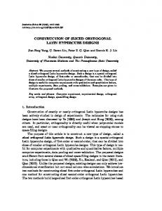
Figure 1.1: An NLHD based on the nested Latin hypercube in Table 1.1. The six points denoted by “+” consist of the nested smaller Latin hypercube design. For each dimension, each of the 24 equally spaced intervals of [0, 1) contains exactly one point and each of the six equally spaced intervals of [0, 1) contains exactly one point from the nested smaller design.

tive and qualitative factors. A nested Latin hypercube of 24 runs and a sliced Latin hypercube of 24 runs are given in Table 1.1. The NLHD and SLHD by coupling uniform random numbers are given in Figures 1.1 and 1.2, respectively. These NLHD and SLHD hold a special nested or sliced structure while achieving maximal uniformity in any one-dimensional projections as an OLHD. For a continuous function f , consider the numerical integration problem, ∫ µ = E{f (x)} =

f (x)dx [0,1)q

with q > 1. After evaluating f at a design of n runs, X1 , . . . , Xn , µ is estimated

A CLT FOR NESTED OR SLICED LH DESIGNS

3

Table 1.1: A nested Latin hypercube of 24 runs in two factors (left) and a sliced Latin hypercube of 24 runs in two factors (right). After mapping level x to ⌈x/4⌉, the six rows above the dashed line for the nested Latin hypercube become a Latin hypercube; and each of the four slices, separated by dashed lines for the sliced Latin hypercube, become a Latin hypercube with six runs.                                                     

5 22 10 16 4 20 17 9 24 11 14 21 7 12 13 2 8 1 18 19 23 15 3 6

1 23 7 15 10 19 12 18 3 22 6 14 20 5 16 24 9 4 13 8 21 11 2 17





                                                   

                                                   

5 13 9 3 21 17 1 20 8 16 10 22 18 4 6 11 15 23 12 2 24 7 14 19

3 21 19 11 16 8 9 24 7 17 4 13 6 18 14 2 23 10 22 5 20 15 1 12

                                                    

4

XU HE AND PETER Z. G. QIAN

0.6 0.4 0.0

0.2

Second dimension

0.8

1.0

An SLHD

0.0

0.2

0.4

0.6

0.8

1.0

First dimension

Figure 1.2: An SLHD based on the sliced Latin hypercube in Table 1.1. Points denoted by the same symbol consist of one slice of Latin hypercube design. For each dimension, each of the 24 equally spaced intervals of [0, 1) contains exactly one point and each of the six equally spaced intervals of [0, 1) contains exactly one point from each slice.

A CLT FOR NESTED OR SLICED LH DESIGNS

5

by µ ˆ = n−1

n ∑

f (Xi ).

(1.1)

i=1

Stein (1987) obtained a variance formula of µ ˆ from an OLHD that is no greater than the variance of an identically and independently generated sample of the same size. Similar formulas have been obtained for NLHD (Qian (2009)) and SLHD (Qian (2012)). The NLHD and SLHD have the same asymptotic variance as an OLHD of the same size. Methods for estimating the variance for OLHD are discussed in Stein (1987) and Owen (1992). Once the asymptotic variance is obtained, one can ask about the limiting distribution of µ ˆ. Owen (1992) obtained a central limit theorem for OLHDs. In this work, we show that µ ˆ in (1.1), computed from an NLHD or an SLHD, has the same limiting normal distribution as that for an OLHD. Our approach is conceptually simple using the method of moments. The challenges here are the special structures of NLHDs and SLHDs. This type of technique was used in Owen (1992) and He and Qian (2014) for OLHD and orthogonal array based designs. But the steps are quite different. The derived results are useful for making confidence statements in numerical integration, stochastic optimization, and uncertainty quantification. One may also be interested in the mean estimate using the small design of an NLHD or one slice of an SLHD. As shown in Qian (2009, 2012), either of these two designs is an OLHD and follows the same variance formula and asymptotic normal distribution as derived in Stein (1987) and Owen (1992). Section 2 presents some sampling properties of OLHD, NLHD and SLHD. To derive a unified central limit theorem for all three designs, we express the conditional distribution of OLHD, NLHD, and SLHD in the same form using big O notation. Section 3 provides our main result. Section 4 concludes with some brief discussion. 2. Dependence structures of Latin hypercube designs A uniform permutation on a set of a numbers is randomly generated with all a! permutations equally probable. Let I() be the indicator function. For a real number x, let ⌊x⌋ be the largest integer no greater than x, ⌈x⌉ be the smallest

6

XU HE AND PETER Z. G. QIAN

integer no smaller than x, and the subdivision of x with length 1/z be δz (x) = [⌊zx⌋/z, (⌊zx⌋ + 1)/z). An OLHD (McKay et al., 1979) of n points in q factors is constructed as Xik = πk (i)/n − ηik /n,

(2.1)

for i = 1, . . . , n and k = 1, . . . , q, where Xik is the kth dimension of Xi , the πk are uniform permutations on {1, . . . , n}, the ηik are generated from uniform distributions on (0, 1], and the πk and the ηik are generated independently. Proposition 1 follows from the construction. Unless noted otherwise, proofs are given in the supplementary materials. Proposition 1. Let X1 , . . . , Xn be constructed from an OLHD by (2.1) and take s ≤ n. The conditional density of Xs given X1 , . . . , Xs−1 is

=

gOLHD (d1 , . . . , dq )  0, {n/(n − s + 1)}q ,

dk ∈ δn (Xik ) for an 1 ≤ i ≤ s − 1, 1 ≤ k ≤ q, (2.2) otherwise.

An NLHD of n runs in q factors that contains a smaller Latin hypercube design with m runs and n = ml is constructed as Xik = ζk (π(i))/n − ηik /n,

(2.3)

for i = 1, . . . , n and k = 1, . . . , q, where Xik is the kth dimension of Xi . Here,  γ (i)l − τ k , i = 1, . . . , m, k i ζk (i) = ψ(ρ (i − m)), i = m + 1, . . . , n, k with π a uniform permutation on {1, . . . , n}, the γk uniform permutations on {1, . . . , m}, the τik generated from {0, . . . , l −1} with equal probabilities, the ψ(z) denote the zth element of {1, . . . , n}\{γk (j)l −τjk : j = 1, . . . , m}, the ρk uniform permutations on {1, . . . , n − m}, the ηik generated from uniform distributions on (0, 1], and π, the γk , the τik , the ρk and the ηik are generated independently. For i = 1, . . . , n, let Zi = 1 if π(i) ∈ {1, . . . , m} and Zi = 2 otherwise. Then the m rows with Zi = 1 form the smaller Latin hypercube design. The conditional density from an NLHD is more complicated than that for OLHD.

7

A CLT FOR NESTED OR SLICED LH DESIGNS

Proposition 2. Let X1 , . . . , Xn be constructed from an NLHD by (2.3) and take s ≤ n. Then the conditional density of Xs given X1 , . . . , Xs−1 , Z1 , . . . , Zs is gNLHD (d1 , . . . , dq )   0, dk ∈ δn (Xik ) for an 1 ≤ i ≤ s − 1, 1 ≤ k ≤ q,        0, Zs = 1, dk ∈ δm (Xik ) for an 1 ≤ i ≤ s − 1, 1 ≤ k ≤ q   = (2.4) such that Zi = 1,   ∏  q   other cases with Zs = 1,  k=1 gk (dk ),    ∏  q h (d ), other cases with Z = 2, s k=1 k k where gk (dk ) = ml/(m − |{i : 1 ≤ i ≤ s − 1, Zi = 1}|)/(l − |{i : 1 ≤ i ≤ s − 1, dk ∈ δm (Xik )}|), n(l − 1 − |{i : 1 ≤ i ≤ s − 1, dk ∈ δm (Xik ), Zi = 2}|) hk (dk ) = . (n − m − |{i : 1 ≤ i ≤ s − 1, Zi = 2}|)(l − |{i : 1 ≤ i ≤ s − 1, dk ∈ δm (Xik )}|) An SLHD (Qian (2012)) of n runs in q factors that can be divided into l slices of m points is constructed as Xik = ζk (π(i))/n − ηik /n,

(2.5)

for i = 1, . . . , n and k = 1, . . . , q, where Xik is the kth dimension of Xi , ζk (bm + a) = γbk (a)l − τγkk (a) (b), b

for a = 1, . . . , m and b = 0, . . . , l − 1, π is a uniform permutation on {1, . . . , n}, the γbk are uniform permutations on {1, . . . , m}, the τak are uniform permutations on {0, . . . , l − 1}, the ηik are generated from uniform distributions on (0, 1], and π, the γbk , the τak and the ηik are generated independently. For i = 1, . . . , n, let Zi = b if bm + 1 ≤ π(i) ≤ (b + 1)m. Then the m rows with the same value of Z consist of one slice of the sliced Latin hypercube design. Parallel to Proposition 2, Proposition 3 gives the conditional density from an SLHD. Proposition 3. Let X1 , . . . , Xn be constructed from an SLHD by (2.5) and take

8

XU HE AND PETER Z. G. QIAN

s ≤ n. Then the conditional density of Xs given X1 , . . . , Xs−1 , Z1 , . . . , Zs is gSLHD (d1 , . . . , dq )    0, dk ∈ δn (Xik ) for an 1 ≤ i ≤ s − 1, 1 ≤ k ≤ q,     0, dk ∈ δm (Xik ) for an 1 ≤ i ≤ s − 1, 1 ≤ k ≤ q = (2.6)   such that Z = Z , s i     ∏q g (d ), otherwise, k=1 k k where gk (dk ) = ml/(m−|{i : 1 ≤ i ≤ s−1, Zi = Zs }|)/(l−|{i : 1 ≤ i ≤ s−1, dk ∈ δm (Xik )}|). An OLHD can be seen as a special case of NLHD or SLHD with l = 1 and n = m. Propositions 1, 2 and 3 suggest that, although the three types of designs have different conditional densities, they share several properties. The densities are close to one in the majority of areas; the exception is when dk ∈ δm (Xik ) or dk ∈ δn (Xik ) for some i and k. The total volume of such subdivision areas has order O(n−1 ) as n goes to infinity. If we divide [0, 1)q into nq equally spaced squares, then the densities are uniform in each of the squares. We summarize these properties in the following. Proposition 4. Take s ≤ m. Let Msk be an s × s zero-one matrix whose (i, j)th element is one if and only if ⌊mXik ⌋ = ⌊mXjk ⌋ and Ms = (Ms1 , . . . , Msq ). Let X1 , . . . , Xn be generated from an OLHD in (2.1), an NLHD in (2.3), or an SLHD k ) in (2.5). Let Dik = δm (Xik ) for i = 1, . . . , s − 1 and k = 1, . . . , q, Dik = δn (X−i k for i = −(s − 1), . . . , −1 and k = 1, . . . , q, and D0k = [0, 1) \ ∪s−1 j=1 δm (Xj ) for

k = 1, . . . , q. Then the conditional density of Xs given X1 , . . . , Xs−1 , Z1 , . . . , Zs is g(d1 , . . . , dq ) =

s−1 ∑

bs (i1 , . . . , iq )I(d1 ∈ Di11 , . . . , dq ∈ Diqq ),

(2.7)

i1 ,...,iq =−(s−1)

where, for the sampling method OLHD, NLHD or SLHD, bs (i1 , . . . , iq ) is a deterministic function on n, m, i1 , . . . , iq , Z1 , . . . , Zs , Ms−1 , bounded as n goes to infinity, and bs (0, . . . , 0) = 1 + O(n−1 ). These conditional densities are expressed as sums of identity functions with weights. Note that (2.7) can be simplified for OLHD in that bs (i1 , . . . , iq ) is

A CLT FOR NESTED OR SLICED LH DESIGNS

9

irrelevant to Z1 , . . . , Zs , Ms−1 , and bs (i1 , . . . , iq ) = 0 if there is a k such that ik < 0. Using the overlapping domains of identity functions makes it possible to write the densities as a sum; using big O notation can unite the densities into one formula.

In each dimension, the identity function is depen-

dent on at most one of X1 , . . . , Xs−1 . The weights, although dependent on n, m, X1 , . . . , Xs−1 , Z1 , . . . , Zs , Mt−1 , are bounded as n goes to infinity. These new expression of the conditional densities simplifies the complicated dependence structure of three types of Latin hypercube designs and is convenient for deriving a central limit theorem. The expression is also useful for deriving a CLT of other types of designs when (2.7) holds. 3. A central limit theorem We first introduce the functional analysis of variance decomposition (Owen, (1994)) and variance formulas of Latin hypercube designs. Let F be the uniform ∏ measure on [0, 1)q with dF = qk=1 dF{k} , where F{k} is the uniform measure on [0, 1). Assume f is a continuous function on [0, 1]q and with finite variance ∫ f (x)2 dF . Express f as ∑ f (x) = µ + fu (x), ϕ⊂u⊆{1,...,q}

where µ =

∫

f (x)dF and fu is defined recursively via ∫ ∑ fu (x) = {f (x) − fv (x)}dF{1,...,q}\u . v⊂u

If u ∩ v ̸= ϕ,

∫ fu dx = 0.

(3.1)

v

Let αk (x) = f{k} (x). The remaining part, r(x), of f is f (x) = µ +

q ∑

αk (x) + r(x).

(3.2)

k=1

From Stein (1987), as n goes to infinity, the variance of µ ˆ in (1.1) of an OLHD is ∫ var(ˆ µ) = n−1 r(X)2 dF (X) + o(n−1 ). The same formulas obtain for NLHDs (Qian (2009)) and SLHDs (Qian (2012)). Here is a result on the method of moments (Durrett (2010)).

10

XU HE AND PETER Z. G. QIAN

Lemma 5. Let A1 , A2 , . . . be random variables with distribution functions F1 , F2 , . . . so that for any p = 1, 2, . . . and n = 1, 2, . . ., ∫ +∞ (p) mn = xp dFn −∞

is finite. Let F be a distribution function with finite moments for which { } lim sup (m(2p) )1/2p /(2p) < ∞. p→∞

(p)

If for any p = 1, 2, . . ., limn→∞ mn = m(p) , then An converges in distribution to F . We state two useful lemmas that parallel results for ordinary Latin hypercube designs in Owen (1992). Let |D| be the volume of region D. Let EIID be the expectation of a function with an identically and independently sample. Lemma 6. For any continuous function f on [0, 1]q and fixed l, as n → ∞, E{f (Xs ) | X1 , . . . , Xs−1 } = EIID {f (Xs )} + O(n−1 ), where the first expectation is over an OLHD in (2.1), an NLHD in (2.3) or an SLHD in (2.5). Lemma 7. Let ¯ = n−1 R

n ∑

r(Xi ),

i=1

where r(x) is the remaining part by (3.2) of a continuous function f on [0, 1]q . Then for any positive integer p and fixed l, as n → ∞, ¯ p } = EIID {(n1/2 R) ¯ p } + o(1), E{(n1/2 R) where the first expectation is over an OLHD in (2.1), an NLHD in (2.3), or an SLHD in (2.5). Theorem 8. Suppose f is a continuous function from [0, 1]q to R, µ ˆ in (1.1) is based on X1 , . . . , Xn generated from an OLHD, NLHD, or SLHD. Then, as n → ∞, n

1/2

( ∫ ) 2 (ˆ µ − µ) → N 0, r(x) dx .

A CLT FOR NESTED OR SLICED LH DESIGNS

11

Proof. The mean of n1/2 (ˆ µ − µ) is 0 and the variance of n1/2 (ˆ µ − µ) tends to ∫ 2 r(x) dx. From Lemma 7, for p = 1, 2, . . ., ¯ p } = EIID {(n1/2 R) ¯ p } + o(1). E{(n1/2 R) ¯ follows a When the points are generated identically and independently, n1/2 R ∫ normal distribution with mean zero and variance σ 2 = r(x)2 dx. From Owen (1980),

{ ¯ p} = EIID {(n1/2 R)

0, σ p (p

p = 1, 3, 5, . . . , − 1)!!, p = 2, 4, 6, . . . .

¯ from an Thus lim supp→∞ (σ p (p − 1)!!)1/p /p = 0 and, from Lemma 5, n1/2 R OLHD, an NLHD or an SLHD has the same normal limiting distribution as ¯ with the points generated identically and independently. n1/2 R We can easily extend Theorem 8 to a multivariate function f = (f1 , . . . , fp ). Parallel to (3.2), define ri (x) via fi (x) = µi +

q ∑

αi,k (x) + ri (x).

k=1

Corollary 9. Suppose f is a continuous function from [0, 1]q to R p , µ ˆ in (1.1) is based on X1 , . . . , Xn generated from an OLHD, NLHD or SLHD. Then, as n → ∞, n1/2 (ˆ µ − µ) → N (0, Σ), where Σ is a p × p matrix with the (i, j)th ∫ element Σi,j = ri (x)rj (x)dx. Proof. The normality of multivariate f follows from the fact that any linear combinations of (f1 , . . . , fp ) has a limiting normal distribution. As an example, take an NLHD and an SLHD with n = 24, m = 6, l = 4, and q = 2. We estimate the mean output µ of the Branin function (Branin (1972)) ( )2 ( ) 5.1 5 1 f = x2 − 2 x21 + x1 − 6 + 10 1 − cos(x1 ) + 10 4π π 8π on the domain [−5, 10] × [0, 15]. The true value of µ is approximately 54·31, ∑24 computed from a large grid. We computed µ ˆ = i=1 f (Xi )/24 for the two designs, repeated for 100000 times. The density plots of µ ˆ from the two designs are shown in Figure 3.3.

12

XU HE AND PETER Z. G. QIAN

0.04 0.03 0.00

0.01

0.02

Density

0.03 0.02 0.00

0.01

Density

0.04

0.05

An SLHD of 24 runs

0.05

An NLHD of 24 runs

30

40

50

60

Mean output

70

80

30

40

50

60

70

80

Mean output

Figure 3.3: Density plots (solid curves) of µ ˆ based on NLHDs (left) and SLHDs (right), both close to a normal distribution (dashed curves).

A CLT FOR NESTED OR SLICED LH DESIGNS

13

4. Conclusions A central limit theorem has been derived for nested or sliced Latin hypercube designs. It is shown that µ ˆ in (1.1) computed from a nested or sliced Latin hypercube design has the same limiting normal distribution as that of an ordinary Latin hypercube design. The derived results are useful for making confidence statements in numerical integration (Kuo, Schwab and Sloan (2011)), stochastic optimization (Birge and Louveaux, (2011); Shapiro, Dentcheva and Ruszczynski (2009)), uncertainty quantification (Xiu, 2010) and other applications. For extending our technique to derive central limit theorems for more general types of Latin hypercube designs, such as NLHD or SLHD of multiple layers or a mix of NLHD and SLHD, it remains a challenge to derive probabilistic structures of this general class of designs. Another problem for future research would be to allow l to go to infinity.

Supplementary Materials The supplementary materials contain the proofs of Propositions 1-4 and Lemma 7.

Acknowledgment The authors thank the Editor, an AE, and two referees for valuable comments which improved the article. He is partially supported by NSFC 11501550 and DOE DE-SC0010548. Qian is partially supported by National Science Foundation Grants CMMI 1233570 and DMS 1055214.

References Birge, J. R. and F. Louveaux (2011). Introduction to Stochastic Programming. Springer-Verlag, New York. Branin, F. K. (1972). A widely convergent method for finding multiple solutions of simultaneous nonlinear equations. IBM J. Res. Dev. 16, 504–22. Durrett, R. (2010). Probability: Theory and Examples. Cambridge University Press, Cambridge. He, X. and P. Z. G. Qian (2014). A central limit theorem for general orthogonal

14

XU HE AND PETER Z. G. QIAN

array based space-filling designs. Ann. Statist. 42, 1725–1750. Kuo, F. Y., C. Schwab, and I. H. Sloan (2011). Quasi-Monte Carlo method for high-dimensional integration: the standard (weighted Hilbert space) setting and beyond. Anziam Journal 53, 1–37. McKay, M. D., R. J. Beckman, and W. J. Conover (1979).

A comparison

of three methods for selecting values of input variables in the analysis of output from a computer code. Technometrics 21, 239–45. Owen, A. B. (1992). A central limit theorem for Latin hypercube sampling. J. R. Stat. Soc. B, 54, 541–51. Owen, A. B. (1994). Lattice sampling revisited: Monte Carlo variance of means over randomized orthogonal arrays. Ann. Statist. 22, 930–45. Owen, D. B. (1980). A table of normal integrals. Commun. Stat. Simulat. 9, 389–419. Qian, P. Z. G. (2009). Nested latin hypercube designs. Biometrika 96, 957–970. Qian, P. Z. G. (2012). Sliced latin hypercube designs. Journal of the American Statistical Association 107, 393–399. Shapiro, A., D. Dentcheva, and A. Ruszczynski (2009). Lectures on Stochastic Programming: Modeling and Theory. SIAM-Society for Industrial and Applied Mathematics, Philadelphia. Stein, M. (1987). Large sample properties of simulations using Latin hypercube sampling. Technometrics 29, 143–51. Xiu, D. (2010). Numerical Methods for Stocahstic Computations: A Spectral Method Approach. Princeton University Press, New Jersey.

Academy of Mathematics and Systems Science, Chinese Academy of Sciences, 55 East Zhongguancun Rd., Haidian Dist., Beijing 100190, China. E-mail: [email protected]

A CLT FOR NESTED OR SLICED LH DESIGNS

Department of Statistics, University of Wisconsin-Madison, 1300 University Avenue, Madison, WI 53706, USA. E-mail: [email protected]

15