A certification of Lagrange’s theorem with the proof assistant ÆtnaNova/Referee ⋆ Domenico Cantone, Salvatore Cristofaro, and Marianna Nicolosi Asmundo Dipartimento di Matematica e Informatica, Universit` a di Catania Viale A. Doria 6, I-95125 Catania, Italy e-mail: {cantone|cristofaro|nicolosi}@dmi.unict.it
Abstract. We report on the computerized verification of Lagrange’s theorem, carried out with the proof assistant ÆtnaNova/Referee. The scenario starts with the basic definitions in group theory, such as the notions of subgroups and right cosets. Then, the proof of Lagrange’s theorem is formalized following the same approach present in most algebra textbooks. The proof assistant ÆtnaNova/Referee is grounded on a variant of ZermeloFraenkel set theory, designed for the automatic verification of proofs. Referee is provided with a powerful inferential and defining mechanism based on set theory, together with a notation very close to that commonly used in mathematics. We also compare our set theoretic approach in the formalization of elementary group theory, and in particular of Lagrange’s theorem, with those followed in other, more widespread, proof assistants. Key words: automated proof verification, Lagrange’s theorem, set theory.
In memory of Jacob (Jack) T. Schwartz [January 9, 1930 - March 2, 2009]
1
Introduction
Proof assistants aim at the mechanical verification, or certification, of the correctness of fully formalized theorem and program correctness proofs [25]. Their approach is different from that of automated theorem provers, as they are provided with inference mechanisms to check proofs already engineered by humans, rather than proof search procedures and heuristics. Fully formalizing a mathematical proof and submitting it to a verifier results harder than just writing it by pencil and paper in the usual semi-formal style, since the user must develop the proof from scratch, specifying all details and including derivation steps, that are usually omitted in the semi-formal approach. However, once a formal proof has been checked by a proof assistant, it becomes ⋆
Work partially supported by MIUR project “Large-scale development of certified mathematical proofs” n. 2006012773.
certified proofware that can be reused in other proofs. Moreover, the great level of detail characterizing computerized proofs allows sometimes to point out certain aspects of the manipulated objects that in semi-formal proofs are usually hidden. In this paper we present a formalization of Lagrange’s theorem for algebraic group theory, which states that the order of every subgroup S of any finite group G divides the order of G (see [21] and Section 3). It turns out that our formalization closely parallels the semi-formal presentations of most algebra textbooks, such as, for instance [21]. After introducing the basic definitions of group identity and of the inverse operation, we prove some of their algebraic properties. Subsequently, the notions of subgroup and right coset of a subgroup are formalized and some related properties are proved as well. Finally, using such results, Lagrange’s theorem is proved. The verifier we used to check the above outlined proof scenario is ÆtnaNova/Referee [18], which is grounded on a variant of Zermelo-Fraenkel set theory designed for the automatic verification of proofs.1 Referee comprises a powerful inferential and defining mechanism based on set theory. Scenarios are written in a set theoretic language very close to that one commonly uses in mathematics. The current implementation of Referee has been developed together with a challenging proof scenario, not yet complete, that starting from the barest rudiments of set theory aims at proving Cauchy’s Integral theorem for analytic functions. The adoption of set theory to formalize mathematical notions and to reason on them makes Referee different from most of the proof assistants currently in use, usually based on a logic calculus on which mathematical theories (such as set theory itself) are defined. The verifiers HOL [13] and Isabelle [17], for instance, are based on higher-order logic, Mizar [15] on first-order logic and set theory, and the proof assistant Coq [2] on a variant of the lambda calculus called the Calculus of Inductive Constructions. Several researchers working on the development of the proof systems mentioned above have been interested in the formalization of group theory. In [1], group theory has been formalized from scratch up to the proof of Lagrange’s theorem. Mizar’s library contains a number of articles treating several results in group theory [16]. The certification of the first Sylow’s theorem with the verifier Isabelle HOL has been presented in [14], whereas [12] provides a formalization of finite group theory including Sylow’s theorems verified by the Coq proof assistant. Such efforts are partly motivated by the need of producing proofware for a generic theory, such as group theory is, so as it can be reused in the context of more complex or specific theories. Additionally, group theory includes theorems with long and complex semi-formal proof (as for instance Feit-Thompson theorem, whose original proof is 274 pages long [8]), that constitute real challenges for proof verifiers. 1
The interested reader can access the system by asking for an account to the administrator of Referee:
[email protected].
Thus, our contribution besides the primary goal of providing a formalization of group theory, and in particular of Lagrange’s theorem, to be reused in other Referee proof scenarios, has the additional goal of comparing our approach with the ones pursued in other, more widespread, proof assistants.
2
ÆtnaNova/Referee
ÆtnaNova/Referee is an automatic tool that can be used online to check the correctness of mathematical proofs. Fragments of mathematics to be checked for correctness are formalized in a set theoretic language, very close to the everyday standard mathematical language, put in scripts, and submitted to the verifier. If the verification task succeeds, the formal scenario is certified as valid proofware, that may be reused in the context of other proof scenarios. Otherwise it is rejected and a suitable diagnostic file is returned to the user. Currently, Referee is a working prototype written in SETL2, a high-level programming language based on set primitives [23]. Referee is being extensively tested through the development of several proof scenarios in mathematics, as the ones illustrated in [19, 6] concerning such foundational notions as pairs, maps, ordinals, inductive sets, the set of real numbers, and so on. We cite also some proof scenarios in computer science, as the ones described in [18, 20] concerning the correctness of a bisimulation algorithm and of the Davis-Putnam procedure, respectively. All proofware checked by Referee is stored in a common scenario ready to be reused when needed in the development of other proofs. The specification language and deductive apparatus of the verifier are grounded on a version of Zermelo-Fraenkel set theory which employs, together with the usual set theoretic operators, constructs designed to assist in the formal development of proofs. The reason behind this choice is to take advantage of the great expressive power of set theory, that, taking sets as primitive objects is in fact a proper ground on which to construct the whole mathematics. Even notions such that of integer numbers, considered primitive by other proof assistants, are reduced to sets, following von Neumann’s approach. Set theory can also be used to represent, by means of suitable operations, various constructs of symbolic languages, such as logic and programming languages. Such characteristic has shown to be very useful in the development of proof scenarios in computer science. For instance, in [20], classical results on the representation of propositional formulae in CNF by means of sets of clauses, have been employed to check the correctness of the Davis-Putnam decision procedure. In this section we illustrate a few features of the Referee verifier, specifically those which have been employed within the proof scenario of our interest. For a more detailed account on Referee and on its definitional and inferential mechanisms, the reader is referred to [18, 19] and to the online book draft [22]. 2.1
Formalization and definition tools
The language used to formalize definitions and proofs to be given in input to the verifier contains the usual set theoretic operators. Among them we mention the
binary operations of union ∪, intersection ∩, and set difference \. The singleton operator X 7−→ {X} is also available to define nested sets. Unordered lists can be defined as {X1 , . . . , Xn } =Def {X1 } ∪ . . . ∪ {Xn }. Ordered pairs are definable in several ways. The definition used in our scenario, due to J.T. Schwartz, is illustrated in Fig. 1 (cf. Def 1). Ordered tuples are plain extensions of ordered pairs. Some useful operations derived from the basic set theoretic operations are: X with Y := X∪{Y } (yields a set whose elements are those of X plus the element Y ), X less Y := X \ {Y } (removing Y from X), and next(X) := X with X. By repeated applications of the latter operation, one can build the natural numbers a ` la von Neumann, starting from the empty set ∅ (regarded as the natural number 0). The selection of an element from a set X is executed by the global choice function arb, which satisfies the properties arb(∅) = ∅, arb(X) ∈ next(X) and X ∩ arb(X) = ∅, for all X. As illustrated in Fig. 1, the above mentioned operators suffice to define the notions of ordered pairs and of the extractors of their first and second components.
Def 1: [Ordered pair] Def([X,Y]) := {{X},{{X},{{Y},Y}}} Def 2: [First component of ordered pair] car(X) := arb(arb(X)) Def 3: [Second component of ordered pair] cdr(X) := arb(arb(arb(X - {arb(X)}) {arb(X)}))
Fig. 1. Definition of ordered pairs and of their extractor functions.
Set formers are defined in the general form {e : x0 C0 t0 , x1 C1 t1 , . . . , xn Cn tn | ϕ}, where each Ci is either the ∈ relation or the ⊆ relation, e and ϕ are respectively a set-term and a condition in which the xi s may occur free.2 Set formers allow one to define operations such as the general union, the powerset and the Cartesian product. Formal definitions of maps, of single-valued maps, and of one-to-one maps can plainly be built up from the definition of ordered pairs and from the set former construct. Their definition, as formalized in the common scenario, is reported in Fig. 2 (notice that the symbol •imp stands for the classical logical implication →). 2
Given a denumerable collection of variables, the constant symbol ∅, the binary set theoretic operations ∪, ∩, \, the singleton operation {·}, and the relation symbols ∈, =, and ⊆, set-terms can be defined inductively as follows: Each variable is a set-term, and the constant ∅ is a set-term; e1 ∪e2 , e1 ∩e2 , e1 \e2 , and {e1 } are set-terms, for any two given set-terms e1 and e2 ; set formers are set-terms. Conditions are first-order set theoretic formulae that may contain set-terms and the predicates ∈ and ⊆.
-----
Next we define various familiar notions of set theory: (possibly multivalued) maps, their ranges and domains, and the subclasses of single-valued and 1-1 maps. After giving these definitions we build up a few small utility theories which ease subsequent work with these predicates.
Def 4: [Is-a-map predicate] Is map(F) := F = {[car(x), cdr(x)]: x in F} Def 5: [Map domain] Domain(F) := {car(x): x in F} Def 6: [Map range] Range(F) := {cdr(x): x in F} Def 7: [Single-valued map predicate] Svm(F) := Is map(F) & (FORALL x in F, y in F | (car(x) = car(y)) •imp (x = y)) Def 8: [One-one map predicate] One 1 map(F) := Svm(F) & (FORALL x in F, y in F | (cdr(x) = cdr(y)) •imp (x = y))
Fig. 2. Formal definitions related to maps.
The set theoretic axioms of extensionality, choice, infinity, and replacement are built-in in the version of set theory underlying the Referee system. This, as mentioned earlier, is also provided with a defining mechanism, called THEORY, which allows to define new symbols. The THEORY construct is also useful to modularize scenarios and for proofware reuse. Theories defined by the THEORY construct can be seen as procedures of a programming language. In fact, they are provided with a list of formal parameters that are required to satisfy certain assumptions. Once a theory T is specified, it can be used in the scenario by the command ENTER THEORY T. It is possible to use the assumptions of the current theory in the scenario by the primitive Assump. Once a theory has been defined, it can be applied using new parameters satisfying the assumptions of the theory. The primitive devoted to such a task is APPLY. 2.2
Deduction mechanisms
In Referee, proofs are developed in a “natural deduction” style. This involves the formulation of temporary assumptions that are successively discarded. In particular, theorems are proved by contradiction, namely by attempting at deriving absurd consequences from their negations. The inferential apparatus of Referee comprises fifteen deduction rules. Among them we mention the primitives ELEM, Suppose not, EQUAL, and Use def. We will briefly discuss all of them later in this section. A proof is a sequence of statements, also called inferential steps, each of which consists of three parts: a hint indicating which deduction rule to invoke, the sign ==>, and the assertion of the statement, a well-formed formula in the set theoretic language of Referee which has to be deduced by the chosen deduction rule in its own context. If not otherwise specified, the context of an occurrence of a rule within a proof is constituted by all the assertions preceding it in the proof. It is possible (and sometimes needed for efficiency reasons) to reduce the context of an occurrence of a rule by labeling the assertions actually needed by the rule to carry out its derivation (see for example the reduction of context of
the occurrence of the ELEM primitive at line 28 of the formal proof of Theorem trcb18 in Fig. 8, Section 4). Among the deduction rules provided by Referee, ELEM is the most important one. It implements in an efficient way an optimized decision procedure (cf. [4, 7]) for the satisfiability problem for a variant of the multilevel syllogistic with singleton, called MLSS. MLSS is an unquantified fragment of set theory consisting of a denumerable infinity of set variables, the null set constant ∅, the binary set operators ∪, ∩, and \, the set predicates ∈, =, and ⊆, and the propositional connectives. The semantics of MLSS is based upon the von Neumann cumulative hierarchy of sets. The satisfiability problem for MLSS consists in determining whether or not any given MLSS-formula ϕ is satisfiable. A first decision procedure was presented in [9]. Subsequently, it was shown that the satisfiability problem for conjunctions of ‘flat’ MLSS-literals of the forms x = y, x 6= y, x ∈ y, x ∈ / y, x = y ∪z, x = y \z, x = {y}, to be called normalized MLSS-conjunctions, is NP-complete (cf. [5]); more recently, its decision procedure was optimized in [4, 7] by means of semantic tableaux. The Suppose not primitive occurs exclusively and always as a hint of the first statement of a proof. It usually has the form Suppose not(c1,..,cn) ==>... where c1,..,cn are parameters (local to the proof), corresponding in number and position to the (universally quantified) variables of the statement of the theorem. Suppose not(c1,..,cn) negates the statement of the theorem and instantiates its variables (now existentially quantified) with the parameters c1,..,cn. The assertion at the right of Suppose not is allowed to be any well-formed formula logically equivalent to the negation of the statement of the theorem instantiated with the parameters c1,..,cn. At the end of the proof there must appear a statement of the form Discharge ==> QED. Two further primitives are EQUAL and Use def. The EQUAL deduction rule works as follows: it takes into account all the equalities of the form s = t, where s and t are terms which have been derived in the context K of the rule, and propagates them transitively within all terms and formulae occurring in K. Use def substitutes each occurrence of a previously defined function or predicate symbol present in the assertions of its context with its actual definition. The resulting context is then used as the basis for an ELEM deduction.
3
A brief outline of group theory
Next we briefly outline some basic concepts of group theory used in the formalization of Lagrange’s theorem. For further details the reader is referred to textbooks as [21]. A group is an ordered pair (G, mult) where G is a nonempty set and mult is a binary function (called multiplicative operation) satisfying the following properties: (A1) Closure: (∀x ∈ G)(∀y ∈ G)(mult(x, y) ∈ G)
(A2) Associativity: (∀x ∈ G)(∀y ∈ G)(∀z ∈ G)(mult(x, mult(y, z)) = mult(mult(x, y), z)) (A3) Existence of left identity and left inverse: (∃e ∈ G)((∀x ∈ G)(mult(e, x) = x) ∧ (∀x ∈ G)(∃y ∈ G)(mult(y, x) = e)) A left identity of a group (G, mult) is an element e ∈ G such that mult(e, x) = x, for all x ∈ G. If e is a left identity of (G, mult) and x, y ∈ G, we say that y is a left inverse of x relative to e if mult(y, x) = e. By (A3), a left identity e exists, and every element x ∈ G has a left inverse relative to e. It can easily be shown that the left identity of a group (G, mult) is uniquely determined. Similarly, for each element x ∈ G there is exactly one y ∈ G which is a left inverse of x relative to e. We call e the identity of (G, mult) and, for each x ∈ G, we call the (unique) left inverse of x relative to e the inverse of x. From now on, we denote the identity of a group (G, mult) with identity and the inverse of an element x ∈ G with inverse(x). Let (G, mult) be a group and S a nonempty subset of G, then S is a subgroup of (G, mult) if S is closed under the operations mult and inverse. If S is a subgroup of (G, mult) and t ∈ G, the right coset of S with representative t is the set RightCoset(S, t) = {mult(x, t) : x ∈ S}. The set of all right cosets of S is denoted with RightCosets(S), i.e., RightCosets(S) = {RightCoset(S, t) : t ∈ G} . A group (G, mult) is finite if G is a finite set. In such a case the number of elements of G is called the order of (G, mult) and denoted by |G|. (In general, given any finite set X we denote with |X| the cardinality of X, i.e., the number of elements of X.) Trivially, if (G, mult) is finite and S is a subgroup of (G, mult), then S is also finite. Moreover, S has also a finite number of right cosets, and RightCosets(S) = {RightCoset(S, t1 ), . . . , RightCoset(S, tn )}, where G = {t1 , . . . , tn }. The number of right cosets of S is called the index of S (in G) and is denoted by [G : S], i.e., [G : S] = |RightCosets(S)| (see [21]). Using the above definitions, we can formally state Lagrange’s theorem as follows (see [21]): Theorem 1 (Lagrange’s theorem). Let (G, mult) be a finite group and let S be a subgroup of (G, mult). Then |S|·[G : S] = |G|, thus the order of the subgroup (S, mult) divides the order of (G, mult).
4
A proof scenario on Lagrange’s theorem
Our proof scenario of Lagrange’s theorem consists of a theory, called group, whose input parameters, G and mult, have to satisfy the assumptions presented in Fig. 3. These are formalizations of the properties of groups (A1), (A2), and (A3), given in Section 3. The complete proof scenario can be found at the URL: http://www.dmi.unict.it/∼cantone/Referee/Lagrange.txt . It consists of 1120 lines of proofware (including comments), 76 theorems and 20 symbol definitions. Referee verifies the scenario in 6 seconds (on average).
THEORY group(G, mult(x,y)) -- Closure properties (FORALL x, y | ((x in G) & (y in G)) •imp (mult(x,y) in G)) -- Associativity (FORALL x, y, z | (((x in G) & (y in G)) & (z in G)) •imp (mult(x,mult(y,z)) = mult(mult(x,y),z))) -- Existence of left identity and left inverse (EXISTS E | (E in G) & (FORALL X | (X in G) •imp (mult(E,X) = X)) & (FORALL X | (X in G) •imp (EXISTS Y | (Y in G) & (mult(Y,X) = E)))) END group
Fig. 3. The assumptions of the theory group.
4.1
Preliminary definitions and properties
Initially, some basic notions of group theory are formally defined and introduced in the theory group. Among them, in particular, we mention the notions of the identity and of the inverse function of a group. Their formalizations, which make use of the set former and of the arb operator, are reported in Fig. 4. The formalization of the identity deserves a few comments. After introducing
-- An element E of the group G is an identity (of G) if mult(X,E) = X, for all X in G. -- We define the predicate "is identity(E)" to mean that E is an identity. Def dg1: is identity(E) := (FORALL X | (X in G) •imp (mult(E,X) = X)) -- The set of all identities is defined by: Def dg2: identities := {E in G | is identity(E)} -- Using the choice operator "arb" we define the identity of the group G. Def dg3: identity := arb(identities) -- Given an element X of the groups G, an inverse of X is an element Y of G such that -- mult(Y,X) is an identity. -- We define the predicate "is inverse(X,Y)" as follows: Def dg4: is inverse(X,Y) := is identity(mult(Y,X)) -- The set of the inverses of X is denoted by "inverses(X)". Def dg5: inverses(X) := {Y in G | is inverse(X,Y)} -- Using the choice operator "arb" we define the inverse of an element X of the group -- G. Def dg6: inverse(X) := arb(inverses(X))
Fig. 4. The basic definitions of identity and inverse.
the predicate is identity(e) ⇔Def (∀x ∈ G)(mult(e, x) = x) (Def dg1), which provides the defining property of group identity in (G, mult), we then define the set identities =Def {e ∈ G | is identity(e)} (Def dg2), representing the collection of all the identities of (G, mult). Finally, using the global choice operator arb (Def
dg3), we define the identity of a group (G, mult), as an “arbitrary” element of the set identities (formally, identity =Def arb(identities)). The formalization of the inverse operation, described through Defs dg4-dg6 in Fig. 4, follows along similar lines. It is then checked that the notions of identity and of inverse are correctly formalized, in the sense that identity and inverse, as defined above, satisfy some important basic properties such as the one stating that mult(x, identity) = mult(identity, x) = x and mult(inverse(x), x) = mult(x, inverse(x)) = identity, for all x ∈ G. It is also certified that both identity and inverse(x), for every x ∈ G, are uniquely determined. Many other elementary algebraic properties of the identity and the inverse operation are formalized and proved as well. These include, for instance, the following ones: Uniqueness of idempotent elements: if x ∈ G and mult(x, x) = x, then x = identity; Double inverse: if x ∈ G then inverse(inverse(x)) = x; Inverse of the multiplication: if x, y ∈ G then inverse(mult(x, y)) = mult(inverse(y), inverse(x)); Cancellation law: if x, y, z ∈ G and mult(x, z) = mult(y, z) then x = y. The basic tools for the formalization of the proof of Lagrange’s theorem include, together with the notions and properties reported above, the definitions of subgroup and right coset, whose formalization is illustrated in Fig. 5 (the symbol •incin in Definition dg7 stands for the set inclusion ⊆ symbol).
-- A subgroup (of G) is a nonempty subset S of G which is closed under the operations -- mult and inverse of G. -- The predicate "subgroup(S)" denotes the fact that S is a subgroup (of G). Def dg7: subgroup(S) := (S /= 0) & (S •incin G) & (FORALL x, y | (((x in S) & (y in S)) •imp (mult(x,y) in S))) & (FORALL x | ((x in S) •imp (inverse(x) in S))) -- Given a subgroup S (of G) and an element T of G, the right coset of S with -- representative T is the set of all elements of the form mult(X,T), where X belongs -- to S. Def dg8: RightCoset(S,T) := {mult(X,T) : X in S} -- The set of all right cosets of a subgroup S. Def dg9: RightCosets(S) := {RightCoset(S,T) : T in G}
Fig. 5. The definitions of subgroups and right cosets.
-- Now we turn to Lagrange’s theorem. -- We define explicitly a function "RCB(S)" such that, for any subgroup S, RCB(S) is a -- map whose domain is the Cartesian product of S with the set of the right cosets -- of S, and whose range is the group G. -- The definition of RCB(S) follows: Def dg10: RCB(S) := {[[X,R],mult(X,arb(R))] : X in S, R in RightCosets(S)}
Fig. 6. The formal definition of set RCB(S).
4.2
The main result
Let us consider the following three facts: (a) for every subgroup S of (G, mult), the set RightCosets(S) of the right cosets of S is a partition of G, (b) every right coset of a subgroup S of (G, mult) is equipollent to S itself,3 and (c) if P is a partition of a set X and any set belonging to P is equipollent to a (fixed) set Y , then the Cartesian product Y × P is equipollent to X. One could first show separately that the facts (a), (b), and (c) hold, and then prove Lagrange’s theorem as a plain consequence of them. In fact, from (a), (b), and (c), it follows immediately that (i) S × RightCosets(S) is equipollent to G. Additionally, we have (ii) |A × B| = |A| · |B|. Thus, if (G, mult) is a finite group, the sets G, S, and RightCosets(S) are all finite, and hence, by (i), |S×RightCosets(S)| = |G|. Therefore, by (ii), we have that |S|·|RightCosets(S)| = |G|, i.e., |S| · [G : S] = |G| which is just the conclusion of Lagrange’s theorem. The approach just outlined is basically the same adopted in most algebra textbooks (see for instance [21]). In our proof scenario we followed it as well, but with some slight differences which made the overall proof process a little bit simpler. Specifically, we showed that (i) can be proved without using (b) and (c). To do so, it is convenient to define the following set RCB(S) =Def {[[x, R], mult(x, arb(R))] | x ∈ S, R ∈ RightCosets(S)} , whose formal definition within Referee is reported in Fig. 6. It turns out that RCB(S) is in fact a one-to-one map whose domain is the Cartesian product S × RightCosets(S) and whose range is G, thus implying immediately (i). To begin with, one first derives that RCB(S) is a single-valued map and that Domain(RCB(S)) = S × RightCosets(S), from the very definition of RCB(S). The proof that Range(RCB(S)) ⊆ G holds can be formalized starting from the first assumption in the theory group (see Fig. 4) and from the following two facts: – S ⊆ G, and 3
We recall that, by definition, a set A is equipollent to a set B if and only if there exists a one-to-one correspondence f from A onto B.
– ∅ ⊂ R ⊆ G and arb(R) ∈ R, for all R ∈ RightCosets(S), by introducing only a few simple intermediate lemmas. The most complicated part consists in proving formally that G ⊆ Range(RCB(S)) (this, together with the fact that Range(RCB(S)) ⊆ G, implies that Range(RCB(S)) = G) and that RCB(S) is one-to-one. These results have been established by developing the formal proof of a consistent number of properties of subgroups and of right cosets of a subgroup. A complete description of a formal proof. We devote the last part of the present section to the description of a formal proof that RCB(S) is a one-to-one map. In view of the definition of one-to-one maps given in Fig. 2, such proof consists in proving that – RCB(S) is a single-valued map, and that – if A, B ∈ RCB(S) and cdr(A) = cdr(B), then A = B. We focus on the second statement, which is formalized by Theorem trcb18 reported in Fig. 8, whose semi-formal proof is given next. Semi-formal proof of Theorem trcb18. We must show that if A, B ∈ RCB(S) and cdr(A) = cdr(B), then A = B. Assume, by way of contradiction, that this is not the case, i.e., that A, B ∈ RCB(S), cdr(A) = cdr(B), but A 6= B. By the definition of RCB(S) we have that A = [[x1 , r1 ], mult(x1 , arb(r1 ))] and B = [[x2 , r2 ], mult(x2 , arb(r2 ))], where x1 , x2 ∈ S and r1 , r2 ∈ RightCosets(S). Therefore, since cdr(A) = cdr(B), it follows that mult(x1 , arb(r1 )) = mult(x2 , arb(r2 )) . (1) At this point we use the following two properties, whose proofs have been formalized in the scenario as well (see Fig. 7): Property 1: If R ∈ RightCosets(S), y ∈ R, and x ∈ S, then mult(x, y) ∈ R. Property 2: If X, Y ∈ RightCosets(S) and X ∩ Y 6= ∅, then X = Y .4 In fact, from Property 1 it follows that mult(x1 , arb(r1 )) ∈ r1
and mult(x2 , arb(r2 )) ∈ r2
and hence, using (1) above, we get that r1 ∩ r2 6= ∅. From this, using Property 2, we obtain that r1 = r2 and therefore arb(r1 ) = arb(r2 ). Thus, by putting x = arb(r1 ) = arb(r2 ), by (1) again we have that mult(x1 , x) = mult(x2 , x) and hence, by the cancellation law, we get x1 = x2 . Summing up, we have shown that x1 = x2 and r1 = r2 , which imply that A = B, contradicting the assumption that A 6= B. Hence RCB(S) must be one-to-one. 4
The proof of these two properties can be found in most common textbooks of group theory. For instance, property (2) corresponds to Theorem 2.9 of [21].
Theorem trcb1: (subgroup(S) & (R in RightCosets(S)) & (X in S) & (Y in R)) •imp (mult(X,Y) in R). Theorem tp2: (subgroup(S) & (X in RightCosets(S)) & (Y in RightCosets(S)) & ((X * Y) /= 0)) •imp (X = Y).
Fig. 7. The formalized statements of Property 1 and Property 2, as Theorems trcb1 and tp2, respectively.
1. 2. 3. 4. 5. 6. 7. 8. 9. 10. 11. 12. 13. 14. 15. 16. 17. 18. 19. 20. 21. 22. 23. 24. 25. 26. 28. 29. 30. 31. 32.
Theorem trcb18: (subgroup(S) & (A in RCB(S)) & (B in RCB(S)) & (cdr(A) = cdr(B))) •imp (A = B). Proof: Suppose not(s,a,b) ==> subgroup(s) & (a in RCB(s)) & (b in RCB(s)) & (cdr(a) = cdr(b)) & (a /= b) Use def(RCB) ==> Stat0: (a in {[[X,R],mult(X,arb(R))] : X in s, R in RightCosets(s)}) (x1,r1)-->Stat0 ==> (x1 in s) & (r1 in RightCosets(s)) & (a = [[x1,r1],mult(x1,arb(r1))]) Use def(subgroup) ==> Staty1: (x1 in G) ELEM ==> Statl1: a = [[x1,r1],mult(x1,arb(r1))] Use def(RCB) ==> Stat1: (b in {[[X,R],mult(X,arb(R))] : X in s, R in RightCosets(s)}) (x2,r2)-->Stat1 ==> (x2 in s) & (r2 in RightCosets(s)) & (b = [[x2,r2],mult(x2,arb(r2))]) Use def(subgroup) ==> Staty2: (x2 in G) ELEM ==> Statl2: b = [[x2,r2],mult(x2,arb(r2))] EQUAL ==> cdr([[x1,r1],mult(x1,arb(r1))]) = cdr([[x2,r2],mult(x2,arb(r2))]) ([[x1,r1],mult(x1,arb(r1))])-->T8 ==> cdr([[x1,r1],mult(x1,arb(r1))]) = mult(x1,arb(r1)) ([[x2,r2],mult(x2,arb(r2))])-->T8 ==> cdr([[x2,r2],mult(x2,arb(r2))]) = mult(x2,arb(r2)) EQUAL ==> Statz1: mult(x1,arb(r1)) = mult(x2,arb(r2)) (s,r1)-->Ttp1 ==> (r1 /= 0) ELEM ==> arb(r1) in r1 (s,r1,x1,arb(r1))-->Ttrcb1 ==> mult(x1,arb(r1)) in r1 (s,r2)-->Ttp1 ==> (r2 /= 0) ELEM ==> arb(r2) in r2 (s,r2,x2,arb(r2))-->Ttrcb1 ==> mult(x2,arb(r2)) in r2 EQUAL ==> (mult(x2,arb(r2)) in r2) & (mult(x2,arb(r2)) in r1) ELEM ==> (r1 * r2) /= 0 (s,r1,r2)-->Ttp2 ==> Statx1: r2 = r1 EQUAL(Statx1,Statz1) ==> Staty4: mult(x1,arb(r1)) = mult(x2,arb(r1)) (s,r1,arb(r1))-->Ttp3 ==> Staty3: arb(r1) in G (x1,x2,arb(r1))-->Ttcnc ==> Staty5: ((x1 in G) & (x2 in G) & (arb(r1) in G) & (mult(x1,arb(r1)) = mult(x2,arb(r1)))) •imp (x1 = x2) (Staty1,Staty2,Staty3,Staty4,Staty5)ELEM ==> Statx2: x2 = x1 EQUAL(Statx1,Statx2) ==> Statl3: [[x2,r2],mult(x2,arb(r2))] = [[x1,r1],mult(x1,arb(r1))] EQUAL(Statl1,Statl2,Statl3) ==> a = b ELEM ==> false; Discharge ==> QED
Fig. 8. The formalized version of the theorem that RCB(S) is one-to-one.
Description of the formal proof (Fig. 8). Following the proof style of the verifier Referee, we proceed by contradiction, i.e., we negate the theorem, thus assuming that A, B ∈ RCB(S), cdr(A) = cdr(B), but A 6= B. This first step is formalized in line 2 of Fig. 8, through the Suppose not primitive with the parameters s, a, and b. More specifically, the directive Suppose not(s,a,b) negates the statement of the theorem and instantiates its variables S, A, and B with the
constants s, a, and b, respectively. The resulting formula is the conjunction of the formulae subgroup(s), (a in RCB(s)), (b in RCB(s)), (cdr(a) = cdr(b)), and (a /= b), appearing immediately to the right of the ==> sign. The informal proof continues as follows: “By the definition of RCB(S) we have that A = [[x1 , r1 ], mult(x1 , arb(r1 ))] and B = [[x2 , r2 ], mult(x2 , arb(r2 ))] hold, where x1 , x2 ∈ S and r1 , r2 ∈ RightCosets(S)”.
These inferences have been formalized in lines 3–6 and in lines 7–10 of the proof, respectively. In line 3, the Use def primitive is used to replace the function symbol RCB with its formal definition in all the assertions of its context. In this case, the context of Use def(RCB) consists in the formula subgroup(s) & (a in RCB(s)) & (b in RCB(s)) & (cdr(a) = cdr(b)) & (a /= b), namely the only formula introduced in the formal proof before the occurrence of Use def(RCB). Plainly, Use def(RCB) yields the formula (a in {[[X,R],mult(X,arb(R))] : X in s, R in RightCosets(s)}), labeled Stat0. Such a label is used in the subsequent step of the proof to reference the same formula. In fact, in line 4, we Skolemize the formula Stat0 by instantiating the existentially quantified variables X and R with the local constants x1 and r1, respectively, obtaining the assertion immediately to the right of ==>. This type of inference is called statement citation. The inference in line 5 is another application of the Use def primitive, this time the argument being the predicate name subgroup. By substituting it with its definition in the preceding formulae of the proof, we infer (x1 in G). The derivation proceeds as follows. By substituting the symbol subgroup with its definition in the statement subgroup(s) (cf. line 2), we infer immediately s ⊆ G and hence, from the assertion (x1 in s) (cf. line 4), we obtain (x1 in G). Such inferences are performed internally by the system through an implicit call to the ELEM primitive, from the directive Use def. Notice that the resulting formula (i.e., (x1 in G)) has been labeled by Staty1. As in line 3, the label has the purpose of referencing the formula in subsequent steps of the proof, this time in line 28. In this case, however, the usage will be different. In fact the label Staty1 is used now for restricting the context of the primitive ELEM. More precisely, since the ELEM rule is supplied with the list of labels (Staty1,Staty2,Staty3,Staty4,Staty5), its context is automatically restricted to exactly those formulae of the proof to which the selected labels have been attached. The possibility of using labels in this way is a utility that Referee provides to speedup the overall process of proof checking. In line 6 we find the first explicit use of the ELEM primitive. The inferred formula, namely the one to the right of ==>, is a consequence of the statement of line 4, belonging to the actual context of ELEM. Lines 7–10 can be commented much as lines 3–6 in Fig. 8. The semi-formal proof then continues as follows:
“Therefore, since cdr(A) = cdr(B), it follows that mult(x1 , arb(r1 )) = mult(x2 , arb(r2 )) .”
Such inference is formalized in lines 11–14. In particular, in line 11 the primitive EQUAL is used to propagate transitively all equalities in its context. In this specific case, since the equalities a = [[x1,r1],mult(x1,arb(r1))] and b = [[x2,r2],mult(x2,arb(r2))] (cf. lines 6 and 10, respectively) have been already derived and since the formula (cdr(a) = cdr(b)) (line 2) occurs in the context of the rule EQUAL, its application yields (cdr([[x1,r1],mult(x1,arb(r1))]) = cdr(b)) and then cdr([[x1,r1],mult(x1,arb(r1))]) = cdr([[x2,r2],mult(x2,arb(r2))]), which is exactly the formula appearing to the right of EQUAL. Lines 12 and 13 make reference to a basic theorem on pairs (T8) through a theorem citation. This inference step consists in instantiating the free variables of such theorem, X and Y , with the constants [x1,r1] and mult(x1,arb(r1)) at line 12 and [x2,r2] and mult(x2,arb(r2)) at line 13. The semi-formal proof terminates as follows: “At this point we use the following two properties, whose proofs have been formalized in the scenario as well (see Fig. 7): P 1: If R ∈ RightCosets(S), y ∈ R, and x ∈ S, then mult(x, y) ∈ R. P 2: If X, Y ∈ RightCosets(S) and X ∩ Y 6= ∅, then X = Y . In fact, from Property 1 it follows that mult(x1 , arb(r1 )) ∈ r1
and
mult(x2 , arb(r2 )) ∈ r2
and hence, using (1) above, we get that r1 ∩r2 6= ∅. From this, using Property 2, we obtain that r1 = r2 and therefore arb(r1 ) = arb(r2 ). Thus, putting x = arb(r1 ) = arb(r2 ), by (1) we have that mult(x1 , x) = mult(x2 , x) and hence, by the cancellation law, we get x1 = x2 . Summing up, we have shown that x1 = x2 and r1 = r2 which imply that A = B; this contradicts the assumption that A 6= B. Hence RCB(S) must be one-to-one.”
Such inferences are formalized starting from line 15 in Fig. 8. The deduction steps are of the same types of the ones reviewed so far and therefore we omit any further comment. However, a particular care deserves the following derivation. At line 23, a theorem citation instantiates the free variables S, X, and Y of Theorem tp2 (see Fig. 7) with the constants s, r1, and r2, respectively, thus yielding the formula (subgroup(s) & (r1 in RightCosets(s)) & (r2 in RightCosets(s)) & ((r1 * r2) /= 0)) •imp (r1 = r2). Since subgroup(s), (r1 in RightCosets(s)), and (r2 in RightCosets(s)) are conjuncts of previously derived formulae (lines 2, 4, and 8, respectively), and since the formula (r1 * r2) /= 0 has been derived in the preceding step (cf.
line 22), a further implicit application of ELEM allows one to infer the formula (r1 = r2), which appears exactly to the right of the ==> symbol. Finally, concerning the inferences in lines 31 and 32, we notice that the former one, i.e., ELEM ==> false;, simply states that a contradiction has been reached because of the two complementary formulae (a /= b) and (a = b), appearing in the context of ELEM (lines 2 and 30, respectively), whereas the latter one, namely Discharge ==> QED, just concludes the proof of the theorem: since a contradiction has been reached we can discharge the negated statement of the theorem (assumed by the Suppose not assumption at line 2), thus concluding the proof of Theorem trcb18.
5
Related work
Group theory plays a central rˆole in mathematics. It is therefore not surprising that its basic notions and results have been formalized and checked by several verifiers. Here we mention only a few such contributions. In [14], the proof assistant Isabelle has been employed to certify the first Sylow’s theorem, which in some sense is the inverse of Lagrange’s theorem. In fact, while Lagrange’s theorem says that “the order of a subgroup of a finite group divides the order of the group”, the first Sylow’s theorem states that “if p is a prime number and pα divides the order of a group, then there exists a subgroup of order pα ”. Isabelle is a generic interactive prover based on a minimal higher-order logic (called ‘pure’ [25]) that can be instantiated to more specific provers for arbitrary logics by means of theories definition. Isabelle’s theories contain type declarations, constants, definitions, and rules. Some of them are used as independent provers, such as Isabelle-ZF (Zermelo-Fraenkel set theory) and Isabelle-HOL (higher order logic). However, Isabelle’s notion of theory is different from Referee’s one, discussed in Section 2.1, where a theory is a mechanism to define new symbols and to modularize proofs. The formalization of the first Sylow’s theorem (a quite big experiment involving 278 theorems) has been carried out on the Isabelle-HOL prover requiring the development of two theories: Group and Sylow. The first one contains the basic declarations, definitions and theorems about groups, in particular it also contains Lagrange’s theorem. Groups are defined by means of the constant Group which is a typed set of quadruples (G,f,inv,e) satisfying the axioms of group theory. Our approach (see Fig. 3) is more concise. In fact, we derive the notions of identity and of inverse from the pair (G, mult) and from the axioms of group theory. A wide collection of results in group theory, including Lagrange’s theorem as well, has been formally proved by the Mizar proof checker and stored in the Mizar Mathematical Library (MML) [16]. The Mizar proof assistant is based on first-order logic enriched with the axioms of the Tarski-Grothendieck set theory [24] (a slight extension of ZermeloFraenkel set theory). Like Referee, the Mizar system is based on untyped set theory. It allows, however, to define and use syntactical types such as, in particular,
the type Group. Groups, are defined starting from a radix type, called LoopStr, by describing the carrier, the operation mult, which is the binary operation of the structure, and the constant zero, the identity element, and by adding the axioms of group theory. A proof of Lagrange’s theorem, of Sylow’s theorem, and of many other important results in group theory are all documented in the MML library. The article of the MML library devoted to Lagrange’s theorem is 3050 lines long and is processed by Mizar in 12 seconds. Other interesting results concerning the formalization of group theory have been obtained by the proof assistant Coq, which is based on an intuitionistic type theory called Calculus of Inductive Constructs. In [12], a formalization of finite group theory is presented, including Sylow’s theorems and the Cauchy-Frobenius lemma. Finite groups are defined in [12] as a structure where both the identity and the inverse function are explicitly given together with the carrier and the multiplication operation. In particular, they are not obtained as a subclass of generic groups (as one may expect) but as a subclass of finite types. The reason behind that is that the authors decided to reuse the libraries developed for the formal proof of the Four Colors theorem [11]. Currently there is an in-progress, long-term effort on the formalization of the Feit-Thompson theorem for finite groups [10]. Since its semi-formal proof is very long, its mechanization requires much care on the choice of the proof engineering techniques to be employed.
6
Conclusions and future work
We have presented a formalization of the proof of Lagrange’s theorem for algebraic groups, which has been certified by the proof assistant Referee. The scenario, containing basic notions and properties of group theory too, has been carried out through the construction of a theory, called Group. The theory Group simply takes in input two sets G and mult, and contains, as assumptions, the axioms of group theory formalized along the lines of classical algebra textbooks such as [21]. This minimal set of premises allows one to derive the notions of identity and of inverse function of the group, together with several other basic properties. It turns out that our formalization of group theory is more concise than other formalizations present in literature and checked by other proof assistants [14, 12], in which the identity and the inverse functions of a group are given as primitive elements. Our scenario includes further definitions, such as those of subgroup and right coset, together with the formalization and proof of their main properties. Finally, Lagrange’s theorem is fully formalized, along with its proof. The results reported in this paper gave us the opportunity of confronting the Referee system with other, more used and well-known proof assistants. We found out that formal proofs developed with Referee are, in average, more concise and closer to the common mathematical language used in semi-formal proofs. This is particularly evident in the case of the Mizar verifier (closer to Referee in that it
is based on classical logic and set theory), as shown by the experimental results reported in Sections 4 and 5. On the other hand, the current version of Referee still needs to be refined in its defining and inference mechanisms. For instance, the THEORY construct could be improved by introducing suitable theory inheritance mechanisms. In addition, strategies of proof development other than that of reduction ab absurdum should be allowed (as, for instance, the proof assistant Mizar does), so to let users write their own proof scenarios in the manner they prefer. Another important issue is the usability of the system. The current graphical interface of Referee is quite basic. We plan to make it more user-friendly, providing it with features helping the user in preparing the scenarios. Concerning our scenario on algebraic groups, we plan to enrich it by verifying other fundamental results in group theory such as Sylow’s theorems. Our interest in algebraic structures includes also Boolean algebras. In fact, we are currently working at a formalization of the correctness proof of the Boolean unification algorithm a ` la B¨ uttner-Simonis (cf. [3]).
References 1. R.D. Arthan. Mathematical Case Studies: Some Group Theory. http://www.lemma-one.com/ProofPower/examples/wrk068.pdf 2. Y. Bertot, P. Casteran. Interactive Theorem Proving and Program Development, Coq’Art: The Calculus of Inductive Constructions. Texts in Theoretical Computer Science. An EATCS Series, 2004, ISBN 3-540-20854-2. 3. W. B¨ uttner, H. Simonis. Embedding Boolean expressions into logic programming, Journal of Symbolic Computation, vol. 4(2), pp. 191–205, 1987. 4. D. Cantone. A fast saturation strategy for set-theoretic tableaux. In D. Galmiche, ed., Proc. International Conference on Theorem Proving with Analytic Tableaux and Related Methods - TABLEAUX ‘97, vol. 1227 of LNAI, pp. 122–137, Berlin, May 13-16 1997. Springer-Verlag. 5. D. Cantone, E. G. Omodeo, A. Policriti. The automation of syllogistic. II. Optimization and complexity issues. Journal of Automated Reasoning, vol. 6(2), pp. 173–187, 1990. 6. D. Cantone, E. G. Omodeo, J. T. Schwartz, P. Ursino. Notes from the Logbook of a Proof-Checker’s Project. In N. Dershowitz, editor, Proc. International Symposium on Verication: Theory and Practice, vol. 2772 of LNCS, pp. 182–207, Berlin, 2003. Springer- Verlag. 7. D. Cantone and C. G. Zarba. A new fast tableau-based decision procedure for an unquantified fragment of set theory. In R. Caferra and G. Salzer, editors, Automated Deduction in Classical and Non-Classical Logics, vol. 1761 of LNAI, pp. 127–137. Springer- Verlag, 2000. 8. W. Feit, J.G. Thompson. Solvability of groups of odd order. Pacific Journal of Mathematics vol. 13(3), pp. 775-1029 (1963). 9. A. Ferro, E. G. Omodeo, J. T. Schwartz. Decision procedures for elementary sublanguages of set theory. I. Multi-level syllogistic and some extensions. Comm. Pure Applied Math., vol. 33(5), pp. 599–608, 1980. 10. F. Garillot. Mechanized foundations of finite group theory. http://research.microsoft.com/en-us/um/redmond/about/collaboration/ phd-summerschool/2008summerschool/francoisgarillot-handout.pdf
11. G. Gonthier. A computer-checked proof of the Four Colour Theorem. http://research.microsoft.com/en-us/people/gonthier/4colproof.pdf 12. G. Gonthier, A. Mahboubi, L. Rideau, E. Tassi, L. Thery. A modular formalization of Finite Group Theory. In K. Schneider and J. Brandt, editors, Proc. of Theorem Proving in Higher Order Logics, 20th International Conference, TPHOLs 2007, vol. 4732 of LNCS, pp. 86–101. Springer-Verlag, 2007. 13. M. J. C. Gordon, T. F. Melham. Introduction to HOL: a theorem proving environment for higher order logic. Cambridge University Press, 1993. 14. F. Kamm¨ uller, L. C. Paulson. A Formal Proof of Sylow’s Theorem. J. Autom. Reason., vol. 23, n. 3, 1999, pp. 235–264, Kluwer Academic Publishers, Hingham, MA, USA. 15. http://mizar.org/ 16. http://mizar.org/library/ 17. T. Nipkow, L. C. Paulson, M. Wenzel. Isabelle/HOL, A Proof Assistant for HigherOrder Logic. LNCS 2283, Springer Verlag, 2002. 18. E. G. Omodeo, D. Cantone, A. Policriti, J. T. Schwartz. A computerized Referee. In O. Stock and M. Schaerf (Eds.), Aiello Festschrift, LNAI, vol. 4155, Springer, pp. 114–136, 2006. 19. E. G. Omodeo, J. T. Schwartz. A ‘Theory’ Mechanism for a Proof-Verifier Based on First-Order Set Theory. In Computational Logic: Logic Programming and Beyond, Essays in Honour of Robert A. Kowalski, Part II, pp. 214–230, 2002, Springer-Verlag, London, UK. 20. E. G. Omodeo, A. I. Tomescu. Using ÆtnaNova to formally prove that the DavisPutnam satisfiability test is correct. Le Matematiche, vol. LXIII (2008), Fasc. I, pp. 85-105. 21. J. J. Rotman. An introduction to the theory of groups. 4th ed, Springer-Verlag, Graduate Texts in Mathematics 148, 1995. 22. J. T. Schwartz, D. Cantone, E. G. Omodeo. Computational logic and set theory. http://www.settheory.com/intro.html. 23. J.T. Schwartz, R.B.K. Dewar, E. Dubinsky, E. Schonberg. Programming with Sets: An Introduction to SETL. In Texts and Monographs in Computer Science Series, Springer-Verlag, New York. 24. http://mizar.org/JFM/pdf/tarski.pdf 25. F. Wiedijk (Ed.). The Seventeen Provers of the World. LNCS, vol. 3600, 2006.