A Change Detection Experiment Using Vegetation Indices - CiteSeerX

A Change Detection Experiment Using Vegetation Indices John G. Lyon, Ding Yuan, Ross S. Lunetta, and Chris D. Elvidge

Abstract

Vegetation indices [m)have long been used in remote sensing for monitoring temporal changes associated with vegetation. In this study, seven vegetation indices were compared for their value i n vegetation and land-cover change detection i n part of the State of Chiapas, Mexico. VI values were developed from three different dates of Landsat Multispectral Scanner [MSS) data. The study suggested that (1) if normalization techniques were used, then all seven vegetation indices could be grouped into three categories according to their computational procedures; (2)vegetation indices in different categories had significantly different statistical characteristics, and only NDVI showed normal distribution histograms; and [3), of the three vegetation index groups, the NDVI group was least affected b y topographic factors i n this study. Comparisons of these techniques found that the NDVI difference technique demonstrated the best vegetation change detection as judged b y laboratory and field results.

Introduction To address complex global change issues requires a variety of data. Issues such as inventory of carbon stocks, change in land cover in terrestrial environments, and the impact of human activities require quantitative information (Lunetta et a]., 1993; Cairns et a]., 1995). A program of implementing satellite-based instruments to collect data in support of addressing analyses of these issues is being executed by U.S. federal agencies. The Pathfinder Program consists of several projects using satellite data as a starting point, and it forms part of the research goals of the U.S. Global Change Research Program (GCRP) and the Earth Observing System (EOS). The North American Landscape Characterization (NALC)Pathfinder project had the goal of producing and analyzing Landsat Multispectral Scanner (MsS) satellite data (Lunetta et al., 1993). One objective was to make use of the more than 20-year archive of Landsat MsS data to examine change in vegetation, land cover, and carbon stocks. This was accomplished by assembling "triplicate" sets of three images from the 1970s, 1980s, and 1990s, so as to facilitate analyses of change over time. These data sets are available from the USGS EROS Data Center, and more details may be found at the USGS internet site and from the Global Land Information System (GLIs). J.G. Lyon is with the Department of Civil and Environmental Engineering, and Geodetic Science, The Ohio State University, 2070 Neil Ave., Columbus, OH 43210-1275. D. Yuan is with Lockheed Martin Corporation, Building 1110, Stennis Space Center, Stemis Space Center, MS 39529. R.S. Lunetta is with the U.S. Environmental Protection Agency, MD-56, Research Triangle Park, NC 27711. C.D. Elvidge is with the Biological Sciences Center, Desert Research Institute, P.O. Box 60220, Reno, NV 89506-0220. PE&RS

February 1998

A very important part of this effort was to determine the type of change-detection algorithms that may support such analyses. This paper was the result of a sensitivity analysis of a variety of vegetation indices ( n s ) for detecting change in vegetation and other land covers over time in support of Pathfinder activities. The development of vegetation indices from brightness values is based on the differential absorption, transmittance, and reflectance of energy by the vegetation in the red and near-inbared portions of the electromagnetic spectrum (Derring and Haas, 1980; Lyon and McCarthy, 1995; Jensen, 1996). It has been shown over the years that the ratio of near-infrared MSS band 4 and red MSS band 2 is significantly correlated with the amount of the green leaf biomass (Tucker, 1979; Anderson and Hanson, 1992). Numerous vegetation indices have been formulated to make use of this difference. Basic techniques include subtraction of the near-infrared band and red band, division of near-infrared band by red band, and combinations of both that seek to normalize the response (Tucker, 1979; Lyon and George, 1979; Perry and Lautenschlager, 1984; Elvidge and Lyon, 1985; Price, 1992). Band ratio images exhibit several important properties. First, strong differences in brightness values of the spectral response curves of different features may be emphasized in band ratio images (Short, 1982). Second, band ratios can help to suppress differential solar illumination affects due to topography and aspect, and help normalize differences in brightness vales when using multiple date images (Lyon and George, 1979; Elvidge and Lyon, 1985; Singh, 1989). Third, Jackson et al. (1983) stated that the ideal vegetation index would be highly sensitive to vegetation dynamics, insensitive to soil background changes, and only slightly influenced by atmospheric path radiance. The ratioing of two spectral bands reduces much of the affect of any extraneous, multiplicative factors in sensor data that act equally in all wave bands of analysis (Lillesand and Kiefer, 1987). A number of efforts have evaluated the capabilities of various vegetation indices. Richardson and Everitt (1992) conducted a comparison study on various vegetation indices for estimating rangeland productivity and concluded that all vegetation indices were significantly correlated with standing green and brown biomass. Angelici et al. (1977) used the difference of band ratio data and the threshold technique to identify changed areas. Banner and Lynham (1981) used a vegetation index difference transformation and threshold to locate forest clearcuts. Nelson (1983) tested the vegetation index difference method quantitatively in the study of gypsy Photogrammetric Engineering & Remote Sensing, Vol. 64, No. 2, February 1998, pp. 143-150. 0099-1112/98/6402-143$3.00/0 O 1998 American Society for Photogrammetry

and Remote Smsing

Computational Groups Subtraction Group

Division Group

Rational Transform Group

Vegetation Indices Difference Vegetation Index (DVI) Perpendicular Vegetation Index (PVI) Ratio Vegetation Index (RVI) Soil Adjusted Ratio Vegetation Index (SARVI) Normalized Difference Vegetation Index (NDVI) Soil Adjusted Vegetation Index (SAVI) Transformed Soil Adjusted Vegetation Index (TSAVI)

moth defoliation in Pennsylvania. In a comparison study by Singh (1989), the NDVI differencing technique was identified as among the few, most accurate change detection techniques, and it had the disadvantage of being sensitive to miss-registration of pixels. In recent years, vegetation index development included further evaluations of Landsat sensors, and has been extended from Landsat to SPOT, AVHRR, AVIRIS, AIRSAR, and other sensor images (Justice et al., 1989; Huete and Tucker, 1991; Marsh et al., 1992; Paloscia and Pampaloni, 1992; Qi et al., 1993; Ray et al., 1993; Thenkabail et al., 1994; Vanderventer et a]., 1997). In particular, researchers now favor the AVHRR multiple temporal products (Loveland et al., 1991). AvHRR and vegetation indices have been used in remote sensing for monitoring temporal changes associated with vegetation, particularly for large regions (Turcotte et al., 1989; Hochheim and Bullock, 1994; Van Leeuwen et al., 1994). In 1989, the u.S. Geological Survey used AVHRR data to conduct a biweekly assessment of vegetation conditions in 1 7 western States. The assessments of the NDVI at biweekly intervals were found to be adequate for monitoring seasonal growth patterns in types of rangeland, forests, or agriculture areas (Eidenshink and Haas, 1992). This work is ongoing (Loveland et al., 1991), and the USGS and Canadian Centre for Remote Sensing (CCRS)have published a 1:12,500,000-scale NDVI map for North America (Eidenshink, 1992). Tappan et al. (1992) studied a series of three NDVI images from AVHRR data. They concluded that the NDVI image series could be useful for monitoring the seasonal vegetation conditions of Sahel and Sudan rangeland, and were particularly valuable for differentiating seasonal, weather-driven fluctuations from long-term production characteristics. Marsh et al. (1992) compared the NDVI derived from SPOT and AVHRR data for mapping land-cover dynamics in the west African Sahel, and pointed out that SPOT data provided good temporal assessment of vegetation dynamics. Gomarasca et al. (1993) used NDvI transformations in conjunction with a maximum-likelihood classification to analyze land-use changes in Milan, Italy. Ray et al. (1993) studied the land degradation after abandonment using NDVI computed from both Airborne Synthetic Aperture Radar (AIRSAR) and Airborne Visible / Infrared Imaging Spectrometer (AVIRIS) images, and found that abandoned fields supported less vegetation than the undisturbed desert after six or more years. As a fast and convenient method, vegetation index differencing is a good technique for identifying vegetation changes over large regions. In change detection, the computed vegetation indices for two dates were differentiated.

The change pixels were identified from the change image for the vegetation indices. For the purpose of this experiment, seven different vegetation indices were evaluated. They were examined on the basis as to (1) whether they produced similar results, (2) what statistical characteristics they possessed, and (3) whether they were feasible for detection of change in the study area of interest. A portion of the State of Chiapas in Mexico was selected due to the question of change in forest and other vegetation in the tropics and Mexico (Cairns et al., 1995), the research needs of the u.S. GCRP, and the desire to test various indices in support of the Landsat Pathfinder program of activities.

Methods Vegetation indices examined in this study were categorized into three groups according to the type of computational operations they involved (Table 1).Preliminary experiments showed that the vegetation indices within each group, if they were scaled into the same range, had similar spatial and statistical characteristics and provided similar change detection results. The mathematical transformations for the experimental vegetation indices (VI)are given below. The formulas and parameters were based on Richardson and Everitt (1992). (1) Difference Vegetation Index (DVI):

(2) Normalized Difference Vegetation Index (NDVI): NDVI =

Band4 Band4

-

Band2

+ Band2

(3) Perpendicular Vegetation Index (PVI): PVI =

Band4 - a * Band2 - b

q G 7

(4) Ratio Vegetation Index (RVI): Band4 Band2

RVI = -

(5) Soil Adjusted Ratio Vegetation Index (SARVI): SARVI =

Band4 Band2 + b l a

(6) Soil Adjusted Vegetation Index ( s A ~ ) : SAVI =

(1

+ L) * (Band4 - Band2) Band4

+ Band2 + L

(7) Transformed Soil Adjusted Vegetation Index (TSAVI): TSAVI =

a * (Band4 - a * Band2 - b ) Band2 + a * Band4 - a * b

where a = 0.96916, b and Everitt, 1992).

=

0.084726, and L

=

0.5 (Richardson

Chiapas Image Data Experiment

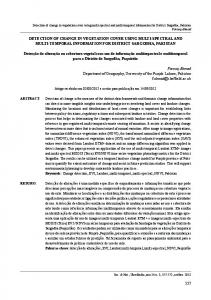
The State of Chiapas is in the southeastern part of Mexico (Figure 1).The physiography of the study area included parts of the Pacific Coastal Plain, Sierra Madre, Central Depression, and Central Plateau. The central and the southwest portions of the image were primarily in the Sierra Madre, while the northeast portion of the study area was in the Central Depression. This region had experienced several deforestation events, mainly due to agriculture activities and forest fires. February

1998 PE&RS

1

Chiapas, Mexim MSS Scene Path 22, Row 49 4017 lines x 4571 samdes

__.II

Figure 1.Chiapas scene, 11March 1986.

Forest harvesting has had a major influence i n the Central Depression area of the State of Chiapas during the 1980s. The images used in this study were three co-registered MSS scenes from the Chiapas area i n the Landsat World Reference System-2, path 22 and row 49. The 1970s image was obtained on 05 December 1975 (Figure 2), the 1980s image was obtained on 11 March 1986 (Figure 3), and the 1990s image was made from a composite of images (Figure 4) obtained on 03 March 1992 a n d 04 April 1992 (Lunetta et al., 1993). A composite was necessary because of cloud cover, and was made according to the procedures used by the EROS Data Center and described i n Lunetta et al. (1993). All images were i n the UTM projection within zone 15. Each pixel was resampled into a 50-metre ground resolution, and the datum used was NAD27. The scene size was 1024 by 1024 pixels. The compilation of the triplicate images and registration were performed by the EROS Data Center (Lunetta et a]., 1993). Several changes were observed directly from the three scenes. They included changes From forest to fire burns. Most of the fire burns existed in the northeastern portion of the 1986 scene, but they also existed in the central and southeast portions of the 1986 scene. From land to reservoir. One new reservoir was constructed in the southeast portion of the 1986 scene. From cloud to land. A typical area of this type of cloud obstruction of land cover was located at the eastern lakeshore in the 1986 scene. From fire burns to vegetation regrowth. This type of change happened in the previous burned areas, and regrowth was found in the 1992 scene. From land to clouds. The majority of this type of change existed in the south-central portion of the 1992 composite, but was also scattered in other parts of the 1992 scene. From water to clouds. A typical place where this type of PE&RS

February 1998

change was found was in the reservoir in the 1992 composite. The data processing procedures for vegetation index change detection consisted of vegetation index transformations, vegetation index differencing, and evaluations of change statistics. The vegetation index transformations were performed using the formulas detailed previously. In the computations, the following modifications were made: The computed vegetation indices were linearly stretched from a given interval (mean - 2 * standard deviations, mean + 2 * standard deviations) to 0, 255. Any VI value that was beyond the mean ? 2 * standard deviations was truncated to these boundary values. This process was used to eliminate any outlier measurements in the data sets, and to convert VIS so that they could be recorded in 8-bit image files. Because of the linear stretching process, DVI and PVI transformations actually produced the same results; RVI and SARVI produced similar results; NDVI, SAVI, and TSAVI also had similar results. The stretched VI values were again "nearly linearly" stretched from 0,255 to 0,1.The "nearly linearly" means mapping 0, 5 to 0 and linearly mapping 6, 255 to 0,1. These scaled vIs were classified into 11 classes. The resulting images were stored in raster GIS files. The vegetation index differences were performed based on the scaled 0 , l images. These differences were again placed into 11 classes according to the values of the difference. The resulting image was also recorded in a raster GIs file. The number of pixels i n each of the 11 change classes was obtained by counting pixels in that class. The percentage of a change class in a scene was obtained by dividing the number of pixels i n the class by 1024 by 1024 or the total number of pixels. The results of these experiments were evaluated i n three

Mexico Chiapas Subscene Band 1, 2, 4 Composile (12105175) Scene Size: 1024x1024; Pixel Size:50x50 m UTh4 Zone IS;UL: N1809000,E469900,LR:N1757800,E521100

I1M ISLPTIle : 7m.m

lar i n terms of spatial distribution pattern and statistical characteristics. Generally speaking, the subtraction-group w s had strong multiple peak distributions. The ratio-group VIs had strongly biased distributions with peaks falling towards the tail of the distribution. The ratio-group VIS had normal-like distributions. It was still unknown whether these phenomena were generalized phenomena or just localized phenomena. However, this fact made NDVI a better transformation for statistical analyses of the study data. All v~ maps identified the water surfaces present i n the study area. The spatial distribution pattern for different VIs within a given group were similar. As far as the degree of greenness of vegetation was concerned, the RVI appeared to be the most sensitive, as it was located i n a large area of I (between 0.9 and 1.0). The NDVI was the least high R ~ values sensitive because it located only a small area of high NDVI values (between 0.9 a n d 1.0). Vegetation Index Images

Figure 2. Landsat M s s subscene, 1975.

For the 1975 vegetation index images, the R ~ group I of vegetation indices was affected strongly by topographic conditions, as evidenced by the SW-NE color trends that followed the topography in the 1975 RVI map. (Color images are produced in black and white here due to cost constraints.) The NDVI was the least affected by local topography. 1986 vegetation index maps all exhibited fire scars which were clearly detected by all v~groups. However, DVI indicated a larger burn in the fire-bum areas. Some burnt areas had DVI values close to zero. For the high VI value class (between 0.9 and 1.0), all three VIS had similar spatial estimations. 1992 vegetation index maps indicated forest regrowth in the I RVI showed more previously fire-burned areas. Again, D ~ and

ways. First, satellite imagery used in the analysis and other satellite scenes were interpreted to evaluate the results of vI groups. Second, local experts from Chiapas, Mexico were involved i n the evaluations of results in the laboratory and in the field. Third, local experts and project personnel traveled to Chiapas to evaluate results i n the field.

Mexico Chiapas Subscene Band 1,2, 4 Composite (03/11186)

Scene S i : 1024x1024; Pixel Size: 50x50 m UTM Zone IS; UL: N1809000,E469900;LR: N1757800,ES21100

Results Some immediate observations could be made based on the scene statistics (Table 2, Figures 5 to 7). The 1986 sub-scene had smaller ranges and a bigger mean, median, and mode for all the four bands as compared to the 1975 scene. These characteristics suggested that the 1986 image had changed significantly due to changes in land cover, and from atmospheric and sensor affects and sun position. Because the darkest and brightest areas should be present in both scenes, they should have the same or similar spectral properties if there were no atmospheric or sensor affects on both dates. It was intuitive that the decreasing range should be mostly due to the atmospheric and sensor affects. Therefore, it was deemed best tostretch the spectral bands of both scenes to similar ranges and then conduct the work, so as to have spectral similarity for both scenes. The 1992 scene was a composite of two dates (Figure 4). Due to the cloud affects, the maximum values for all bands were signific:antly higher than those from the 1975 and 1986 scenes. The band distribution ranges of the 1992 scene were similar to those of the 1986 scene, hut different from those of the 1975 scene. Temporal equalization was necessary in order to reduce the atmospheric and sensor affects. Vegetation index and difference images were constructed for all seven vegetation indices and from all three scenes. Results showed t h i t the vegetation index maps obtained by vI transformations within each computational group were simi146

1@

Figure 3. Landsat MSS subscene, 1986.

February 1998 PE&RS

Mexico Chinpas Subscene Band 1,2,4 Composite (03103192and 04104192composite) Scene Sze: 1024x1024; Pixel Sze:50x50 m UTM Zone 15;UL: N1809000,E469900,LR: N1757800,E521100

-LMWa

=

: 9210.1M 1:503936 I

I

Figure 4. Chiapas scene, 03 March 1992 and 04 April 1992 composite.

burn area and seemed to be more sensitive than NDVI. The cloud covered area over the land usually had VI values between 0.1 to 0.2. These areas should be distinguished from those vegetation regrowth areas. In addition, scattered clouds over the reservoir water significantly affected all vegetation indices.

Discussion Changes between 1986 and 1975 (Figure 5) were primarily from loss of vegetation caused by deforestation and/or forest fires, reservoir construction, and cropping activities. The positive changes in the difference images were represented by green colors, the negative changes were represented by reddish colors, and areas of no change were represented by dark black in the original color composite images. (Again, color images are produced in black and white here due to cost

Direction

Negative

Range

Change Class 1975 -

1986

Change %

1992 1975 -

1992

PE&RS

February 1998

constraints.) All three VI groups clearly identified the land to reservoir change that occurred between 1975 and 1986. Both DVI and RVI difference images were affected by topographic factors. DVI and RVI difference images estimated about 1.5 percent and 1.3 percent net deforestation and loss of vegetation for the whole scene. According to our visual and field interpretations of change, these statistics underestimated the actual change from deforestation. The NDVI difference images located about 6.8 percent net deforestation and loss of vegetation, and this number was more consistent with our visual interpretations from images and from the field evaluations. Changes between 1992 and 1986 (Figure 6) occurred in two manners: the overall deforestation and loss of vegetation in the whole scene, and the vegetation regrowth in previ-

Positive

0

Net Gain

DVI RVI

39.77 37.13

21.93 27.03

38.30 35.84

-1.48 -1.27

insensitive insensitive

(1) Deforestation (2) Forest 4

NDVI

38.12

30.52

31.36

-6.76

acceptable

(3) Land

DVI RVI NDVI DVI RVI NDVI

36.11 29.59 31.69

31.45 37.60 36.97

32.44 32.81 31.34

-3.67 3.22 -0.35

(1) Deforestation (2) Fire Scars +

42.52 38.74 41.77

21.23 24.40 26.37

36.25 36.86 31.86

-6.27 -1.88 -9.91

inconsistent unacceptable acceptable insensitive insensitive acceptable

Comments

Major LandCover Changes

Fire Scars + Water

Vegetation Regrowth (1) Deforestation (2) Land + Water

1986 And 1975 NDVl Difference Map Mexico Chiapas Subscene Scene Size: 1024x1024: Pixel Size: 50x50 m UTM Zone 15; UL: N1809000,E469900,LR: N1757800,a21100 DVI Diff. Value

Points

RVI Diff.

%

Poinla

46

-10 - 9

1216.

0.12

365.

0.03

-

3906.

0.37

1053.

0.10

-8

-7

NDVl Diff. Points

%

Figure 5. 1986 and 1975 RVI difference map.

1992 And 1986 NDVl Difference Map Mexico Chiapas Subscene Scene Sue: 1024x1024; Pixel Size: 50x50 m UTM Zone 15; UL: N1809000,E469900;LR: N1757800,E521100 Palien

u

Value -10

-

9

DVI Diff. 46

Points 1234.

0.12

RVI Diff, Points 947.

96 0.09

NDVl Diff. Points 582.

% 0.06

111

w

II II

m i%lil

111

m H Figure 6. 1992 and 1986 DVI difference map.

February 1998 PE&RS

1992 And 1975 NDVl Difference Map Mexico Chiapas Subscene Scene Size: 1024x1024: Pixel S i :50x50 m UTM Zone 15; UL: N1809000,E469900,LR: N1757800,E521100

SCNZ

P

Paaern

: 9275mDVI.',i.

m m

1:603936

Points

Vdw

NDVl Diff. %

RVI Dim. Pointa %

DVI Diff. ILUP nLQw5

%

Points

-9

1512.

0.14

306.

0.03

4.

0.00

-8

- -7

4171.

0 40

3733.

0.36

1573.

0.15

-6

- -5

21658.

207

22092.

2.11

7-6,

0.72

-4

- -3

11-1-

11.01

6

9.25

,7834.

5.32

-2

- -1

303010-

28.90

262971

26.99

371087.

3S.39

222596.

21.23

255901.

24.40

276462.

26.37

2

ZSl152.

--95

266076.

21.28

2-7

25.39

3 - 4

93646.

8.93

75215.

7.17

5 - 6

26441.

2.52

18252.

1

-10

O

-

-

7

56072.

5.35

9811.

0.94

1633.

0.16

355.

0.03

Figure 7 . 1992 and 1975 NDVI difference map.

ously burned areas. The magnitude and direction of changes were in the same All three vI groups were sensitive to the cloud cover present in the 1992 composite, and indicated those areas as negatively changed areas. The DVI differencing map estimated a 3.7 percent loss in vegetation and forest, which was not consistent with its estimate for the 1975 to 1985 changes. The interpreted change in vegetation cover from 1975 1986 was greater than 1986 to 1992. The RW difference image indicated a 3.2 percent gain in vegetation from 1986 to 1992, and this estimate was unacceptable according to our visual analysis. The loss in vegetation by NDVI differencing was about 0.4 percent, which we believe was the most acceptable number from interpretations of images and field work. The overall changes between 1992 and 1975 (Figure 7) were loss of vegetation caused by deforestation, fire, reservoir construction, and cropping activities. The magnitude and direction of changes were represented in the same way in the difference images. All three v~ groups were sensitive to the cloud cover present in the 1992 composite, and indicated those areas as having experienced negative change. The land-to-reservoir change was identified by all three VI groups. The positive "greenish" colored changes were mainly in the southern part of the scene whereas the negative "reddish" colored changes were mainly concentrated on the northeastern part of the scene. The DVI and RVI difference images provided smaller quantities (6.3 and 1.9 percent, respectively) for estimating the loss of vegetation, which potentially underestimated the vegetation change that had occurred in the last two decades. The NDVI difference image provided a 9.9 percent loss in vegetation, which was more consistent with our visual interpretations, and estimates from local Mexican experts and from field work.

PE&RS

February 1998

Conclu~ion~ The change in the study area between 1975 and 1986 was dominated by deforestation and loss of vegetation resulting from fires, reservoir consttuction, and cropping activities. F~~~ 1986 to 1992, the change was dominated by general loss of vegetation and vegetation regrowth in the previous fire burned areas, ~ ~from NDVI ~ indicated ~ lthat this t re- ~ gion had experienced consistent change in vegetation and deforestation, with an overall rate of change in vegetation land covers of about 10 percent from 1975 to 1992. An interesting trend was that the net rate of change in this region dropped from more than six percent for the 1975 to 1986 period to less than one percent for the 1986 to 1992 period. Several conclusions stemmed from using different vegetation index groups: In the study area, N D ~ Iusually had a normal distribution histogram. RVI usually had a highly skewed, exponential-like histogram distribution. DVI usually had a multiple peak, mixed histogram distribution. All three VI groups were found to clearly distinguish land surfaces, water surfaces, and cloud covers. Therefore, these algorithms can identify changes among these land-cover and cloud types. DVI did not provide consistent change statistics for the change detections conducted in the two successive periods. RVI did not provide acceptable change statistics for the slower rate of vegetation change processes that occurred between 1986 and 1992. Both D ~ and I RVI were more affected by topographic factors than N D and, ~ therefore, potentially produced less useful results than the NDVI method i n this study area.

Acknowledgmenf~ The authors wish to thank a number of people who helped in this work. Our thanks to Dr. Gene Meier and Captain John

Moore of the U.S. Environmental Protection Agency and U.S. Public Health Service, respectively; James Sturdevant a n d T o m Loveland of t h e U.S. Geological Survey; John Dwyer of Hughes STX; a n d Dr. James Lucas of Lockheed Martin.

References Anderson, G., and J. Hanson, 1992. Evaluating hand-held radiometer derived vegetation indices for estimating above ground biomass, Geocarto International, 1:71-77. Angelici, G., N. Brynt, and S. Friendman, 1977. Techniques for land use change detection using Landsat imagery, Proceedings of the American Society of Photogrammetry, Falls Church, Virginia, pp. 217-228. Banner, A., and T. Lynham, 1981. Multitemporal analysis of Landsat data for forest cut over mapping - a trial of two procedures, Proceedings of the 7th Canadian Symposium on Remote Sensing, Winnipeg, Manitoba, Canada, pp. 233-240. Cairns, M., R. Dirzo, and F. Zadroga, 1995. Forests of Mexico, Journal of Forestry, July, pp. 21-24. Derring, D., and R. Haas, 1980. Using Landsat Digital Data for Estimating Green Biomass, NASA Technical Memorandum #80727, 2 1 p.

Eidenshink, J., 1992. The North American Vegetation Index Map, 1: 12,500,000 Scale, U.S. Geological Survey, Reston, Virginia. Eidenshink, J., and R. Haas, 1992. Analyzing vegetation dynamics of land systems with satellite data, Geocarto International, 1:53-61. Elvidge, C., and R. Lyon, 1985. Influence of rock-soil spectral variation on the assessment of green biomass, Remote Sensing of Environment, 17:265-279. Gomarasca, M., P. Brivio, F. Pagnoni, and A. Galli, 1993. One century of land use change in the metropolitan area of Milan (Italy), International Journal of Remote Sensing, 14:211-223. Hochheim, K., and P. Bullock, 1994. Operational estimates of Western Canada spring wheat yield using NOAAIAVHRR LAC data, Proceedings of the 12th Pecora Symposium, ASPRS, Bethesda, Maryland, pp. 143-150. Huete, A., and C. Tucker, 1991. Investigation of soil influences in AVHRR red and near-infrared vegetation index imagery, International Journal of Remote Sensing, 12:1223-1242. Jackson, R., P. Slater, and P. Printer, 1983. Discrimination of growth and water stress in wheat by various vegetation indices through clear and turbid atmospheres, Remote Sensing of Environment, 13:187-208. Jensen, J., 1996. Introductory Digital Image Processing, Prentice-Hall, Englewood Cliffs, New Jersey, 316 p. Justice, C., J. Townshend, and B. Choudhury, 1989. Comparison of AVHRR data for monitoring vegetation phenology on a continental scale, International Journal of Remote Sensing, 10:1607-1632. Lillesand, T., and R. Kiefer, 1987. Remote Sensing and Image Interpretation, John Wiley and Sons, New York, New York, 721 p. Loveland, T., J. Merchant, D. Ohlen, and J. Brown, 1991. Development of a land-cover characteristics database for the conterminous United States, Photogrammetric Engineering b Remote Sensing, 57:1453-1463. Lunetta, R., J. Lyon, J. Sturdevant, J. Dwyer, C. Elvidge, D. Yuan, L. Fenstermaker, S. Hoffer, and R. Weerackroon, 1993. North American Landscape Characterization (NALC-Pathfinder) Project Research Plan, U.S. Environmental Protection Agency report EPA/600/R-931135, 427 p. Lyon, J., and L. George, 1979. Mapping vegetation communities in

the Gates of Arctic National Park, Alaska, Proceedings of the Annual Convention of the American Society for Photogrammetry, Falls Church, Virginia, pp. 483-497. Lyon, J., and J. McCarthy, 1995. Wetland and Environmental Applications of GIs, CRCJLewis Publishers, Boca Raton, Florida, 373 P. Marsh, S., J. Walsh, C. Lee, L. Beck, and C. Hutchinson, 1992. Comparison of multi-temporal NOAA-AVHRR and SPOT-XS satellite data for mapping land-cover dynamics in the west African Sahel, International Journal of Remote Sensing, 13:2997-3016. Nelson, R., 1983. Detecting forest canopy change due to insect activity using Landsat MSS, Photogrammetric Engineering b Remote Sensing, 49:1303-1314. Paloscia, S., and P. Pampaloni, 1992. Microwave vegetation indexes for detecting biomass and water conditions of agricultural crops, Remote Sensing of Environment, 40:15-26. Perry, C., and L. Lautenschlager, 1984. Functional equivalence of spectral vegetation indices, Remote Sensing of Environment, 14: 169-182. Price, J., 1992. Estimating vegetation amount from visible and near infrared reflectances, Remote Sensing of Environment, 41:29-34. Qi, J., A Huete, M. Moran, A. Chehbouni, and R. Jackson, 1993. Interpretation of vegetation indices derived from multi-temporal SPOT images, Remote Sensing of Environment, 44:89-101. Ray, T., T. Farr, and J. Van Zyl, 1993. Proceedings of Tropical Symposium on Combined Optical-Microwave Earth and Atmosphere Sensing, Albuquerque, New Mexico. Richardson, A,, and J. Everitt, 1992. Using spectral vegetation indices to estimate rangeland productivity, Geocarto International, 1:63-77. Short, N., 1982. The Landsat Tutorial Workbook: Basics of Satellite Remote Sensing, National Aeronautics and Space Administration Reference Publication 1078, Washington, D.C. Singh, A., 1989. Digital change detection techniques using remotelysensed data, International Journal of Remote Sensing, 10:9891003. Tappan, G., D. Tyler, M. Wehde, and D. Moore, 1992. Monitoring rangeland dynamics in senegal with Advanced Very High Resolution Radiometer data, Geocarto International, 1:87-98. Thenkabail, P., A. Ward, L. Lyon, and C. Merry, 1994. Thematic Mapper vegetation indices for determining soybean and corn growth parameters, Photogrammetric Engineering 6.Remote Sensing, 60:437442. Tucker, C., 1979. Red and photographic infrared linear combination for monitoring vegetation, Remote Sensing of Environment, 8: 127-150. Turcotte, K., W. Kramber, G. Venugopal, and K. Lulla, 1989. Analysis of region-scale vegetation dynamics of Mexico using stratified AVHRR NDVI data, Proceedings of the Annual Convention of the American Society for Photogrammetry and Remote Sensing, Baltimore, Maryland, 3246-257. Vanderventer, P., A. Ward, P. Gowda, and J. Lyon, 1997. Using Thematic Mapper data to identify contrasting soil plains and tillage practices, Photogrammetric Engineering 6.Remote Sensing, 63: 87-93. Van Leeuwen, W., A. Huete, A. Begue, J. Duncan, J. Franklin, N. Hanan, S. Prince, and J. Roujean, 1994. Evaluation of vegetation indices for retrieval of soil and vegetation parameters at HapexSahel, Proceedings of the 12th Pecora Symposium, ASPRS, Bethesda, Maryland, pp. 188-197. (Received 19 June 1996; accepted 5 November 1996; revised 28 April 1997).

February 1998 PE&RS