509. A Class of Nonlinear Filtering Problems. Arising from Drifting Sensor Gains. Tyrone L. Vincent, Member, IEEE, and Pramod P. Khargonekar, Fellow, IEEE.
IEEE TRANSACTIONS ON AUTOMATIC CONTROL, VOL. 44, NO. 3, MARCH 1999
509
A Class of Nonlinear Filtering Problems Arising from Drifting Sensor Gains Tyrone L. Vincent, Member, IEEE, and Pramod P. Khargonekar, Fellow, IEEE Abstract— This paper considers a state estimation problem where the nominal system is linear but the sensor has a timevarying gain component, giving rise to a bilinear output equation. This is a general sensor self-calibration problem and is of particular interest in the problem of estimating wafer thickness and etch rate during semiconductor manufacturing using reflectometry. We explore the use of a least squares estimate for this nonlinear estimation problem and give several approximate recursive algorithms for practical realization. Stability results for these algorithms are also given. Simulation results compare the new algorithms with the Extended Kalman Filter (EKF) and Iterated Kalman Filter (IKF).
where
and and are matrices of appropriate dimensions. We to be an unknown process disturbance, to will consider be a known input, and to be measurement noise. The matrix is a time-varying diagonal matrix which represents the variation in the gain of each sensor. Although many models are possible, we will assume for the dynamic behavior of the following: (3) (4)
Index Terms— Calibration, estimation, nonlinear systems, observers.
I. INTRODUCTION AND PROBLEM FORMULATION
T
HE MAIN goal of this paper is to study a particular nonlinear estimation problem arising from drifting sensor gains. A practical example of this problem occurred in our work on control and estimation in semiconductor manufacturing [1]. In plasma etching and deposition processes, a laser is reflected off the wafer while it is undergoing processing. The wafer consists of a stack of thin films on a substrate. As the wafer is processed, the reflected light intensity varies as a function of the film thickness. Thus, current thickness and etch (or deposition) rate information can be recovered from this time-varying signal which is recorded using analog and digital electronics. However, this signal is also affected by factors other than the changes in the film thickness. In particular, an important source of signal variation is the gradual clouding of the optical window through which the laser and detector view the wafer. This clouding occurs because of polymer formation in the plasma which diffuses and sticks to the windows on the reactor and decreases the effective gain of the system during the etch process. There are other sources of variations as well, such as drifts in the analog electronics, variations in the optical system, etc. To account for this variation, one can postulate a model for the sensor drift. Consider the following discrete-time system: (1) (2) Manuscript received July 8, 1997; revised April 4, 1998 and May 1, 1998. Recommended by Associate Editor, J. C. Spall. This work was supported in part by the AFOSR/ARPA MURI Center under Grant F49620-95-1-0524. T. L. Vincent is with the Engineering Division, Colorado School of Mines, Golden, CO 80401 USA. P. P. Khargonekar is with the Electrical Engineering and Computer Science Department, University of Michigan, Ann Arbor, MI 48109 USA. Publisher Item Identifier S 0018-9286(99)02129-7.
and and are matrices of where appropriate dimensions. We will assume throughout that and are invertible. By choosing we assume that the gain perturbations are additive around a nominal value of one, while the dynamics allow us to specify a Note a choice general (finite-dimensional) spectrum for and such that and allows the of trajectory of the sensor drift to be independent of the state The system formulation emphasizes the conception of as a known, nominal gain for the system, and as a time-varying perturbation of this gain. The goal is to obtain online estimates of and using This is a filtering problem where the main difficulties arise from the nonlinear output equation. The mathematical estimation problem described above in (1)–(4) captures a class of sensor signal processing problems where the sensor gain drift has a systematic component. We believe that such problems also arise in applications other than the film thickness and etch rate estimation problem discussed above. For example, online sensor self-calibration problems will also lead to estimation problems of the kind treated in this paper. From a system theoretic viewpoint, this is a special class of nonlinear filtering problems. The standard approach [2] is to calculate the a posteriori conditional probability density of and which is conditioned This on the observed output sequence distribution contains all the statistical information we have and given our observations. Estimates of about and are then generated by operating on the a posteriori density. For example, the minimum variance estimate of and would be given by the conditional mean [2], [3]. Another common estimate, termed maximum a posteriori (MAP) [4], [5], or Bayesian Maximum Likelihood [2] is given which can be thought of by finding the maximum of as the state and gain perturbation which was “most likely”
0018–9286/99$10.00 1999 IEEE
510
IEEE TRANSACTIONS ON AUTOMATIC CONTROL, VOL. 44, NO. 3, MARCH 1999
given the observed output sequence. Unfortunately, when the dynamics and/or the output equations are nonlinear, calculation becomes nontrivial and essentially intractable as an of engineering solution. The main goal of this paper, besides exposing this very structured and interesting class of nonlinear filtering problems, is to exploit this special structure and explore suboptimal but more easily computable estimates. Here we will consider a family of estimation procedures which are all based on a least squares approach. The analysis begins with the case in which is an unknown constant, i.e., Here we show that there is a nonzero bias in the estimate which can be taken care of if it is known a priori that is an unknown constant. Next we give an asymptotic convergence result under the assumption of zero noise. Following this, we present a general scheme for computing the estimates. We then show various approximations which lead to the extended Kalman filter and iterated Kalman filter as special cases and also lead to other new estimators. Stability results for these new estimators are given. Finally, a simple numerical simulation is included to illustrate the ideas. This filtering problem has a considerable amount of structure and we are currently exploring additional properties and different estimation schemes.
are chosen, are fixed by the system equations (5) and (6); however to be explicit, on we notate here and elsewhere the dependence of We will also use separate notation for estimated and actual trajectories in the following way: The true trajectory will be while an estimated trajectory will denoted by a star, e.g., with the added annotation of use a hat notation, e.g., to indicate the estimate of the state at time given data up to time Let us define (7) (8) and define an abbreviation for the output equation
Furthermore, we will notate sequences from time or if the initial time is zero, by we may rewrite our cost function as
to
as Then
A. Notation denote the vector space -tuples of real numbers. Let where We will often use the quadratic form and is a symmetric positive definite matrix. For ease of notation, we will use the norm and dot product notation and with if The ) indicates a matrix with the elements of vector notation along the diagonal and zeros elsewhere. The maximum and the minimum singular value of a matrix is notated We define a neighborhood singular value is denoted by
II. LEAST SQUARES ESTIMATE The suboptimal approach we will investigate for the estiin the face of a drifting gain is based mation of state on least squares optimization. We will consider estimation via minimization of the quadratic cost function
subject to the constraints (5) (6) and are a priori guesses for the initial condition Both and of the system. Now, it is clear that once
(9) subject to the constraint (10) Consider the minimizing solution of (9) This will correspond to the state trajectory which can be explained by noise and disturbances which are the and smallest in the sense of the norms This type of curve-fitting approach makes intuitive engineering sense, and the least squares approach to nonlinear filtering problems has a long history [6]. This approach is in the same vein as other work in nonlinear observers, specifically moving horizon observers [7] and Newton observers [8]. Moving horizon observers approximately solve a moving horizon optimization problem, with the accuracy increasing with time. Newton observers use a Newton algorithm to invert the dynamics given output data, which is also equivalent to approximately solving a moving horizon optimization problem. If we make some particular probabilistic assumptions about our disturbances and noise, it is well known that the least squares estimate is related to a type of maximum likelihood (ML) estimate. In this case, we will be considering the which is the distribution of the joint density conditioned on the observations The entire trajectory of (9) corresponds to the Bayesian minimizing solution if Maximum Likelihood estimate maximizing we assume Gaussian noise, disturbance, and initial state distributions. The exact relationship is given in the following theorem, which follows directly from [9] and [2].
VINCENT AND KHARGONEKAR: CLASS OF NONLINEAR FILTERING PROBLEMS
Theorem 1: Consider the system (1)–(3) with random initial and state and gain densities and white Gaussian noise and disturbance random sequences and Let the initial state, noise, and disturbance be mutually independent. Then the cost function (9) is proportional to the negative log of the joint a posteriori distribution Since the maximum likelihood estimate is given by maximizing the joint a posteriori distribution, the minimizing solution of (9) will correspond to the maximum likelihood estimate. Because of this connection, we will term the minimizing the joint maximum likelihood (JML) estimate. solution It should be emphasized, however, that the JML estimate rather than the seeks to find the “most likely” trajectory which would be given by maximizing “most likely” state In particular, because of our nonlinear output lies on (that is, equation, there is no guarantee that ) However, for linear dynamics and output that equation, with Gaussian noise and disturbance, it is in fact and this also coincides with the known that minimum variance estimate [2]. a new optimization problem must be solved To find each time a new data point is collected, and the number of parameters increases with the number of observations. Obviously, we will quickly lose the computational advantage we were seeking over the minimum variance estimate. Therefore, we will be interested in ways of reducing the complexity so that the computation time does not grow with the number of data points. III. SPECIAL CASE:
511
Proof: As stated above, for fixed , the JML estimate coincides with the minimum variance estimate. The minimum cost given as a sum of the weighted residuals as in (11) can be obtained using orthogonal transformations [10, Ch. 7]. For a direct algebraic proof, see [11]. is given by Thus we see that the JML cost for fixed the difference between a Kalman filter prediction designed for the given and the observed output. The JML estimate is then possible by adjusting to minimize this error. This class of algorithms for parameter estimation, known as prediction error (PE), has been studied extensively, both in the offline and recursive cases; see for example [12]–[14] and the references therein. we might hope that the estimate given As that by minimizing (11) converge to the actual value of to be consistent. However, this is not is, we would like the case. Consider a (nonjoint) ML estimate of given by Note that maximizing the a posteriori distribution via we can obtain this distribution from
Under the assumptions of Theorem 1, with the exception of considering an unknown constant, we have [15]
UNKNOWN CONSTANT
We can gain insight into the properties of the JML estimate by considering the special case where becomes an unknown constant. Now the problem is essentially one of parameter estimation. Let us consider the We can isolate this part of the JML estimate of for each estimation problem by considering the cost function
(12) and where again, and are the Kalman Filter mean and covariance time updates for fixed Since log is a monotonic function, we can Those terms maximize (12) by minimizing which are dependent on are as follows: of (13)
For fixed since the problem becomes linear, the JML and (and ) coincide minimum variance estimates of is related and are given by a Kalman filter. The cost to the output of a Kalman filter designed for a fixed via the following result. For ease of notation, we define Theorem 2: Consider the JML cost (9) subject to constraint and Then (10) with is given by (11) and and are the Kalman filter mean and covariance time updates for fixed
where
The estimate of obtained by minimizing (13) is known to be consistent with probability one [15]. A key difference between and because this term (11) and (13) is the term is lacking, we lose the property of consistency. This problem can obviously be alleviated by the inclusion in (11) of this extra term. However, in the general case, with time-varying analysis of the estimator bias is very difficult, and a similar fix cannot be accommodated. IV. RESULTS
IN THE
GENERAL CASE
We have seen in the previous section that for a special case of constant , we cannot expect consistent estimates. However, if we are content to concern ourselves only with the stability of the estimates, it is possible to show that the estimated trajectories approach the actual trajectories in the noiseless
512
IEEE TRANSACTIONS ON AUTOMATIC CONTROL, VOL. 44, NO. 3, MARCH 1999
case. That is, we assume that the data generated by the system
has been (14) (15)
Note that in this analysis we are not limited to the special case of constant. To consider the stability of the JML estimates, we need to introduce a notion of observability. Let and Consider the mapping
Let
Clearly
for all
satisfying the constraints (10). Thus
where similarly for
indicates it is the Let
th member of
and
then by induction given by where is the output and input of system (14) and (15) for initial condition We will say that the and if system is -observable with respect to is injective for all Basically, what we require is, the state at time zero given the input for time should be uniquely defined by the observed output sequence. There is another notion of observability which will be more useful for the recursive algorithms which are described later. at is the system is said to satisfy If the rank of [16]. By the rank observability condition at for input the chain rule, we have
Now, let Then
be the state trajectory of the nominal system.
for all Since we must necessarily have
minimizes the cost function,
Therefore .. .
(16) for all
where
Thus the system satisfies the rank observability condition at for if the matrix is of rank This matrix will be called the observability matrix. Theorem 3: Consider system (14) and (15) with initial conresulting in the state trajectory dition and input Consider estimation of via minimization of be positive definite. If (9) subject to constraint (10). Let system (14), (15) is -observable with respect to and and then as Proof: The idea is to bound the cost function using the actual output of the deterministic system and then note that each element of the cost function is nondecreasing with . Thus the minimum value of the cost function must converge to the value given by the true solution as time goes to infinity, and by continuity and observability, the estimated state must converge to the true state. to indicate the value We will use the notation of the cost function used at time given by plugging in the and ( will, of course, have first components of to be greater than .) Then
which implies This implies
and
as
Since we have assumed by -observability that uniquely defines and because the mapping to output sequence is continuous, we have that from state as Weaker conditions on the input, state, and estimate trajectories are possible, but the essence of the proof is the same. V. APPROXIMATIONS AND RECURSIVE ALGORITHMS The general solution of the JML estimate requires solving a nontrivial constrained least squares problem with the number of parameters increasing with time. Usually, given data at time we are most interested in finding which is the th term Let of the most likely trajectory
Clearly Using a dynamic programming in a recursive approach, it is possible to construct manner [9]:
(17)
VINCENT AND KHARGONEKAR: CLASS OF NONLINEAR FILTERING PROBLEMS
Thus, it is possible to reduce the parameter space to the If the output equation were linear, then it is dimension of is a purely quadratic function for all well known that and it is possible recursively compute the “sufficient statistic” of the center and Hessian of the quadratic. Unfortunately, for in our case a finite-dimensional representation of all is not possible. However, a possible solution technique with a which will be explored here is to approximate function of fixed structure. We are aided in our search for an due to the nature of the estimation online approximation of problem (as opposed to a control problem), as we will have on hand some estimates of the past true trajectory, and this is the region where the approximation must be good. Historically, recursive approximate solutions to the nonlinear least squares problem have been developed using linearization of the dynamics and output equation [9], or the technique of invariant imbedding [6], which give rise to equations equivalent to or very similar to the extended Kalman filter (EKF). We shall see below how the EKF is related to the technique of approximation of We will consider the following types of algorithms: • strictly recursive approximations: A fixed parameterized is postulated, and at each parameters structure for are computed; to approximate the cost function • partially recursive approximations: As described below, in a manner similar to windowing, more data is used to compute the estimates, so that at time we need only for some find an approximation of A. Strictly Recursive Approximations We begin by considering a strictly recursive approximation. A possible scheme for solving (17) is as follows. Algorithm SR Given initial estiwhere
Step SR0: For initialization: set and weight let mate and Step SR1: Set
513
Step SR3: Approximate
by
for some choice of and Step SR4: Go to Step SR1. Note: in Step SR3, the approximation should strictly speakwith a ing be given by constant. However, because will only be used later to define a minimization problem, this constant is unimportant. The same reasoning allows us to disregard the constant term in is Step SR1. We see that, under the assumption that quadratic, Step SR1 is exact. The approximate nature of the algorithm comes from Steps SR2 and SR3. Because the function to be minimized in Step SR2 contains quartic terms due to our nonlinear output equation, minimization requires the use of a gradient descent-type algorithm. Errors may occur by converging to a local minimum or stopping the algorithm before convergence occurs. Efficient algorithms for the minimization in Step SR2 are the subject of current research. which In Step SR3, we require the approximation of contains quartic terms, by a quadratic. To reduce the errors of this approximation must be good near future estimates that is, where would lie for the exact JML solution. Below, we show how the EKF and Iterated Kalman Filter (IKF) can be viewed as strictly recursive approximations to the JML estimate, followed by some further possible approximate solutions. 1) EKF/IKF as a Strictly Recursive Approximation: The EKF and IKF are usually introduced as approximations to the minimum variance estimate [2], [3]. However, in [17], it is established that the IKF generates the same iterates as a Gauss–Newton method for the minimization problem
Thus, they can also be shown to be strictly recursive approximations to the JML estimate in the form of Algorithm SR. Algorithm EKF
Solve
Step EKF0: It is the same as SR0. Step EFK1: It is the same as SR1. Step EKF2: Approximately solve Since both and be done analytically, and
are quadratic, this can will be quadratic, that is where
where
by taking Gauss–Newton steps, where for the IKF. and by Step EKF3: Approximate and a constant, is unimportant. Step SR2: Solve
for the EKF,
where (18) and
where (19)
514
IEEE TRANSACTIONS ON AUTOMATIC CONTROL, VOL. 44, NO. 3, MARCH 1999
Step EFK4: Go to Step EFK1. Examining this algorithm, we note two areas of concern. First, using a Gauss–Newton method to solve a quartic problem may not be efficient, and indeed could diverge. Also, the approximation in Step EKF3 (which is a second-order with a Gauss–Newton approximation of the expansion of Hessian) may be improved. 2) Taylor Series: Inspired by the EKF/IKF solution, we attempt to improve the estimates by choosing a gradient descent algorithm in Step SR2 with better convergence properties Since appropriate and choosing a better approximation of algorithms are still an area of current research, we will assume that we can solve Step SR2 to obtain a minimizing solution. is a minimum of then the gradient is zero and we If can use a second-order Taylor series approximation. Then we have the following algorithm.
Step PR-T1: Set
Since both
Solve
and
are quadratic, we have
where
Step PR-T2: Solve
subject to
Algorithm SR-T Step SR-T0: Step SR-T1: Step SR-T2: Step SR-T3:
where
It is the same as SR0. It is the same as SR1. It is the same as SR2. by Approximate
is the Hessian of
where
at
In our case (20)
where the
where
is defined in (19), and element given by
is the
element of
is a
matrix with where
and
Step SR-T4: Go to Step SR-T1. Comparing (20) with (18), we see that the EKF/IKF ignores just as a Gauss–Newton method the term involving would in its estimate of the Hessian. If is a unique minimum then the Hessian is positive definite. B. Partially Recursive Approximations With some added computational complexity, we can reduce This is accomplished the effect of our approximations of by including more of the exact least squares terms in Step 3 and pushing the approximate terms into the past. Consider the following algorithm, with an integer is greater than 1. Algorithm PR-T Step PR-T0: For initialization: Set and weight let estimate where
and
Denote the minimizing solution as Step PR-T3: Approximate by
Given initial
with and as defined in Section V-A2. Step PR-T4: Go to Step PR-T1. is approximated by a Note that in Step PR-T3, However, since second-order Taylor series around is not a minimizer of in general, we need to the minimum of in order to put it calculate into the proper form. C. The Stability of Recursive Approximations Since the recursive algorithms are approximate solutions to the JML estimator, they do not share its guarantee of stability. However, the discrete-time EKF has been shown to be locally stable under general conditions [18]–[20], and it is not surprising that similar results for the algorithms presented here can be established. We will use the following general result which applies to estimation algorithms which utilize a minimization step to incorporate observation data.
VINCENT AND KHARGONEKAR: CLASS OF NONLINEAR FILTERING PROBLEMS
515
from C2–C4. Finally, Condition C5 implies for each observability matrix
Theorem 4: Consider the estimation algorithm
the
(21) (22)
(23) (24) Suppose the following assumptions are satisfied. is A1: The function
where and A2: is invertible. A3: There exist A4: A5: There exist . Then there exists
uniformly in
which along with implies Condition A5. Note: Conditions C3 and C4 are assured by algorithm SR-T The update is for a sufficiently large choice of
such that such and
C4:
that such that if
Since and as a choice of positive definite and sufficiently large will ensure that the difference between
and
will not cause Condition C4 to be violated. In addition, we will have
where
C5: The system satisfies the rank observability condition for input for some along the trajectory
Proof: In this case, A1 is satisfied with terms satisfy and boundedness of
which along with the compactness of is of rank implies for some or
and
Proof: See Appendix A. To establish stability of our recursive algorithms, we need only check if conditions A1–A5 are satisfied. Theorem 5: Consider the estimation algorithm SR-T operating on data generated by the system (14), (15) with and input Let the following initial condition assumptions hold. is such that evolves in a compact set C1: C2: and are invertible, and C3: There exist such that
Then there exists
(25)
.. .
operating on data generated by the system
and
such that if
Condition The higher order uniformly in by the Conditions A2–A4 follow directly
for some This, along with the observability condition C5, allows us to conclude via Lemma 6 (see Appendix A) that Condition C3 is satisfied. A similar result can be obtained for algorithm PR-T; see [11] for details.
VI. SIMULATION RESULTS
AND
DISCUSSION
In order to get an estimate of the performance of the PR-T and SR-T algorithms in the face of measurement noise and disturbances, a series of MATLAB simulation experiments were performed. A fifth-order system with three outputs was dynamics were chosen used for all simulations. The state randomly, although stable. The dynamics which model the were chosen to be integrators so drift of the senor gain that the sensor gain drift was a realization of a random walk.
516
IEEE TRANSACTIONS ON AUTOMATIC CONTROL, VOL. 44, NO. 3, MARCH 1999
The resulting system was as follows:
Fig. 1. Typical response for output, state, and sensor gain drift. TABLE I STATE ESTIMATION ERROR WITH INCREASING INITIAL CONDITION COVARIANCE
We compared the EKF, the IKF, with the SR-T algorithm, and the PR-T algorithm with with simulated Gaussian noise and disturbances and, We set for various choices of and with mean initial conditions The input was a square wave of amplitude one and a period of 20 samples. Unless otherwise stated, the values of the parameters were chosen to be while and Each and run was 100 samples long. Typical responses for are shown in Fig. 1. To determine the average performance of each estimator for a given set of parameters, the average rms estimation error was found over 100 different runs, each with a different realization for state disturbance, measurement noise, and initial conditions. The first set of simulations examined the effect of uncerwas varied from tainty in the initial conditions. In this case, .1 to 100, and was varied from .01 to 3. All other parameters were kept at the nominal values described above. The results are shown in Table I. The key effect which is evident is the advantage of the larger number of measurements used by PRT in its measurement update. Even as the initial condition uncertainty increases, it is able to converge quickly, and this is reflected in the smaller errors. Based on this simulation, there appears to be no advantage to using the SR-T algorithm over the IKF. In the next simulation series, we examined the effect of was varied from .1 to 100. The measurement noise, and
TABLE II STATE ESTIMATION ERROR WITH INCREASING MEASUREMENT NOISE
results are given in Table II. Note in this case that the PRT algorithm is the best for smaller measurement noise, but as the noise level increases, this advantage decreases until all algorithms perform similarly. A similar trend can be observed as the state disturbance is increased. For the results in Table III, the state disturbance was varied between .0001 and .1. Notice again that the advantage of the PR-T algorithm is lost for larger disturbances, and curiously the EKF becomes the best choice for large state disturbances. Based on these simulations, it appears that there is an advantage to an approximate least squares algorithm such as PR-T when there is large uncertainty in the initial conditions, but in the face of large persistent disturbances or measurement noise, this advantage is lost. It seems to us that this is most likely due to a broadening of the a posteriori distribution as
VINCENT AND KHARGONEKAR: CLASS OF NONLINEAR FILTERING PROBLEMS
517
and
TABLE III STATE ESTIMATION ERROR WITH INCREASING STAGE DISTURBANCE
hold for all
the noise terms are increased, and the choice of the maximum of this distribution becomes farther away from the optimal. VII. CONCLUSION In this paper we have explored the nonlinear filtering problem posed by a linear system with a drifting sensor gain. This nonlinear filtering problem appears to be very challenging. We have investigated an estimation procedure based on least squares optimization, the JML estimate, which is the maximum likelihood trajectory estimate under Gaussian assumptions. Several approximate recursive algorithms for calculating the JML estimate, SR-T, and PR-T were proposed, based on finding approximations to the least squares estimation cost with a fixed quadratic structure. The connections with these methods to the EKF and IKF were exposed, and stability properties for the SR-T and PR-T estimation schemes were established. Finally, some simulation results were given demonstrating the behavior of the various algorithms. We have seen that when there is large initial condition uncertainty, there seems an advantage to using PR-T algorithm. However, when measurement noise and state disturbances are increased, the performance gain is not as clear. The precise tradeoffs depend on the level of noise and disturbances and error in initial conditions. APPENDIX
Proof: See [21] and [22]. ; Strictly speaking, the result is proven only for however since the recursion is continuous, we can extend the result to Next, the following lemma places a rough bound on the estimation error. Lemma 7: Consider the estimation update (21)–(22) operating on data generated by system (23) and (24). If Assumptions A1 and A3 are satisfied, then
Proof: Let
Then since
Since
is a minimizer of
and
Thus
The stability result of Theorem 4 is established using several preliminary results. We begin by stating a result of Deyst and Price [21], [22], which bounds the covariance matrix of the Kalman filter as long as controllability and observability conditions are satisfied. This result is useful both to show how Condition C3 of Theorem 5 can be satisfied and as a technical result in the sequel. Lemma 6: Consider the following recursion for
with there exists such that
then
and and finite
If
(26) and
Now, we can show that the error after each step as measured is bounded. by Lemma 8: Consider the estimation update (21) and (22) operating on data generated by system (23) and (24). If Assumptions A1–A4 are satisfied, then
where
uniformly in
518
IEEE TRANSACTIONS ON AUTOMATIC CONTROL, VOL. 44, NO. 3, MARCH 1999
Proof: Since
is a minimizer of (21), this implies
After multiplying on the right by we have
Lemma 9: Consider the estimation update (21) and (22) operating on data generated by system (23) and (24). If Assumptions A1–A5 are satisfied, then there exists such that
and using A1,
where Proof: Let
uniformly in and
and
Then
Normalizing, rearranging, and rewriting using norm and dot product notation results in By Lemma 8 which implies
(27) Now
(28) To bound the summation from below, let us pose the following to optimization problem: Choose minimize
Using (27) we have subject to with given. Using standard quadratic optimal control theory, the solution is given by and finally where
where we have also replaced with using the result of Lemma 7. We now need to account for the “time update.” This follows from
where the inequality comes from inverting both sides of Thus condition A4 to give
as desired. In most cases, is not strictly positive definite, so more work is needed to obtain a stability result.
is calculated from the backward recursive relation
with
(see [23, p. 46]). Thus
Lemma 6 supplies the following bound for
:
where Condition A5. Thus
is defined in
and
(29)
VINCENT AND KHARGONEKAR: CLASS OF NONLINEAR FILTERING PROBLEMS
with have
Using (29) in (28), we
519
We can continue this for
to give
Since the first term on the right is nonnegative
Since by Lemma 8, (where we ignore terms which make the right-hand side such that smaller), it is clear that there exists
By our choice of we also have the argument can be repeated for larger with
uniformly in we have
so with
Thus, and we have
Also, (33)
or
Thus
For some as desired. We are now in a position to prove Theorem 4. such that Proof of Theorem 4: By Lemma 9,
and
Since is invertible, we also have for
some
REFERENCES Choose where
and
such that are defined in Condition A3. Now, since as uniformly in there exists
such that and Thus if
(30) Let then for
for
By Lemma 7, if , Thus we also have
(31) Using (31) in (30), we have
(32)
[1] T. L. Vincent, P. P. Khargonekar, and F. L. Terry, Jr., “An extended Kalman filtering based method of processing reflectometry data for fast in situ etch rate measurements,” IEEE Trans. Semiconduct. Manuf., vol. 10, pp. 42–51, 1997. [2] A. H. Jazwinski, Stochastic Processes and Filtering Theory. New York: Academic, 1970. [3] A. Gelb, Ed., Applied Optimal Estimation. Cambridge, MA: MIT Press, 1974. [4] H. L. Van Trees, Detection, Estimation, and Modulation Theory. New York: Wiley, 1968. [5] H. Stark and J. W. Woods, Probability, Random Processes, and Estimation Theory for Engineers. Englewood Cliffs, NJ: Prentice-Hall, 1986. [6] A. P. Sage, Optimum Systems Control. Englewood Cliffs, NJ: PrenticeHall, 1968. [7] H. Michalska and D. Q. Mayne, “Moving horizon observers and observer-based control,” IEEE Trans. Automat. Contr., vol. 40, pp. 995–1006, June 1995. [8] P. E. Morall and J. W. Grizzle, “Observer design for nonlinear systems with discrete-time measurements,” IEEE Trans. Automat. Contr., vol. 40, pp. 395–404, Mar. 1995. [9] H. Cox, “On the estimation of state variables and parameters for noisy dynamic systems,” IEEE Trans. Automat. Contr., vol. 9, pp. 5–12, 1964. [10] G. J. Bierman, Factorization Methods for Discrete Sequential Estimation. New York: Academic, 1977. [11] T. L. Vincent, “Nonlinear estimation with applications to in situ etch rate and film thickness measurements in reactive ion etching,” Ph.D. dissertation, Univ. Michigan, Ann Arbor, MI, Nov. 1997. [12] L. Ljung, System Identification—Theory for the User. Englewood Cliffs, NJ: PTR Prentice-Hall, 1987. [13] T. S¨oderstr¨om and P. Stoica, System Identification. Englewood Cliffs, NJ: Prentice-Hall, 1989. [14] L. Ljung and T. S¨oderstr¨om, Theory and Practice of Recursive Identification. London, U.K.: MIT Press, 1983. [15] J. Rissanen and P. E. Caines, “The strong consistency of maximum likelihood estimators for ARMA processes,” Ann. Statistics, vol. 7, no. 2, pp. 297–315, 1979.
520
IEEE TRANSACTIONS ON AUTOMATIC CONTROL, VOL. 44, NO. 3, MARCH 1999
[16] H. Nijmeijer, “Observibility of autonomous discrete time nonlinear systems: A geometric approach,” Int. J. Contr., vol. 36, no. 5, pp. 867–874, 1982. [17] B. M. Bell and F. W. Cathey, “The iterated Kalman filter update as a Gauss-Newton method,” IEEE Trans. Automat. Contr., vol. 38, pp. 294–297, 1993. [18] M. Boutayeb, H. Rafaralahy, and M. Darouach, “Convergance analysis of the Extended Kalman Filter used as an observer for nonlinear deterministic discrete-time systems,” IEEE Trans. Automat. Contr., vol. 42, pp. 581–586, 1997. [19] Y. Song and J. W. Grizzle, “The extended Kalman filter as a local asymptotic observer for nonlinear discrete-time systems,” J. Math. Systems Estim. Contr., vol. 5, no. 1, pp. 59–78, 1995. [20] B. F. La Scala, R. R. Bitmead, and M. R. James, “Conditions for stability for the Extended Kalman Filter and their application to the frequency tracking problem,” Math. Contr., Signals, Syst., vol. 8, no. 1, pp. 1–26, 1995. [21] J. J. Deyst, Jr. and C. F. Price, “Conditions for asymptotic stability of the discrete minimum-variance linear estimator,” IEEE Trans. Automat. Contr., vol. 13, pp. 702–705, 1968. [22] J. J. Deyst, Jr., “Correction to Conditions for asymptotic stability of the discrete minimum-variance linear estimator,’ ” IEEE Trans. Automat. Contr., vol. 18, pp. 562–563, 1973. [23] A. E. Bryson, Jr. and Y.-C. Ho, Applied Optimal Control. Cambridge, U.K.: Hemisphere, 1975.
Tyrone L. Vincent (S’87–M’91) received the B.S. degree in electrical engineering from the University of Arizona, Tucson, in 1992 and the M.S. and Ph.D. degrees in electrical engineering from the University of Michigan, Ann Arbor, in 1994 and 1997, respectively. He is currently an Assistant Professor at the Colorado School of Mines. His research interests include nonlinear estimation, system identification, and fault detection with applications in materials processing and power systems.
Pramod P. Khargonekar (S’81–M’81–SM’90– F’93) received the B.Tech. degree in electrical engineering from the Indian Institute of Technology, Bombay, in 1977 and the M.S. degree in mathematics and the Ph.D. degree in electrical engineering from the University of Florida, Gainesville, in 1980 and 1981, respectively. After holding faculty positions at University of Florida and University of Minnesota, he joined the University of Michigan, Ann Arbor, in 1989 where he currently holds the positions of Professor and Chair of the Department of Electrical Engineering and Computer Science. His current research and teaching interests include control and estimation for microelectronics manufacturing, control of reconfigurable machining systems, control of imaging and image reproduction, and applied nonlinear estimation. Dr. Khargonekar is a recipient of the NSF Presidential Young Investigator award (1985), George Taylor Award for Research from University of Minnesota (1987), American Automatic Control Council’s (AACC) Donald Eckman Award (1989), the George Axelby Best Paper Award (1990), the IEEE W. R. G. Baker Prize Paper Award (1991), and the Hugo Schuck ACC Best Paper Award (1993). At the University of Michigan, he received a research excellence award from the College of Engineering in 1994 and was named the Arthur F. Thurnau Professor from 1995 to 1998. He has served as the Vice-Chair for Invited Sessions for the 1992 American Automatic Control Conference. He was an Associate Editor of the IEEE TRANSACTIONS ON AUTOMATIC CONTROL, SIAM Journal on Control and Optimization, and Systems and Control Letters. He is currently an Associate Editor of Mathematics of Control, Signals, and Systems, Mathematical Problems in Engineering, and International Journal of Robust and Nonlinear Control.