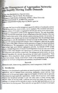
This document is an author's draft version submitted for publication to IEEE Sensors Journal. ... J. Raman, E. Cretu, P. Rombouts and L. Weyten, 'A Closed-Loop Digitally ..... resonant frequency, indicating a different sign for the parasitic.
1
A Closed-loop Digitally Controlled MEMS Gyroscope With Unconstrained Sigma-Delta Force-Feedback J. Raman, E. Cretu, P. Rombouts and L. Weyten
This document is an author’s draft version submitted for publication to IEEE Sensors Journal. The actual version was published as: J. Raman, E. Cretu, P. Rombouts and L. Weyten, ‘A Closed-Loop Digitally Controlled MEMS Gyroscope With Unconstrained Sigma-Delta Force-Feedback,” IEEE Sensors Journal, Vol. 9, No. 3, pp. 297-305, March 2009
1
A Closed-loop Digitally Controlled MEMS Gyroscope With Unconstrained Sigma-Delta Force-Feedback J. Raman, E. Cretu, P. Rombouts and L. Weyten
ABSTRACT In this paper we describe the system architecture and prototype measurements√of a MEMS gyroscope system with a resolution of 0.025 ◦/s/ Hz. The architecture makes extensive use of control loops, which are mostly in the digital domain. For the primary mode both the amplitude and the resonance frequency are tracked and controlled. The secondary mode readout is based on unconstrained Σ∆ force-feedback, which does not require a compensation filter in the loop and thus allows more beneficial quantization noise shaping than prior designs of the same order. Due to the force-feedback, the gyroscope has ample dynamic range to correct the quadrature error in the digital domain. The largely digital set-up also gives a lot of flexibility in characterization and testing, where system identification techniques have been used to characterize the sensors. This way, a parasitic direct electrical coupling between actuation and readout of the mass-spring systems was estimated and corrected in the digital domain. Special care is also given to the capacitive readout circuit, which operates in continuous time. 1. INTRODUCTION The development of high-performance micromachined gyroscopes is hindered by technology-related imperfections of the mechanical structure, which manifest themselves for instance in the existence of error components that largely exceed the signal to be measured (quadrature error). This imposes difficult requirements with respect to the dynamic range of readout and interface circuits. Also, the fact that mechanical parameters are unknown (due to fabrication variations, fluctuations with temperature and aging) poses serious challenges. These problems promote the use of closed-loop solutions. Moreover, it is beneficial to operate these control loops as much as possible in the digital domain. This allows the use of sophisticated signal processing techniques, and gives a lot of flexibility because improved techniques can be implemented, merely by changing the software. Following this philosophy, in the gyroscope described here, control loops are extensively used and migrated Manuscript received ——. J. Raman, P. Rombouts and L. Weyten are with Ghent University, Electronics and Information Systems (ELIS), St.-Pietersnieuwstraat 41, 9000 Ghent, Belgium. When this work was done, E. Cretu was with Melexis nv., Tessenderlo Belgium. He is now with the Dept. of Electrical and Computer Engineering, University of British Columbia, Vancouver, Canada. This work is supported by the Flemish Institute for Scientic and Technological Research (IWT) and developed in cooperation with Melexis NV, Transportstraat 1, 3980 Tessenderlo, Belgium.
as much as possible to the digital domain. With regard to the primary mode oscillation, a control loop is set up to track the resonant frequency of the mechanical structure while another loop stabilizes the amplitude. This way, temperature effects such as drift of the resonant frequency and the quality factor of the primary mode are neutralized. For the secondary (sense) mode the readout is based on Σ∆ force feedback [1–8]. This nearly inherently “digital” solution is fully compatible with our philosophy. An advantage of applying force-feedback to the secondary mode is that the dynamic range of the readout setup can be significantly improved. Indeed, by increasing the maximum attainable feedback force, larger input forces can be measured without saturating the readout and interface circuits (because these circuits only process the error signal). This increased dynamic range is important for dealing with the large parasitic forces causing the quadrature error. As will become clear, this digital set-up also gives a large flexibility in characterization and testing, where system identification techniques have been used to characterize the sensors. This way a parasitic direct electrical coupling between actuation and readout of the massspring systems was identified [9, 10]. Simply by modifying the demodulation algorithm this could be corrected for in the digital domain. Special care is also given to the capacitive readout circuit, which operates in continuous time. The rest of the paper is organized as follows. Section 2 describes the system architecture with its various control loops. Section 3 details the continuous time readout circuits. Experimental results are described in Section 4. Finally conclusions are presented in Section 5.
2. G YROSCOPE ARCHITECTURE A. System overview A system-level overview of the gyroscope as well as its physical partitioning is shown in Fig. 1. Three parts can be distinguished: first a micromechanical structure, which is implemented as a separate mechanical die (in dark grey on the figure). Second, there are analog interface electronics which are implemented in a separate ASIC (in medium grey on the figure), and finally digital functions (light grey). For ease of implementation and reconfiguration, an FPGA was used for the digital functions. The analog ASIC and the mechanical chip are wire-bonded and packaged in a single package.
2
This Coriolis force will act upon the mass spring system formed by the secondary mass and the secondary springs. By detecting this y-axis Coriolis force the angular velocity Ωz can be measured. In our approach, this is done by the use of forcefeedback on the secondary mode. For this purpose, the MEMS structure includes parallel-plate (variable gap) capacitors for both readout and actuation of the sense mode.
X-axis (primary) actuation
phase-sensitive
Coriolis force
demodulation quadrature error
x(t)
Fdrive
Tx(s) X
frequency loopfilter
DCO
primary-mode dynamics
cos sin
2dx/dt
X
amplitude controller
Wz
X
coupling through Coriolis force
sense mode x-axis SD position sense
y-axis SD position sense
force-feedback path
Y-axis (secondary) actuation
driven mode
driving force
cos sin
kyx
-2m
Fig. 1. System-level overview: mechanical sensor (dark grey), interface electronics (medium grey) and digital functions (light grey).
Fcor
parasitic mechancial cross-axis coupling cause of quadrature error
digital-domain SD modulator
y(t)
+ +
S
Ty(s) secondary-mode dynamics
Fig. 3. System level representation of the coupling between the primary mode and the secondary mode. Two coupling paths are apparent: (wanted) coupling through the Coriolis force, and parasitic mechanical coupling causing quadrature error.
W
Fig. 2. Simplified sketch of the dual-frame vibratory MEMS gyroscope. Anchored parts are in black, movable parts are in grey.
B. Review of Dual-frame vibratory gyroscopes The presented system-level approach of Fig. 1 can be applied in combination with many MEMS vibratory gyroscope structures. In our prototype, a dual-frame MEMS structure similar to [11–13] was used. The principle is reviewed in Fig. 2. First, an outer frame is suspended by primary mode springs in such a way that it can only move along the x-direction. Electrostatic comb drives are used to induce a vibratory motion: x(t) = X0 cos(ω0 t)
dx Ωz = 2mX0 ω0 Ωz sin(ω0 t) dt
C. Closed-loop control of the primary mode
(1)
Here, X0 is the amplitude of the primary motion, and ω0 denotes the pulsation, which is close to the resonance pulsation ωres of this mass-spring system. In order to be able to measure the amplitude X0 , a separate set of comb capacitors is used for readout. The primary mode movement is then translated to an inner mass by separate secondary mode springs. These are very stiff along the driven direction (x), but bend easily along the sense direction (y). Under influence of a z-axis rotation with an angular velocity Ωz , the secondary mass will experience a y-axis Coriolis force Fcor Fcor = −2m
Fig. 3 shows a system-level representation of the dynamics of the primary mode and its coupling to the secondary mode through the Coriolis force. Unfortunately in real-life gyroscopes, there is also a second coupling mechanism which is modelled as in e.g. [14] by the cross-axis spring coefficient kyx . This mechanism is also indicated in the figure and gives rise to an error. However, since this error is in quadrature with the Coriolis component, it can easily be separated from the Coriolis component by I/Q demodulation. Still this quadrature component is problematic, because it can be orders of magnitude larger than the Coriolis component. In an open-loop approach this would translate into unrealistic demands on the dynamic range of the readout circuit. In our gyroscope this problem is solved by the use of force-feedback which boosts the dynamic range and allows to correct for this quadrature error in the digital domain.
(2)
Fig. 4.
Diagram of the control loops for the primary mode.
A system-level diagram for the control of the primary mode is shown in Fig. 4. Here the mechanical structure is actuated by an electrostatic force Fact,x through the comb-drive actuators (Fig. 2). The primary mode responds to this force, resulting
3
in an x-displacement x(t). The force-to-displacement transfer function Tx (s) is described by the well-known mass-damperspring relationship: Tx (s) = ³
s ωres
+
s Qωres
a Fcor
+
S
_
Fact,y
Tm0 ´2
1
,
(3)
+1
where Tm0 corresponds with the mechanical DC-response. The x-displacement is measured by capacitive readout and converted to the digital domain by a conventional switchedcapacitor Σ∆ ADC. For optimal operation of the gyroscope, the primary mode should be operated at the resonance frequency ωres of the primary mass-spring system. To ensure this, the digitally controlled frequency is adjusted by the tracking loop until the displacement readout has 90 ◦ phase shift relative to the driving force. On the figure also a digital error compensation path is shown (in dashed lines), which is neglected for the moment and will be discussed in section 4A. A key component in this tracking loop is the digitally controlled quadrature oscillator (DCO), which has two exactly 90 ◦ phase shifted (digital) sinusoidal output signals, with a precisely matched amplitude. Here, the frequency resolution is an important specification, because it directly translates to phase noise of the frequency control loop (which is similar to a digital PLL). This is even more severe because of the high Q-factor of the primary mode (Q ≈ 100). Since phase errors are critical for correct demodulation (see underneath), in practice sub milli-Hz accuracy is needed. This is several orders of magnitude more accurate than what could be obtained by straightforward techniques such as simply dividing a high frequency master clock. The implemented DCO solution is therefore based on complex multiplication techniques, similar to [15]. For accurate gyroscope operation, also the amplitude should be well controlled. This is implemented here by an additional control loop. Note that, once the frequency control loop has settled, the amplitude of the primary mode can easily be obtained by projection on the sine-signal. The driving force is obtained from the cosine signal, rescaled to the amplitude dictated by the amplitude controller. This (multi-bit) digital signal is converted into a one-bit signal with a digital Σ∆modulator and further used for actuation. Depending on the binary value, an electrostatic force Fel is applied in either the positive or the negative x-direction: Fact,x = ±Fel . This is accomplished by applying a fixed voltage to the comblike actuator, which results in force pulses with constant magnitude, independent of the position of the proof mass in the x-direction. As a result, the actuation approach realizes an inherent digital-to-force conversion with good linearity. The mechanical structure reacts to this continuous sequence of force pulses (arriving at a high rate) in a frequency-selective way. Because of the resonant nature of the mechanical transfer of the primary mode, signals close to the resonant frequency are amplified (resulting in movement), while out-of-band frequencies are filtered out (and hence induce little motion). To make full use of this frequency-selective mechanism, the noise shaping of the digital Σ∆-modulator is optimized to push quantization noise as much as possible away from the
Fmax
y A 0
Ty(s)
readout secondary-mode gain dynamics mechanical feedback
1/4
+ _ S
_
1/2 +
-1
z
electrical 1/4 feedback
+ + _ S +
Dout
-1
z
one-bit quantizer
electrical 1/4 feedback
electrostatic zero-order hold pulse shaper actuation
Fig. 5.
Implemented unconstrained Σ∆ force-feedback architecture.
frequency range of interest (basically only a small band around the resonant frequency). D. Unconstrained Σ∆ Force-feedback for readout of the secondary mode As outlined above we use single-bit Σ∆ force-feedback for the readout of the secondary mode. However, it is well known that this approach gives rise to additional quantization noise. In order not to impose a cost in terms of resolution, quantization noise should be below the electronic noise of the readout front-end in the frequency-range-of-interest. Therefore, the transfer from quantization noise to the output of the Σ∆ forcefeedback loop — commonly called the noise transfer function (NTF) — should be carefully designed. In [8], a (theoretically) nearly optimal unconstrained architecture for such Σ∆ forcefeedback loops was presented, which is also employed here. A diagram of the used structure is shown in Fig. 5. Next to the mechanical transfer, an electrical resonator is added to the loop to provide a notch in the NTF at the operating frequency of the gyroscope. Similar to [3], the electrical resonator is built by applying local feedback (through the coefficient α) to a delaying and a non-delaying integrator. In our prototype the quantization noise is below the electronic noise in a bandwidth of 250 Hz around the gyroscope center frequency. E. Demodulation To determine the rotation rate Ωz , the digital output of the secondary mode is downconverted by multiplying with respectively the sine and cosine signal from the DCO. After lowpass filtering we obtain a Coriolis component DCor and a quadrature component DQ . From Eq. 2, it is clear that: −mX0 ω0 FCor = Ωz 2Fel Fel Clearly, the Coriolis component output DCor is proportional to the rotation rate Ωz . Furthermore the scale factor involved is well known. Indeed, the amplitude X0 of the primary mode is well controlled, and the oscillation frequency ω0 is exactly known since it is the DCO frequency. Also the electrostatic actuation force Fel is very stable with respect to temperature. Based on these arguments the scale factor drift over temperature is expected to be nearly zero. However, here we have assumed that all the control loops have perfect nullator operation. In practice this will only approximately be achieved, and thus we will have a very small but non zero temperature drift. DCor ≈
4
In practical gyroscopes, the quadrature error DQ is often very large. This puts severe constraints on the phase accuracy since even small phase errors will cause this quadrature error to leak to the Coriolis component. This is the main reason why a very high frequency resolution of the DCO is needed.
Anoise ≈ 1 +
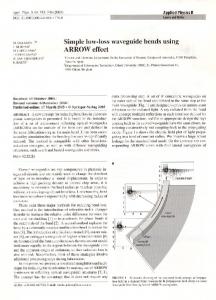
3. CT READOUT CIRCUIT Most analog circuit blocks are implemented with wellestablished switched-capacitor techniques and were partly reused from previous designs [16, 17]. However the capacitive readout circuit requires special care, because it is likely to limit the noise-performance. Inspired by the evolution in fully electrical Σ∆ modulators for A/D-conversion [18] where continuous-time circuitry has proven its capability of low-noise operation, a continuous-time (CT) readout seems promising for a low-noise operation of a gyroscope as well.
Fig. 6.
Here Cin corresponds to the input capacitance of the operational amplifier. In an optimized read-out circuit, the opamp’s input transistors are sized such that Cin is proportional to the parasitic capacitor Cp [20]: Cp (1 + α) . Cs
Here α is a design related proportionality constant which is sized α ≈ 1/3 in our circuit. As a result, for an optimized MEMS design, the parasitic capacitance Cp should be smaller than the sense capacitance Cs . In our design the capacitance of the secondary mode sense capacitor equals Cs = 1 pF. Unfortunately, the magnitude of the parasitic capacitance Cp , depends on technological constraints, which usually are not controlled by the MEMS designer. In our structure, Cp is larger than Cs , which leaves room for technological improvement.
Basic Continuous-time readout circuit based on a charge amplifier.
The basic principle of a continuous-time readout circuit is shown in Fig. 6. It consists of a fully differential operational amplifier with fixed feedback capacitors (CF B ). One side of both sense capacitors (Cs+ and Cs−) of the gyroscope structure are directly connected to the input terminals of the operational amplifier (nodes A and B). The common side of both sense capacitors (which is connected to the proof mass) is set at a fixed potential Vref . If we assume for the moment that the voltage at nodes A and B is controlled and equals VCM,in , then the differential output voltage Vout will equal: Cs+ − Cs− (Vref − VCM,in ), (4) CF B which indeed is proportional to the capacitance deviation. It is also proportional to the effective polarisation voltage (Vref − VCM,in ). In our case Vref = 0 Volt and VCM,in = 3 Volt. Since the capacitance variation is very small, it is clear that the feedback capacitor CF B should be small (≈ 200 fF) to have a good readout gain. The parasitic capacitors Cp are due to the fact that the sense capacitors of the mechanical die are wire-bonded to the electrical ASIC and hence these capacitors mainly consist of the parasitics of the bond-pads [19]. Unfortunately this capacitors are considerable in our gyroscope (≈ 6 pF), and have a significant impact on the noise of the readout circuit. Indeed, the input referred noise from the operational amplifier noise is amplified by a gain factor Anoise , which approximately equals: Vout ≈
Anoise = 1 +
Cp + Cin Cp + Cin + CF B ≈1+ Cs Cs
(5)
Fig. 7. Continuous-time readout circuit with large feedback resistors RF B to set the voltage at nodes A and B.
An important problem with the circuit of Fig. 6 is the fact that the input nodes of the opamp (nodes A and B) are floating, and hence their DC-component VCM,in is not controlled. A potential solution for this problem is to add large feedback resistors RF B as shown in Fig. 7 [21]. Here, the DC-voltage VCM,in is supplied through the resistors and will be equal to the output common mode voltage of the operational amplifier which is accurately controlled. Unfortunately, the charge amplifier now has a high-pass characteristic with a cut-off frequency fRC = 1/(2πRF B CF B ). The relevant readout signals will be centered around the mechanical resonance frequency fres of the gyroscope, which is of the order of 8 KHz. Obviously, for a good operation of the readout circuit these signals should be passed by the readout amplifier, which leads to a very large value (> 100MΩ) for the feedback resistor RF B , making a straightforward implementation of Fig. 7 impractical. The actually implemented circuit solution is shown in Fig. 8 and uses long-channel FET’s [21] to achieve a resulting equivalent feedback resistance RF B of the order of 100 MΩ. This is not large enough to pass the gyroscope signals, centered around fres , unaffected. The main effect of this is a phase shift. In an open-loop readout (as in [21]), this would be unacceptable. Therefore, in [21], the equivalent feedback resistance is further boosted by keeping the triode-FET switched off most of
5
the switching event, because of its reduced bandwidth.
Fig. 8. Continuous-time readout circuit with a triode operated transistor and 1-order filter. Fig. 10. Transfer Vout /x of the readout circuit. Note that the gyroscope signal located at fres = 0.02 ∗ f sample is passed.
the time and only switching it on with a low duty cycle. This technique is not readily applicable in a Σ∆ force feedback loop, because it would cause aliasing of quantization noise due to the inherent subsampling involved. Fortunately, in our closed-loop architecture, a phase shift of the readout circuit is not a major problem, because it is inside the force feedback loop. The lowpass filter is inserted, because in our architecture of the Σ∆ force feedback loop, the output of the readout amplifier is not extremely small. To avoid that the long-channel FET’s leave the triode region, the signal at the FET’s drain is attenuated by the lowpass filter, ensuring correct operation. The implemented lowpass-filter is a standard passive firstorder switched-cap filter.
Fig. 9. Fully differential operational amplifier with a telescopic cascode and source follower output buffers.
The schematic of the operational amplifier is shown in Fig. 9. It consists of a first telescopic cascode stage, loaded with the compensation capacitors CC . These capacitors set the bandwidth of the operational amplifier. Here, the bandwidth is set as low as possible, to filter out most high-frequency noise of the readout amplifier which would otherwise alias back to the signal band. This leads to a bandwidth approximately equal to the sample frequency (∼ 400 kHz). The source followers at the output are needed, because the readout amplifier is loaded by the switched capacitors of the electrical resonator in the force feedback loop (Fig. 5). Without these buffers the output of the readout amplifier cannot recover in time from
The transfer function of the readout amplifier is shown in Fig. 10. As explained above, both low-frequency and highfrequency signals are rejected while the gyroscope signal at 8 KHz is passed. Due to the dynamics of the lowpass filter, there is some out-of-band, low-frequency peaking but this does not affect the force-feedback operation. The discussion above was focused on the readout of the secondary mode, which is the most critical, but a similar circuit is used in the primary mode readout as well. 4. E XPERIMENTAL RESULTS The complete gyroscope system according to Fig. 1 was designed and implemented. For this purpose a prototype ASIC containing the analog circuits was designed and fabricated in a 0.6 µm CMOS process with a high-voltage (18 V) option, needed for the actuation. This ASIC was wire-bonded to the mechanical chip containing a differential version of the dual-frame gyroscope structure sketched in Fig. 2. The same mechanical die as in [6] was used. A microscope photograph of the package containing the two dies is shown in Fig. 11. This chip was assembled on a standard printed circuit board and connected to an FPGA containing all the digital blocks. For the measurements reported here, all circuits are clocked at a fixed master clock frequency (400 kHz).
Fig. 11. Microscope photograph of the wire-bonded dies of the analog ASIC and the mechanical chip.
6
0
Mechanical response -10
dB
-20
-30
-40
Fig. 13.
Notch
Mechanism for frequency independent coupling.
-50 0.014
0.016
0.018 0.02 0.022 Normalized Frequency f/fSample
0.024
layout will cause a systematic difference between Ccouple,A and Ccouple,B , leading to the observed coupling effect. To take this effect into account an additional coupling term Te0 has to be added to the overall sensor transfer function Tsens :
0
-10
Tsens = ³
dB
-20
-30
-40
-50 0.014
Mechanical response Total response 0.016
0.018 0.02 Normalized frequency f/f
0.022
0.024
Sample
Fig. 12. Response to pseudo-noise actuation of the primary mode: measured (top) and calculated from the identified system (bottom). Also shown on the bottom figure is the expected mechanical response (without the parasitic electrical coupling).
A. System identification For the primary mode we expect a mechanical response Tx according to Eq. (3). However, the actual sensor transfer characteristic may deviate from this, e.g. due to direct electrical coupling [9, 10]. One of the assets of our largely digital setup is that it is easy to perform a system-level identification procedure. To do this for the primary mode, the primary mode control loops (which are entirely digital) are broken, and a single-bit white pseudo-noise actuation signal is applied. The corresponding response is obtained from the (digital) output. Fig. 12 (top) displays the result. One can clearly distinguish a peak, which corresponds to the mechanical resonance. However, also a notch can be seen. This notch is attributed to a parasitic electrical coupling directly from actuation to readout [9, 10]. In the literature both frequency dependent [10] and independent coupling mechanisms have been reported. In our gyroscope, the system identification revealed that the coupling could be considered frequency independent. The basic mechanism for frequency independent coupling is sketched in figure 13 and is caused by parasitic (layout) capacitors Ccouple,A and Ccouple,B connecting the actuation voltage to the input nodes of the capacitive readout amplifier (described in section 3). Mismatch in the
s ωres
´2
Tm0 + Te0 . ³ ´ + Qωsres + 1
(6)
From a curve fit on the measured curve (Fig. 12, top), the coupling term was estimated and it was confirmed that Te0 is a constant, in agreement with a frequency-independent coupling mechanism. Based on the estimated value of Te0 the theoretically matched curve was calculated and is shown in Fig. 12 (bottom, bold curve). It is clear that the measured and the theoretical curve match well. Without the parasitic electrical coupling, the dotted curve would be valid. It is clear that the magnitude of the resonance peak is not substantially affected by the parasitic electrical coupling. However, the induced phase shift is problematic because it results in a phase error in the I/Q demodulation of the Coriolis/Quadrature component which causes the large quadrature error to leak to the demodulated Coriolis component. Therefore, in our implementation the parasitic electrical coupling is compensated in the digital domain, by adding the error compensation path to the primary mode frequency tracking loop (see Fig. 4).
a
Fig. 14. Configuration for system identification of the secondary mode, by reconfiguring the force feedback loop of Fig. 5.
Also for the secondary mode a system identification can be performed. To do this, the feedback loop of Fig. 5 is rearranged by disabling the mechanical feedback path and instead driving the actuator with a a single-bit white pseudo-noise signal. The resulting system is shown in Fig. 14. Now the configuration consists of a cascade of the sensor with a plain electrical Σ∆ ADC. Note that this can not easily be done with alternative Σ∆
7 Spectrum of the primary mode digital readout 40
force-feedback configurations which have only mechanical feedback [8].
30 20
25
10 0
20
-10
dB
15
-20
10
dB
-30
5
-40
0
-50 -60
-5
-70 -4 10
-10
-3
10
-2
10 Normalized Frequency f/fSample
-1
10
-15
Fig. 16. Measured spectrum of the digital output bitstreams for the primary mode (100× averaged 64K FFT).
-20 -25
0.01
0.015
0.02
0.025
0.03
0.035
0.04
0.045
Normalized Frequency f/fSample
In Fig. 16 the result for the primary mode is shown. Before starting the measurements, the frequency-tracking loop has been activated long enough to allow the system to lock onto the resonant frequency of the primary mode. Also the amplitude of the driving signal is set to stabilize the primary mode amplitude to a fixed value. One clearly sees the strong signal at the normalized frequency 0.02, which represents the primary mode excitation. Next to this, the shaping of the quantization noise (with a notch at the resonant frequency) is prominently present. This quantization noise comes in part from the readout Σ∆ ADC and in part from the driving Σ∆ DAC (see Fig. 4).
25 20 15 10
dB
5 0 -5 -10 -15
Mechanical response Total response
-20 -25
0.01
0.015
0.02
0.025
0.03
0.035
0.04
0.045
30
Normalized Frequency f/fSample
20 10
Fig. 15. Response to pseudo-noise actuation of the secondary mode: measured (top) and calculated from the identified system (bottom). Also shown on the bottom figure is the expected mechanical response (without the parasitic electrical coupling).
0 -10
dB
-20
Fig. 15 displays the results for the secondary mode. Again, a peak in the response corresponding to the mechanical resonance can be noted. Also here, a notch can be seen, which again is caused by a parasitic electrical coupling (Eq. 6). However, this time the notch is located to the right of the resonant frequency, indicating a different sign for the parasitic electrical coupling. This difference in sign with the primary mode is due to differences in the layout parasitics which are different for both modes. Fortunately the direct parasitic coupling path in the secondary mode does not significantly alter the performance of the gyroscope. To understand this, we first observe that this transfer function is in the forward path of the force feedback loop. Hence it will not alter the nullator operation of the feedback loop, provided the loop remains stable. And we have verified that the electrical coupling does not alter the stability of the feedback loop.
-30 -40 -50 -60 -70 -80 -90 -4 10
10
-3
10
-2
-1
10
Normalized Frequency f/fSample
Fig. 17. Measured Spectrum of the secondary mode digital output bitstream (100× averaged 64K FFT).
In Fig. 17, a typical spectrum of the readout of the secondary mode force-feedback loop is shown. The tone at 0.02fsample corresponds to the measured force at the secondary mode, which consists of a Coriolis component and a quadrature component. C. Gyroscope characteristics
B. Noise shaping characteristics To evaluate the noise shaping in both Σ∆ loops the output bitstreams of both the primary and secondary mode are converted into the frequency domain.
Fig. 18 shows the measured Coriolis component vs. the applied rotation Ωz . For this measurement the gyroscope system was mounted on a rotation table, and the rotation was varied over the interval [-150; +150] ◦/s. Obviously the characteristic is
measured rotation rate (LSB)
8
-500
Linearity Scale factor drift
primary mode: Qx ≈ 100 sense mode: Qy ≈ 15 analog blocks: 5 Volt comb drive voltage: 18 Volt 250 µA@5 Volt 100 µA@18 Volt > 1100 ◦/s measured > 4000 ◦/s theoretical < 0.25 ◦/s in range [−150 ◦/s, +150 ◦/s] < 0.01%/ ◦ C
-1000
Zero rate drift Bandwidth
< 0.023 ◦ C > 100Hz
-1500
Noise floor Quadrature Error
0.025 √ Hz 675 ◦/s
1500
Mechanical Q-factors
1000
Supply Voltages
500
Current consumption Full scale range
0 -150
-100
-50
0
50
100
150
applied rotation rate (°/s)
◦
/s
◦
/s
TABLE I Fig. 18. Global gyroscope characteristic, showing the relation between the rotation rate readout versus the applied rotation rate. Dots indicate different measurements.
visually linear. The result of a best line fit on the measurements of Fig. 18, indicates that the non-linearity is less than |0.25| ◦/s. However this is beyond the accuracy of the rotationrate control of our rotation table, so we assume the actual linearity is better. There is also a small offset of −2.1 ◦/s, which of course can be removed by a zero-rate calibration. The full scale range could not be measured reliably, with our equipment. By disabling the rotation-control of the rotation table, and having the table turn at its maximum speed, we have verified that the full scale range is > 1100 ◦/s. Actually, simulations and calculations indicate that the full scale range is even a lot higher and well above 4000 ◦/s, but with our measurement setup we could not confirm this experimentally. For these measurements the quadrature error DQ was monitored as well, and it was found that its magnitude corresponds to DQ = 675 ◦/s, nearly independent of the applied rotation rate. For an open-loop readout of the secondary mode, this would obviously give overloading problems, but due to force feedback, the signal range is more than sufficient to correct this in the digital domain. The gyroscope noise floor ◦ . This was measured as well and turned out to be 0.025 √/s Hz noise level compares favorably with other recently published gyroscopes [3, 21–23]. The presented design techniques are also fully compatible with mode-matching techniques such as in [23].A modified design that combines these techniques could achieve an even lower noise level. We do not have the equipment to perform an accurate temperature characterization. All the measurements reported above, were done at room temperature, but we performed some basic temperature measurements where the gyroscope was exposed to a hot air stream (controlled at 100 ◦ C). From this measurement we could verify that the scale factor drift is ◦ . A < 0.01%/ ◦ C and that the zero rate drift is < 0.023 ◦/s C summary of the above measurement results is shown in table I.
S UMMARY OF GYROSCOPE CHARACTERISTICS
5. C ONCLUSIONS We have presented the circuits and system-level concepts for a MEMS vibratory gyroscope as well as experimental results. Key features are a continuous time capacitive readout amplifier and the extensive migration of control tasks to the digital domain. The primary oscillation is controlled by both a resonance frequency tracking as well as an amplitude loop. For the secondary mode an unconstrained Σ∆ force feedback loop is used. The setup gives the possibility to perform extensive system identification during experimental testing. Here a direct coupling from the electrical actuation to the electrical readout was found. The resulting overall gyroscope system has a ◦ . Thanks to the use of force-feedback noise floor of 0.025 √/s Hz the dynamic range (theoretically > 4000 ◦/s) greatly exceeds the requirements for a fully digital correction of the large quadrature error. ACKNOWLEDGMENT This work is supported by the Flemish Institute for Scientific and Technological Research (IWT). The authors wish to thank XFab for fabrication of the silicon, and the Melexis Inertial Sensors Business Unit for giving permission to publish this material. R EFERENCES [1] M. Lemkin and B. E. Boser, “A three-axis micromachined accelerometer with a CMOS position-sense interface and digital offset-trim electronics,” IEEE J. Solid-State Circuits, vol. 34, no. 4, pp. 456–468, Apr. 1999. [2] Y. Dong, M. Kraft, C. Gollasch, and W. Redman-White, “A highperformance accelerometer with a fifth-order Σ∆ modulator,” J. Micromechanics and Microengineering, vol. 15, no. 7, pp. 22–29, Jul. 2005. [3] V. P. Petkov and B. Boser, “A fourth-order Σ∆ interface for micromachined inertial sensors,” IEEE J. Solid-State Circuits, vol. 40, no. 8, pp. 1602–1609, Aug. 2005. [4] V. P. Petkov and B. E. Boser, “High-Order Electromechanical Σ∆ Modulation in Micromachined Inertial Sensors,” IEEE Trans. Circuits Syst.-I, vol. 53, No. 5, pp. 1016-1022, May 2006. [5] H. K¨ulah, J. Chae, N. Yazdi, and K. Najafi, “Noise analysis and characterization of a Sigma-Delta capacitive microaccelerometer,” IEEE J. Solid-State Circuits, vol. 41, no. 2, pp. 352–361, Feb. 2006. [6] J. Raman, E. Cretu, P. Rombouts and L. Weyten, “A Digitally Controlled MEMS Gyroscope With Unconstrained Sigma-Delta Force-Feedback Architecture,” Proc. 19th IEEE Int. Conf. on Micro Electro Mechanical Systems, Istanbul, pp. 710-713, Dec. 2006.
9
[7] Y. Dong, M. Kraft and W. Redman-White, “Micromachined vibratory gyroscopes controlled by a high-order bandpass sigma-delta modulator,” IEEE Sensors Journal, Vol. 7, No. 1-2, pp. 59-69, Jan-Feb 2007 [8] J. Raman, P. Rombouts and L. Weyten, ”An Unconstrained Architecture for Systematic Design of Higher-Order Σ∆ Force-Feedback Loops,” IEEE Trans Circuits Syst.-I, accepted for publication, avialable online at ieeexplore [9] S. Alper and T. Akin, “A single-crystal silicon symmetrical and decoupled MEMS gyroscope on an insulating substrate,” J. Microelectromechanical Systems, Vol 14, No. 4, pp. 707-717, Aug. 2005 [10] C. Acar and A. M. Shkel, “An approach for increasing drive-mode bandwidth of MEMS vibratory gyroscopes,” J. Microelectromechanical Systems, Vol 14, No. 3, pp. 520-528, Jun. 2005 [11] W. Geiger, W. Butt, A. Gaisser, J. Frech, M. Braxmaier, T. Link, A. Kohne, P. Nommensen, H. Sandmaier, W. Lang and H.Sandmaier, “Decoupled microgyros and the design principle DAVED,” Sensors and Actuators A-Physical Vol. 95, No. 2-3, pp. 239-249, Jan. 2002 [12] Moorthi Palaniapan, Roger T. Howe and John Yasaitis, “Integrated Surface-Micromachined Z-axis Frame Microgyroscope,” in IEDM Digest. International Electron Devices Meeting, pp. 203-206, dec, 2002. [13] Moorthi Palaniapan, Roger T. Howe and John Yasaitis, “Performance Comparison of Integrated Z-axis Frame Gyroscopes,” in MEMS-03 - The Sixteenth Annual International Conference on Micro Electro Mechanical Systems, pp. 482-485, jan, 2003. [14] M. Saukoski, L. Aaltonen, K. Halonen, “Zero-rate output and quadrature compensation in vibratory MEMS gyroscopes,” IEEE Sensors Journal, vol. 7, No. 11-12, pp. 1639-1652, Nov-Dec 2007 [15] K. Palomaki, J. Niittylahti and M. Renfors, “Numerical sine and cosine synthesis using a complex multiplier,” Proc. of IEEE Int. Symp. Circuits and Syst. (ISCAS), Vol. 4, pp. 356 - 359, Jul 1999 [16] P. Rombouts, J. De Maeyer and L. Weyten, “ A 250-kHz, 94-dB doublesampling Σ∆ modulation A/D converter with a modified noise transfer function,” IEEE J. Solid-State Circuits, vol. 38, No. 10, pp. 1657-1662, Oct. 2003. [17] J. De Maeyer, P. Rombouts and L. Weyten, “A Double Sampling Extended Counting ADC,” IEEE J. Solid-State Circuits, vol. 39, No. 3, pp. 411-418, Mar. 2004. [18] L. Breems, E. van der Zwan and J. Huijsing, “A 1.8-mW CMOS Σ∆ Modulator with integrated Mixer for A/D Conversion of IF signals,” IEEE J. Solid-State Circuits, vol. 35, No. 4, pp. 468-475, Apr. 2000. [19] T. Kajita, U.-K. Moon, and G. Temes, “A two-chip interface for a MEMS accelerometer,” IEEE Trans. Instrumentation and Measurement, vol. 51, no. 4, pp. 853 – 858, Aug. 2002. [20] J. F. Wu, G. K. Fedder, L. R. Carley, √ “A low-noise low-offset capacitive sensing amplifier for a 50-µg/ Hz monolithic CMOS MEMS accelerometer,” IEEE J. Solid-State Circuits, vol. 39, No. 5, pp. 722730, May 2004 [21] J. Geen, S. Sherman, J. Chang and S. Lewis, ”Single-chip surface micromachined integrated gyroscope with 50 degrees/h allan deviation,” IEEE J. Solid-State Circuits, vol. 37, No. 12, pp. 1860–1866, Dec. 2002; [22] M. Saukoski, L. Aaltonen, K. Halonen and T. Salo, “Integrated Readout and Control Electronics for a Microelectromechanical Angular Velocity Sensor,” Proc. EssCirc. 2006, pp. 243-246, Sept. 2006. [23] C. D. Ezekwe and B. E. Boser, “A mode-matching √ ∆Σ closed-loop vibratory-gyroscope readout interface with a 0.004/s/ Hz Noise floor over a 50Hz band,” in ISSCC Dig. Tech Papers, Feb. 2008, pp. 580-581.
Johan Raman Johan Raman was born in Ghent, Belgium, in 1970. He received the Ir. and Ph.D. degrees in electronics from Ghent University, Ghent, Belgium, in 1993 and 2000, respectively. In 1994, he joined the Department of Electronics and Information Systems, Ghent University. His technical interests are signal processing, circuits and systems theory, analog circuits, and MEMS sensor design. His research is currently focused on MEMS inertial sensors.
Edmond Cretu Dr. Cretu received the Ph.D. degree in Electrical Engineering from Delft Technical University, The Netherlands, in 2003. He previously held a researcher position in Romanian Academy (1990-1994), and later worked as Senior Designer and Project Manager for Melexis, Belgium (20002005). Since 2005, Dr. Cretu is Assistant Professor in the Dept. of Electrical and Computer Engineering, University of British Columbia.
Pieter Rombouts Pieter Rombouts was born in Leuven, Belgium in 1971. He obtained the Ir. degree in applied physics and the Dr. degree in electronics from Ghent University in 1994 and 2000 respectively. Since 1994 he has been with the Electronics and Information Systems Department of the Gent university where he is currently professor. In 2002 he was a visiting professor at the University Carlos III in Madrid (Spain). His technical interests are signal processing, circuits and systems theory and analog circuit design.
Ludo Weyten Ludo Weyten was born in Mortsel (Antwerpen, Belgium) in 1947. He received the Ir. degree and the Dr. degree from Ghent University (Belgium) both in Electrical Engineering, in 1970 and 1978 respectively. From 1970 to 1972 he joined the Electronics Laboratory of the same university as a research assistent. From 1972 to 1975 he was teaching at the National University of Za¨ıre (now Congo) at Lubumbashi in a government technical co-operation project. Since 1975 he is with the Engineering Faculty of Ghent University (Belgium) where he is currently professor. His teaching and research interests are in the field of electronics circuits and systems and e-learning.