The International Archives of the Photogrammetry, Remote Sensing and Spatial Information Sciences, Volume XLII-3, 2018 ISPRS TC III Mid-term Symposium “Developments, Technologies and Applications in Remote Sensing”, 7–10 May, Beijing, China
A CLOUD BOUNDARY DETECTION SCHEME COMBINED WITH ASLIC AND CNN USING ZY-3, GF-1/2 SATELLITE IMAGERY Zhengsheng Guo 1,2,*, Canhai Li 2, Zhimin Wang 1, Expo Kwok 1, Xu Wei 1 1
2
School of Geomatics, Liaoning Technical University, Fuxin 123000,China -
[email protected] Satellite Surveying and Mapping Application Center, National Administration of Surveying, Mapping and Geoinformation, Beijing 100048, China
KEY WORDS: CNN, ASLIC, GF-1/2, ZY-3, Imaging platforms ABSTRACT: Remote sensing optical image cloud detection is one of the most important problems in remote sensing data processing. Aiming at the information loss caused by cloud cover, a cloud detection method based on convolution neural network (CNN) is presented in this paper. Firstly, a deep CNN network is used to extract the multi-level feature generation model of cloud from the training samples. Secondly, the adaptive simple linear iterative clustering (ASLIC) method is used to divide the detected images into superpixels. Finally, the probability of each superpixel belonging to the cloud region is predicted by the trained network model, thereby generating a cloud probability map. The typical region of GF-1/2 and ZY-3 were selected to carry out the cloud detection test, and compared with the traditional SLIC method. The experiment results show that the average accuracy of cloud detection is increased by more than 5%, and it can detected thin-thick cloud and the whole cloud boundary well on different imaging platforms. 1. INTRODUCTION China started to launch domestic high-resolution optical remote sensing satellites ZY-3 and GF-1/2 in 2012. However, as more than 50% of the Earth's surfaces is covered by clouds, a large number of optical images contain clouds, reducing the utilization of images. Therefore, cloud detection and elimination become one of the hot topics in the field. Early cloud detection methods are mainly based on the albedo of the cloud in different spectrum segments, and select the appropriate threshold for cloud recognition. Di Girolamo and Davies proposed an improved cloud detection method based on NDVI for aerial images of the Airborne Visible Infrared Imaging Spectrometer (AVIRIS). This method can effectively identify the thick cloud, but the detection effect of the thin cloud is very poor. For example, during the cloud detection of QuickBird images, the lake was misjudged as a thin cloud. Janmes J. Simspon et al.used cloud shadow effect and combined with AVHRR five-channel data to achieve cloud detection of NOAA meteorological satellites. This method is greatly influenced by the sun zenith angle. In 2011, Italian scholar Riccardo Rossi and others used the singular value decomposition (SVD) technology to extract the features of the image and applied support vector machine (SVM) classifier to detect QuickBird satellite image cloud detection. This method achieves cloud detection for high-resolution remote sensing satellites. However, simple SVD only constructs feature vectors from the grayscale statistical distribution point of view that cannot describe the attributes of the cloud in an all-round way. In remote sensing images, the thickness and shape of the cloud layer are varied. Most of the existing cloud detection methods only extract the low-level features of the cloud, so it is difficult to adapt to the complex remote sensing images, especially the thin clouds under the low contrast background. Yu Q proposed a natural image classification algorithm based on a large deep convolution neural network, which has obtained high classification accuracy on the ImageNet dataset. CNN is one of the typical deep learning algorithms, and the parameters in the CNN model are obtained by network training through gradient
descent method. Trained CNN can fully excavate the features of the image, and finally complete the classification of remote sensing image. In this paper, a cloud detection method based on CNN is proposed for domestic optical images. Firstly, ASLIC method is used to clustering homogeneity pixels to be superpixels; Secondly, the multilevel features of the cloud are extracted by using the dual-branch CNN network to obtain the model. Finally, the superpixel input model generates a cloud probability map. The rest of the paper is organized as follows: Section II introduces the method of cloud detection; Section III is verified through the experiment; Section IV summarizes the full text. 2. OUR APPROACH In this section, we introduce the details of the deep learning cloud detection method. Figure 1 shows flowchart of the proposed method. It is the process of inputting superpixel into CNN model to obtain a cloud probability map. High ASLIC resolution image
Superpixel subregion
CNN Model
Could probability map
Refine
Cloud detection results
Figure 1. Flowchart of the proposed method 2.1 CNN structure CNN is one of the pioneering research results inspired by the knowledge of biological neurology and reference to its structural principles combined with artificial neural networks. It has the advantages of local area perception, space or time sampling and weight sharing, which greatly reduces the training parameters of global optimization. At present, it has become a hot topic in the field of deep learning such as image classification, object detection and face identification. CNN structure consists of input layer, convolutional layer, and fully connected layer. Figure 2 shows a simplified schematic diagram of the CNN structure.
* Corresponding author: Guo Zhengsheng E-mail addresses:
[email protected]
This contribution has been peer-reviewed. https://doi.org/10.5194/isprs-archives-XLII-3-455-2018 | © Authors 2018. CC BY 4.0 License.
455
The International Archives of the Photogrammetry, Remote Sensing and Spatial Information Sciences, Volume XLII-3, 2018 ISPRS TC III Mid-term Symposium “Developments, Technologies and Applications in Remote Sensing”, 7–10 May, Beijing, China
Figure 2 Single branch CNN structure In this paper, we design a dual-branch CNN structure to complete the classification task of multi-level cloud, and classify the image blocks that need to be classified into three categories: thin cloud, thick cloud and non-cloud. Figure 3 shows the overall architecture of CNN. In this work, we need to
in55data
In55conv1 in55relu1
In55conv2 in55relu2
in55pooling1
divide the images into three classes, so the number of classes on the last layer of CNN is 3. In Figure 3, conv# is defined as convolutional layer, relu# as a nonlinear rectified linear unit function, pooling# is defined as pooling layer, concat# as a merger layer, fc# as a fully connected layer.
in55pooling2
In55conv4 in55relu4
In55conv3 in55relu3
CNN Net
Loss
conv1 relu1
data
pooling1
conv2 relu2
pooling2
conv3 relu3
conv4 relu4
pooling5
in55fc6 in55relu6 in55drop6
in55pooling5
fc7 relu7 drop7
fc8
fc6 relu6 drop6
Concat
Figure 3 The architecture of our designed CNN 2.2 ASLIC algorithm
d s (x j y i ) 2 (y j y i ) 2
Achanta R proposed simple linear iterative clustering (SLIC) based on color and spatial distance in 2010. This method generates superpixels by modifying the traditional K-means clustering algorithm. It transforms the color image into CIELAB color space and XY coordinates to form a fivedimensional feature vector,and then performing pixel partial clustering optimization by constructing the distance metrics for the five-dimension feature vector. The SLIC implementation steps are as follows: 1) Initialize the seed. Assuming that the image has N pixels, the method pre-divides the image into K superpixels of the same size, and the size of each superpixel is N/K, and the distance between the center points of each superpixel is approximately represented as S N / K . 2) Update the seed. In order to avoid the seed points falling on the gradient boundary, the seed points are transferred to the smallest pixel gradient in the 3×3 neighborhood. The calculation formula of the gradient is:
G ( x, y ) || I (x 1, y) I (x 1, y) ||2 (1)
|| I (x, y 1) I (x, y 1) ||
2
3) Assign a label. Assign a class tag to all pixel points in the neighborhood of each seed point. 4) Distance metrics. Including color distance and space distance. For each searched pixel, calculate its distance from the seed point separately. The distance measurement between the ith pixel and the j-th cluster center is defined as:
d c (l j l i ) (a j a i ) (a j a i ) 2
2
2
(2)
(3)
2
d D dc 2 s m2 S
(4)
Where dc and ds are the color difference and spatial distance between pixels, the weight m representing the ratio of color similarity to spatial proximity. 5) Iterative optimization. Repeat the above steps until the convergence error is less than a certain threshold. 6) Increase connectivity. For multi-connected, discontiguous,oversized superpixels appearing in the segmentation result, the labels of the largest neighboring clusters are reassigned to the neighboring superpixels. As shown in Figure 4(b), SLIC algorithm has a high overall evaluation in terms of operation speed, object contour preservation and superpixel shape, but the generated superpixels are difficult to maintain compactness and homogeneity. As shown in Figure 4(c), ASLIC adaptively selects the compact- ness factor and the superpixel step length. The rule shape superpixel will be produced in both the texture and the non texture regions. ASLIC dynamically normalizes the proximities for each cluster using its maximum observed spatial and color distances (ms, mc) from the previous iteration. Thus, the distance measure becomes: 2
d d D c s mc ms
2
(5)
In this way, the compactness of the superpixel is more consistent and does not need to set up m.
This contribution has been peer-reviewed. https://doi.org/10.5194/isprs-archives-XLII-3-455-2018 | © Authors 2018. CC BY 4.0 License.
456
The International Archives of the Photogrammetry, Remote Sensing and Spatial Information Sciences, Volume XLII-3, 2018 ISPRS TC III Mid-term Symposium “Developments, Technologies and Applications in Remote Sensing”, 7–10 May, Beijing, China
(a) (b) (c) Figure 4. An instance of initial cluster center generation. (a) Original RGB image. (b)SLIC (C)ASLIC 3. EXPERIMENTAL RESULTS In order to verify the effectiveness of the proposed cloud detection scheme, we compare with Shi’s proposed SLIC cloud detection method. The algorithm is implemented in the hardware environment of Intel (R) Xeon (R) CPU W3565 @ 3.20GHz 3.19GHz Ubuntu14.04 system and it's achieved by the deep learning framework caffe.Considering the research area of cloud distribution, we choose the 5 scenes of ZY-3 and GF-1/2 datasets with cloud content exceeding 20% from June to October in the southern China on the ZY-3 Image Cloud Service Platform(http://sasclouds.com/query). Among them, the ZY-3 image is a multi-spectral data with spatial resolution of 5.8 meters, and the GF-1/2 image is about 1m of the spatial resolution after preprocessing. Among them, the criteria for the differentation of thin and thick clouds: through the visual observation of the cloud area, the bright white place is thick cloud, thin and fuzzy are thin clouds. Small pieces of 55 × 55
and 111× 111 are extracted by manually using each pixel at the center of the image as a training sample. Similarly, from the three types of image data, 10 non-training regions with a size of 500×500 to 800×800 images were used for testing. The construction of the network structure model is shown in Figure 3. It contains eight layers. The first four layers are the convolution layer, the middle is the concat layer, and the other three layers are fully connected. The convolution filter is set to 48, 64, 128 and 256, and the filter size is set to 5×5. The pooling interval is set to 2, the CNN activation function is nonlinear rectified linear unit function (ReLu). Finally, the CNN learning multi-level cloud feature is input to SVM classifier for cloud detection. Our method cloud detection results are shown in Figure 5(d). Shi’s cloud results are shown in Figure 5 (c).
(a)Original image (b) Ground truth (c) SLIC (d) the proposed method Figure 5. Visual comparisons of different methods on cloud detection.
This contribution has been peer-reviewed. https://doi.org/10.5194/isprs-archives-XLII-3-455-2018 | © Authors 2018. CC BY 4.0 License.
457
The International Archives of the Photogrammetry, Remote Sensing and Spatial Information Sciences, Volume XLII-3, 2018 ISPRS TC III Mid-term Symposium “Developments, Technologies and Applications in Remote Sensing”, 7–10 May, Beijing, China
In Figure 5, the first and second lines correspond to the images of the ZY-3 and the GF-1. Between the two images with high contrast background cloud. Although the two methods can obtain correct cloud area, our method can obtain more accurate boundaries. The third line in Figure5 is the GF-2 image. The ground is complex and has bright areas in the background. For these complicated situations, the results of SLIC cloud detection results 5(c) have been mistaken and missed, and some objects such as bare ground and white buildings are mistaken for cloud. In our method, there is no false inspection and leakage. Through visual evaluation, we can find that the cloud boundary is clear in the results of our cloud detection, and it can identify the boundaries between thin and thick clouds. In order to quantitatively evaluate the cloud detection method, the cloud region which is extracted by artificial visual interpretation is used as the true value. It's sketching criteria: the precision of the cloud boundary blur region is within 2 pixels, and the precision of the cloud boundary clear region is within 1 pixels. The algorithm is measured quantitatively with three indicators. They are the accuracy rate(RR), error rate(ER) and false alarm rate (FAR). The calculation formula of the three indicators is as follows:
RR Where
CC CN NC NC ; ER ; FAR GN TN GN
(6)
CC=correctly detected as a cloud GN=ground truth cloud pixels CN=cloud pixels detected as non-cloud pixels NC= non-cloud pixels detected by cloud pixels TN=the total number of pixels in the input image.
The above three indicators RR, ER and FAR are used to quantitatively evaluate the effectiveness of different methods. Because the comparison method cannot distinguish between thin and thick clouds, only the entire detected cloud area is evaluated in the results. Table 1 gives the average of the results of 30 test images. Considering the three indicators in Table 1, it can be seen that the precision of our detection and placement is higher than that of the traditional SLIC. The accuracy of the correct detection is 0.9483, which is 5.65% higher than that of the traditional SLIC algorithm. At the same time, both ER and FAR are lower than the traditional SLIC, which means that our solution can effectively improve cloud detection accuracy in domestic satellite image. Table 1. Statistics the results of RR、ER and FAR for different cloud detections RR ER FAR SLIC 0.8918 0.0649 0.0981 ASLIC 0.9483 0.0058 0.0104 4. CONCLUSION This paper focuses on the deep learning of current research hotspots and proposes a cloud detection method for domestic optical remote sensing images combined with ASLIC algorithm. This method can autonomously separate the cloud into compact and uniform superpixels, and avoid the weak segmentation phenomenon caused by artificial selection parameters. By in putting superpixel to the CNN model for prediction, we can get the probability map belonging to the cloud area. In the process of testing, the method is robust to the detection of thin clouds in
complex background features such as buildings, bare land, snow and so on. Experimental results show that the method is feasible for cloud detection with less misjudgement, suitable for the cloud and cloudless images, and the average overall detection accuracy rate of more than 94%, and it is also suitable for cloud detection of different imaging platform images. In addition, limited by the number of thin clouds training samples and the boundary of thin-thick clouds, We are not very good at detecting thin cloud in the edge of thick cloud. After that, we will focus on how to improve the accuracy of such thin cloud based on existing magnitude training samples. 5. REFERENCES Paltridge G W, Platt C M R., 1976. Radiative processes in meteorology and climatology[M]// Radiative processes in meteorology and climatology/. Elsevier Scientific Pub. Co, pp. 41-70. Girolamo L D, Davies R., 2009. The Image Navigation Cloud Mask for the Multiangle Imaging Spectroradiometer (MISR) [J]. Journal of Atmospheric & Oceanic Technology, 12(6), pp.12151228. Simpson J J, Stitt J R., 1998. A procedure for the detection and removal of cloud shadow from AVHRR data over land[J]. Geoscience & Remote Sensing IEEE Transactions on, 36(3), pp. 880-897. Riccardo Rossi, Roberto Basili, Fabio Del Frate, et al., 2011. Tech-niques Based on Support Vector Machines for Cloud Detectionon Quickbird Satellite Imagery [C]// International Geoscienceand Remote Sensing Symposium (IGARSS), Vancouver, BC, Canada. pp. 515-518. Yu Q., 2006.Object-based Detailed Vegetation Classification with Airborne High Spatial Resolution Remote Sensing Imagery[J]. Photogrammetric Engineering & Remote Sensing, 72(7), pp.799-811. Aghdam H H, Heravi E J., 2017. Convolutional Neural Networks [M] Guide to Convolutional Neural Networks. Springer International Publishing, pp. 85-130. Girshick R, Donahue J, Darrell T, et al., 2013. Rich feature hierarchies for accurate object detection and semantic segmentation[J]. Computer Science, pp. 580-587. Achanta R, Shaji A, Smith K, et al., 2012.SLIC superpixels compared to state-of-the-art superpixel methods.[J]. IEEE Transactions on Pattern Analysis & Machine Intelligence, 34(11), pp. 2274-2282. Y. Jia, E. Shelhamer, J. Donahue, S. Karayev, J. Long, R. Girshick, S. Guadarrama, and T. Darrell., 2014. “Caffe: Convolutional architecture for fast feature embedding,” in Proceedings of the 22nd ACM international conference on Multimedia. ACM, pp. 675-678. Shi M, Xie F, Zi Y, et al., 2016. Cloud detection of remote sensing images by deep learning[C]// Geoscience and Remote Sensing Symposium. IEEE, pp. 701-704.
This contribution has been peer-reviewed. https://doi.org/10.5194/isprs-archives-XLII-3-455-2018 | © Authors 2018. CC BY 4.0 License.
458