A Clustering Approach for Data and Structural Anonymity in Social Networks Alina Campan
Traian Marius Truta
Department of Computer Science Northern Kentucky University Highland Heights, KY 41099, USA 001-859-572-5776
Department of Computer Science Northern Kentucky University Highland Heights, KY 41099, USA 001-859-572-7551
[email protected]
[email protected]
ABSTRACT The advent of social network sites in the last few years seems to be a trend that will likely continue in the years to come. Online social interaction has become very popular around the globe and most sociologists agree that this will not fade away. Such a development is possible due to the advancements in computer power, technologies, and the spread of the World Wide Web. What many naïve technology users may not always realize is that the information they provide online is stored in massive data repositories and may be used for various purposes. Researchers have pointed out for some time the privacy implications of massive data gathering, and a lot of effort has been made to protect the data from unauthorized disclosure. However, most of the data privacy research has been focused on more traditional data models such as microdata (data stored as one relational table, where each row represents an individual entity). More recently, social network data has begun to be analyzed from a different, specific privacy perspective. Since the individual entities in social networks, besides the attribute values that characterize them, also have relationships with other entities, the possibility of privacy breaches increases. Our main contributions in this paper are the development of a greedy privacy algorithm for anonymizing a social network and the introduction of a structural information loss measure that quantifies the amount of information lost due to edge generalization in the anonymization process.
Categories and Subject Descriptors K.4.1 [Computers and Society]: Public Policy Issues– privacy; H.2.8 [Database Applications]: Data Mining
General Terms Algorithms, Measurement, Experimentation.
Keywords K-Anonymity, Social Networks, Information Loss, Privacy. Permission to make digital or hard copies of all or part of this work for personal or classroom use is granted without fee provided that copies are not made or distributed for profit or commercial advantage and that copies bear this notice and the full citation on the first page. To copy otherwise, or republish, to post on servers or to redistribute to lists, requires prior specific permission and/or a fee. PinKDD’08, August 24, 2008, Las Vegas, Nevada, USA. Copyright 2008 ACM …$5.00.
1. INTRODUCTION AND MOTIVATION While the ever increasing computational power, together with the huge amount of individual data collected daily by various agencies are of great value for our society, they also pose a significant threat to individual privacy. The benefits that are drawn from the collected individual data are far too important for society, and the trend of collecting individual data will never slow down. Datasets that store individual information have moved from simpler, traditional data models (such as microdata, where data is stored as one relational table, and each row represents an individual entity) to complex ones. The research in data privacy follows the same trend and tries to provide useful solutions for various data models. Although most of the privacy work has been done for healthcare data (usually in microdata form) mainly due to the Health Insurance Portability and Accountability Act regulation [9], privacy concerns have also been raised in other fields, where data usually takes a more complex form, such as location based services [3], genomic data [15], data streams [21], and social networks [8, 23, 24]. The advent of social networks in the last few years has accelerated the research in this field. Online social interaction has become very popular around the globe and most sociologists agree that this trend will not fade away. Privacy in social networks is still in its infancy, and practical approaches are yet to be developed. A brief overview of proposed privacy techniques in social networks is given in the related work section. We present in this paper a new anonymization approach for social network data that consists of nodes and relationships. A node represents an individual entity and is described by identifier, quasi-identifier, and sensitive attributes. A relationship is between two nodes and it is unlabeled, in other words, all relationships have the same meaning. To protect the social network data, we mask it according to the k-anonymity model (every node will be indistinguishable with at least other (k-1) nodes) [17, 18], in terms of both nodes’ attributes and nodes’ associated structural information (neighborhood). Our anonymization method tries to disturb as little as possible the social network data, both the attribute data associated to the nodes, and the structural information. The method we use for anonymizing attribute data is generalization [17, 19]. For structural anonymization we introduce a new method called edge generalization that does not insert or remove edges from the social network dataset, similar to the one described in [23]. Although it incorporates a few ideas
similar to those exposed in the related papers, our approach is new in several aspects. We embrace the k-anonymity model presented by Hay et al. [8] but we assume a much richer data model than just the structural information associated to the social network. We define an information loss measure that quantifies the amount of structural information loss due to edge generalization. We perform social network data clustering followed by anonymization through cluster collapsing. Our cluster formation process pays special attention to the node attribute data and equally to the nodes’ neighborhoods. This process can be user-balanced towards preserving more the structural information of the network, as measured by the structural information loss, or the nodes’ attribute values, which are quantified by the generalization information loss measure. The remaining of this paper is structured as follows. Section 2 introduces our social network privacy model, in particular the concepts of edge generalization and k-anonymous masked social network. Section 3 starts by presenting the generalization and structural information loss measures, followed by our greedy social network anonymization algorithm. Section 4 contains comparative results, in terms of both generalization and structural information loss, for our algorithm and one of the existing privacy algorithms. Related work is presented in Section 5. The paper ends with future work directions and conclusions.
2. SOCIAL NETWORK PRIVACY MODEL We consider the social network modeled as a simple undirected graph G = (N, E), where N is the set of nodes and E ⊆ N × N is the set of edges. Each node represents an individual entity. Each edge represents a relationship between two entities. The set of nodes, N, is described by a set of attributes that are classified into the following three categories: I1, I2,..., Im are identifier attributes such as name and SSN that can be used to identify an entity. Q1, Q2,…, Qq are quasi-identifier attributes such as zip_code and sex that may be known by an intruder. S1, S2,…, Sr are confidential or sensitive attributes such as diagnosis and income that are assumed to be unknown to an intruder. We allow only binary relationships in our model. Moreover, we consider all relationships as being of the same type and, as a result, we represent them via unlabeled undirected edges. We also consider this type of the relationships to be of the same nature as all the other “traditional” quasi-identifier attributes. We will refer to this type of relationship as the quasi-identifier relationship. In other words, the graph structure may be known to an intruder and used by matching it with known external structural information, therefore serving in privacy attacks that might lead to identity and/or attribute disclosure [10]. While the identifier attributes are removed from the published (masked) social network data, the quasi-identifier and the confidential attributes, as well as the graph structure, are usually released to the researchers. A general assumption, as noted, is that the values for the confidential attributes are not available from any external source. This assumption guarantees that an intruder can not use the confidential attributes values to increase his/her chances of disclosure. Unfortunately, there are multiple
techniques that an intruder can use to try to disclose confidential information. As pointed out in the microdata privacy literature, an intruder may use record linkage techniques between quasiidentifier attributes and external available information to glean the identity of individuals. Using the graph structure, an intruder is also able to identify individuals due to the uniqueness of the neighborhoods of various individuals. As shown in [8], when the structure of a random graph is known, the probability that there are two nodes with identical 3-radius neighborhoods is less than 2cn , where n represents the number of nodes in the graph, and c is a constant value, c > 0; this means that the vast majority of the nodes can be uniquely identified based only on their 3-radius neighborhood structure. A successful model for microdata privacy protection is kanonymity, which ensures that every individual is indistinguishable with other (k-1) individuals in terms of their quasi-identifier attributes’ values [17, 18]. For social network data, the k-anonymity model has to impose both the quasiidentifier attributes and the quasi-identifier relationship homogeneity, for groups of at least k individuals. The generalization of the quasi-identifier attributes is one of the techniques widely used for microdata k-anonymization. It consists of replacing the actual value of an attribute with a less specific, more general value that is faithful to the original. We reuse this technique for the generalization of nodes attributes’ values. To our knowledge, the only equivalent method for the generalization of a quasi-identifier relationship that exists in the research literature appears in [23] and consists of collapsing clusters together with their component nodes’ structure. Edge additions or deletions are currently used, in all the other approaches, to ensure nodes’ indistinguishability in terms of their surrounding neighborhood; additions and deletions perturb to a large extent the graph structure and therefore they are not faithful to the original data. These methods are equivalent to randomization or perturbation techniques for a microdata. We employ a generalization method for the quasi-identifier relationship similar to the one exposed in [23], but enriched with extra information, that will cause less damage to the graph structure, i.e. a smaller structural information loss. Let n be the number of nodes from the set N. Using a grouping strategy, one can partition the nodes from this set into v totally disjoint clusters: cl1, cl2, …, clv. For simplicity we assume at this point that the nodes are not labeled (i.e. do not have attributes), and they can be distinguished only based on their relationships. Our goal is that any two nodes from any cluster to be also indistinguishable based on their relationships. To achieve this goal, we propose an edge generalization process, with two components: edge intra-cluster generalization and edge intercluster generalization.
2.1 Edge Intra-cluster Generalization Given a cluster cl, let Gcl = (cl, Ecl) be the subgraph of G = (N, E) induced by cl. In the masked data, the cluster cl will be generalized to (collapsed into) a node, and the structural information we attach to it is the pair of values (|cl|, | Ecl |), where |cl| represents the cardinality of the set cl. This information permits assessing some structural features about this region of the network that will be helpful in some applications. From the privacy standpoint, an original node within such a cluster is
indistinguishable from the other nodes. At the same time, if more internal information was offered, such as the full nodes’ connectivity inside a cluster, the possibility of disclosure would be too high, as discussed next. When the cluster size is 2, the intra-cluster generalization doesn’t eliminate any internal structural information, in other words the cluster’s internal structure is fully recoverable from the masked information (2, 0) or (2, 1). For example, (2, 0) means that the masked node represents two unconnected original nodes. Nevertheless, these two nodes are anyway indistinguishable from one another, inside the cluster, both in the presence and in the absence of an edge connecting them. This means that a required anonymity level 2 is achieved inside the cluster. However, when the number of nodes within a cluster is at least 3, it is possible to differentiate between various nodes if the cluster internal edges, Ecl, are provided. Figure 1 shows comparatively several cases when the nodes can be distinguished and when they can be not (i.e. are anonymous) if the full internal structural information of the cluster was provided. It is easy to notice that a necessary condition that all nodes in a cluster are indistinguishable from each other is to have the same degree. However, this condition is not sufficient, as shown in Figure 1.d, where all the nodes have degree 2 and they can still be differentiated as belonging to one of the two cycles of the cluster. In this case, if k-anonymity is targeted, k would be 3, but not 7.
a)
b)
c) d)
Figure 1. 3-anonymous (b), (c) and non 3-(7-)anonymous (a) and (d), respectively
2.2 Edge Inter-cluster Generalization Given two clusters cl1 and cl2, let Ecl1,cl2 be the set of edges having one end in each of the two clusters (e ∈ Ecl1,cl2 iff e ∈ E and e ∈ cl1 × cl2). In the masked data, this set of inter-cluster edges will be generalized to (collapsed into) a single edge and the structural information released for it is the value |Ecl1,cl2|. While this information permits assessing some structural features about this region of the network that might be helpful in some applications, it doesn’t represent any disclosure risk.
2.3 Masked Social Networks Let’s return to a fully specified social network and how to anonymize it. Given G = (N, E), let X i, i = 1..n, be the nodes in N, where n = |N |. We use the term tuple to refer only to the corresponding node attributes values (nodes’ labels), without considering the relationships (edges) the node participates in. Also, we use the notation X i[C] to refer to the attribute C’s value for the tuple X i tuple (the projection operation). Once the nodes from N have been clustered into totally disjoint clusters cl1, cl2, …, clv, in order to make all nodes in any cluster cli indistinguishable in terms of their quasi-identifier attributes
values, we generalize each cluster’s tuples to the least general tuple that represents all tuples in that group. There are several types of generalization available. Categorical attributes are usually generalized using generalization hierarchies, predefined by the data owner based on domain attribute characteristics (see Figure 5). For numerical attributes, generalization may be based on a predefined hierarchy or a hierarchy-free model. In our approach, for categorical attributes we use generalization based on predefined hierarchies at the cell level [13]. For numerical attributes we use the hierarchy-free generalization [11], which consists of replacing the set of values to be generalized with the smallest interval that includes all the initial values. We call generalization information for a cluster the minimal covering tuple for that cluster, and we define it as follows. (Of course, in this paragraph, generalization and coverage refer only to the quasi-identifier part of the tuples). Definition 1 (generalization information of a cluster): Let cl = {X 1, X 2, …, X u} be a cluster of tuples corresponding to nodes selected from N, QN = {N1, N2, ..., Ns} be the set of numerical quasi-identifier attributes and QC = {C1, C2,…, Ct} be the set of categorical quasi-identifier attributes. The generalization information of cl w.r.t. quasi-identifier attribute set QI = QN ∪ QC is the “tuple” gen(cl), having the scheme QI, where: For each categorical attribute Cj ∈ QI, gen(cl)[Cj] = the lowest common ancestor in HCj of { X 1[Cj], …, X u[Cj]}. We denote by HC the hierarchies (domain and value) associated to the categorical quasi-identifier attribute C. For each numerical attribute Nj ∈ QI, gen(cl)[Nj] = the interval [min{X 1[Nj],…, X u[Nj]}, max{X 1[Nj],…, X u[Nj]}]. For a cluster cl, its generalization information gen(cl) is the tuple having as value for each quasi-identifier attribute, numerical or categorical, the most specific common generalized value for all that attribute values from cl tuples. In an anonymized graph, each tuple from cluster cl will have its quasi-identifier attributes values replaced by gen(cl). Given a partition of nodes for a social network G, we are able to create an anonymized graph by using generalization information and edge intra-cluster generalization within each cluster and edge inter-cluster generalization between any two clusters. Definition 2 (masked social network): Given an initial social network, modeled as a graph G = (N, E), and a partition S = {cl1, v
cl2, … , clv} of the nodes set N,
U cl j = N; cli I cl j = ∅; i, j = j =1
1..v, i ≠ j; the corresponding masked social network MG is defined as MG = (MN, ME), where: MN = {Cl1, Cl2, … , Clv}, Cli is a node corresponding to the cluster clj ∈ S and is described by the “tuple” gen(clj) (the generalization information of clj, w.r.t. quasi-identifier attribute set) and the intra-cluster generalization pair (|clj|, |Eclj|); ME ⊆ MN × MN ; (Cli, Clj) ∈ ME iif Cli, Clj ∈ MN and ∃ X ∈ clj, Y ∈ clj, such that (X, Y) ∈ E. Each generalized edge (Cli, Clj) ∈ ME is labeled with the inter-cluster generalization value |Ecli,clj|.
By construction, all nodes from a cluster cl collapsed into the generalized (masked) node Cl are indistinguishable from each other. To have the k-anonymity property for a masked social network, we need to add one extra condition to Definition 2, namely that each cluster from the initial partition is of size at least k. The formal definition of a masked social network that is k-anonymous is presented below. Definition 3 (k-anonymous masked social network): A masked social network MG = (MN, ME), where MN = {Cl1, Cl2, … , Clv}, and Clj = [gen(clj), (|clj|, |Eclj|)], j = 1, …, v is k-anonymous iff |clj| ≥ k for all j = 1, …, v.
3. THE SANGREEA ALGORITHM The algorithm described in this section, called the SaNGreeA (Social Network Greedy Anonymization) algorithm, performs a greedy clustering processing to generate a k-anonymous masked social network, given an initial social network modeled as a graph G = (N, E). Nodes from N are described by quasi-identifier and sensitive attributes and edges from E are undirected and unlabeled. First, the algorithm establishes a “good” partitioning of all nodes from N into clusters. Next, all nodes within each cluster are made uniform with respect to the quasi-identifier attributes and the quasi-identifier relationship. This homogenization is achieved by using generalization, both for the quasi-identifier attributes and the quasi-identifier relationship, as explained in the previous section. But how is the clustering process conducted such that a good partitioning is created and what does “good” mean? In order for the requirements of the k-anonymity model to be fulfilled, each cluster has to contain at least k tuples. Consequently, a first criterion to lead the clustering process is to ensure each cluster has enough elements. As it is well-known, (attribute and relationship) generalization results in information loss. Therefore, a second criterion used during clustering is to minimize the information lost between initial social network data and its masked version, caused by the subsequent cluster-level quasiidentifier attributes and relationship generalization. In order to obtain good quality masked data, and also to permit the user to control the type and the quantity of information loss he/she can afford, the clustering algorithm uses two information loss measures. One quantifies how much descriptive data detail is lost through quasi-identifier attributes generalization – we call this metric the generalization information loss measure. The second measure quantifies how much structural detail is lost through the quasi-identifier relationship generalization and it is called structural information loss. In the remainder of this section, these two information loss measures and the SaNGreeA algorithm are introduced.
3.1 Generalization Information Loss The generalization of quasi-identifier attributes reduces the quality of the data. To measure the amount of information loss, several cost measures were introduced [4, 6, 11]. In our social network privacy model, we use the generalization information loss measure as introduced and described in [4]:
Definition 4 (generalization information loss): Let cl be a cluster, gen(cl) its generalization information, and QI = {N1, N2, .., Ns, C1, C2, .., Ct} the set of quasi-identifier attributes. The generalization information loss caused by generalizing quasiidentifier attributes of the cl tuples to gen(cl) is:
⎛ ⎜ GIL(cl) = |cl|⋅ ⎜ ⎜ ⎜ ⎝
s
size( gen(cl )[ N j ])
j =1
size⎛⎜ min X [ N j ] , max X [ N j ] ⎞⎟ X ∈N ⎝ X ∈N ⎠
∑
(
)
(
)
+
height (Λ( gen(cl )[C j ])) ⎞⎟ . ⎟ height ( H C j ) j =1 ⎠ t
∑ where:
|cl| denotes the cluster cl’s cardinality; size([i1, i2]) is the size of the interval [i1, i2], i.e. (i2- i1); Λ(w), w∈HCj is the subhierarchy of HCj rooted in w; height(HCj) denotes the height of the tree hierarchy HCj. Definition 5 (total generalization information loss): Total generalization information loss produced when masking the graph G based on the partition S = {cl1, cl2, … , clv}, denoted by GIL(G,S), is the sum of the generalization information loss measure for each of the clusters in S: v
GIL(G,S) =
∑ GIL(cl j ) . j =1
In the above measures, the information loss caused by the generalization of each quasi-identifier attribute value, for any tuple, is a value between 0 and 1. This means that each tuple contributes to the total generalization loss with a value between 0 and (s + t) (the number of quasi-identifier attributes). Since the graph has n tuples, the total generalization information loss is a number between 0 and n⋅(s + t). To be able to compare this measure with the structural information loss, we chose to normalize both of them to the range [0, 1]. Definition 6 (normalized generalization information loss): The normalized generalization information loss obtained when masking the graph G based on the partition S = {cl1, cl2, … , clv}, denoted by NGIL(G,S), is: NGIL(G,S) =
GIL(G , S ) . n ⋅ (s + t )
3.2 Structural Information Loss We introduce next a measure to quantify the structural information which is lost when anonymizing a graph through collapsing clusters into nodes, together with their neighborhoods. Information loss in this case quantifies the probability of error when trying to reconstruct the structure of the initial social network from its masked version. There are two components for the structural information loss: the intra-cluster structural loss and the inter-cluster structural loss components. Let cl be a cluster of nodes from N, and Gcl = (cl, Ecl) be the subgraph induced by cl in G = (N, E). When cl is replaced
(collapsed) in the masked graph MG to the node Cl described by the pair (|cl|, |Ecl|), the probability of an edge to exist between any pair of nodes from cl is E cl
⎛ cl ⎞ ⎜ ⎟ . Therefore, for each of the ⎜2⎟ ⎝ ⎠
real edges from cluster cl, the probability that someone wrongly
⎛ cl ⎞ ⎜ ⎟ . At the same time, for ⎜2⎟ ⎝ ⎠
labels it as a non-edge is 1 − E cl
⎛ cl ⎜ ⎜ 2 ⎝
⎞ | cl | ⋅(| cl | −1) ⎟ 2= . ⎟ 4 ⎠ ⎛ cl ⎞ ⎜ ⎟ 2 ⎜ 2⎟ ⎝ ⎠
Definition 7 (intra-cluster structural information loss): The intra-cluster structural information loss (intraSIL) is the probability of wrongly labeling a pair of nodes in cl as an edge or as an unconnected pair. As there are |Ecl| edges, and
intraSIL(cl) = ⎛⎜ ⎛⎜ cl ⎞⎟ − E ⎞⎟ ⋅ E cl cl ⎜ ⎟ ⎜ 2 ⎝⎝ ⎠
⎟ ⎠
⎛ ⎜ ⎝
⎛ cl ⎞ ⎞ ⎜ ⎟⎟ ⎜ 2 ⎟⎟ ⎝ ⎠⎠
⎛ cl ⎞ ⎞ ⎜ ⎟⎟ . ⎜ 2 ⎟⎟ ⎝ ⎠⎠
Reasoning in the same manner as above, we introduce the second structural information loss measure. Definition 8 (inter-cluster structural information loss): The inter-cluster structural information loss (interSIL) is the probability of wrongly labeling a pair of nodes (X, Y), where X ∈ cl1 and Y ∈ cl2, as an edge or as an unconnected pair. As there are |Ecl1,cl2| edges, and |cl1|⋅|cl2| − |Ecl1,cl2| pairs of unconnected nodes between cl1 and cl2, interSIL(cl1, cl2) = (|cl1|⋅|cl2| − |Ecl1,cl2| )⋅
⎛ E cl1,cl 2 ⋅ ⎜1 − ⎜ | cl1 | ⋅ | cl 2 ⎝
E cl1,cl 2 | cl1 | ⋅ | cl 2 |
+ |Ecl1,cl2|
⎛ ⎞ ⎟ = 2⋅|Ecl1,cl2| ⋅ ⎜1 − E cl1,cl 2 ⎜ | cl1 | ⋅ | cl 2 |⎟ ⎝ ⎠
⎞ ⎟. |⎟ ⎠
Now, we have all the tools to introduce the total structural information loss measure. Definition 9 (total structural information loss): The total structural information loss obtained when masking the graph G based on the partition S = {cl1, cl2, … , clv}, denoted by SIL(G,S), is the sum of all inter-cluster and intra-cluster structural information loss values: SIL(G,S) =
v
v
⎛ cl ⎞ ⎜ ⎟ 2 ⎜ 2⎟ ⎝ ⎠
⎛ cl ⎞ ⎜ ⎟ ⎜ 2⎟ ⎝ ⎠
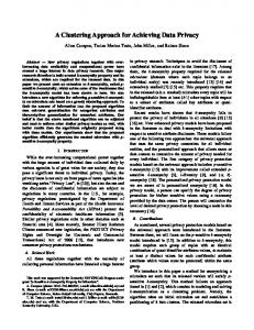
Figure 2 shows the graphical representation of the f(x) function. As it can be seen, the smallest values of the function correspond to clusters that are either unconnected graphs (no edges) or completely connected graphs. The maximum function value corresponds to a cluster that has the number of edges equal to half of the number of all the pairs of nodes in the cluster. A similar analysis, with the same results, can be conducted for the interSIL(cl1, cl2) function, seen as a function of one variable |Ecl1,cl2|, when clusters cl1 and cl2 are fixed. This function has a similar behavior with intraSIL(cl). Namely, minimum is reached when |Ecl1,cl2| is either 0 or the maximum possible value |cl1|⋅|cl2|, and the maximum is reached when |Ecl1,cl2| is equal to |cl1|⋅|cl2| / 2. This analysis suggests that a smaller structural information loss corresponds to clusters in which nodes have similar connectivity properties with one another or, in other words, when cluster’s nodes are either all connected (or unconnected) among them and with the nodes in other clusters. We will use this result in our anonymization algorithm. To normalize the structural information loss, we compute the maximum values for intraSIL(cl) and interSIL(cl1, cl2). As illustrated in Figure 2, the maximum value for intraSIL(cl) is |cl|⋅(|cl| -1) / 4. Similarly, the maximum value for interSIL(cl1, cl2) is |cl1|⋅|cl2| / 2. Using Definition 9, we derive the maximum total structural information loss value as: v
∑ j =1
v
∑ (intraSIL(cl j )) + ∑ ∑ (interSIL(cli , cl j )) . j =1
0
Figure 2. intraSIL as function of number of edges for |cl| fixed
⎛ cl ⎞ + |E | ⋅ ⎛⎜ 1 − E cl ⎜ ⎟ cl ⎜ 2⎟ ⎜ ⎝ ⎠ ⎝
= 2⋅|Ecl| ⋅ ⎜1 − E cl
⎛ cl ⎞ ⎞ ⎜ ⎟⎟ ⎜ 2 ⎟⎟ ⎝ ⎠⎠
Using the first and second derivative function it can easily be determined that the maximum value the function f takes is for x =
each pair of unconnected edges from cluster cl, the probability ⎛ cl ⎞ that someone wrongly labels it as an edge is E cl ⎜ ⎟ . ⎜2⎟ ⎝ ⎠
⎛ cl ⎞ ⎜ ⎟ − Ecl pairs of unconnected nodes in cl, ⎜2⎟ ⎝ ⎠
⎛ f ( x ) = 2 ⋅ x ⋅ ⎜1 − x ⎜ ⎝
⎧⎪ ⎛ cl ⎞⎫⎪ f : ⎨0,1,..., ⎜⎜ ⎟⎟⎬ → R , ⎪⎩ ⎝ 2 ⎠⎪⎭
i =1 j =i +1
We analyze the intraSIL(cl) function for a given fixed cluster cl and a variable number of edges in the cluster, |Ecl|, in other words, we consider intraSIL(cl) a function of a variable |Ecl|. Based on Definition 7, this function is (we use f to denote the function and x the variable number of edges):
=
| cl j | ⋅(| cl j | −1) 4
v
+∑
v
∑
i =1 j =i +1
| cli | ⋅ | cl j |
v v 1 ⎛⎜ v 2 + ⋅ | cl | 2 ∑ j ∑ ∑ | cli | ⋅ | cl j 4 ⎜ j =1 i =1 j =i +1 ⎝
1⎛ v = ⎜ ∑ | cl j 4 ⎜ j =1 ⎝
2
=
2 ⎞ 1 v | ⎟ − ∑ | cl j | = ⎟ 4 j =1 ⎠
⎞ n ⋅ (n − 1) 1 v . | ⎟ − ∑ | cl j | = ⎟ 4 4 j =1 ⎠
The minimum total structural information loss is 0, and it is obtained for a graph with no edges or for a complete graph. Definition 10 (normalized structural information loss): The normalized structural information loss obtained when masking the graph G with n nodes, based on the partition S = {cl1, cl2, … , clv}, denoted by NSIL(G,S), is: NSIL(G,S) =
SIL(G , S )
(n ⋅ (n − 1) 4)
.
The normalized structural information loss is in the range [0, 1].
dist ( X , cl ) =
∑ dist ( X , X j )
X j ∈cl
| cl |
.
We note that both distance measures take values between 0 and 1, and they can be used in the cluster formation process in combination with the normalized generalization information loss. Although this is not formally proved, but shown to be effective in our experiments, by putting together in clusters nodes that are the closest according to the average distance measure, the SaNGreeA algorithm will produce a good masked network, with a small structural information loss.
3.3 The Anonymization Algorithm We put together in clusters, nodes that are as similar as possible, both in terms of their quasi-identifier attribute values, and in terms of their neighborhood structure. By doing that, when collapsing clusters to anonymize the network, the generalization information loss and the structural information loss will both be in an acceptable range.
Algorithm SaNGreeA is Input G = (N, E) – a social network k – as in k-anonymity α and β – user-defined weight parameters
To assess the proximity between nodes with respect to quasiidentifier attributes, we use the normalized generalization information loss. However, the structural information loss cannot be computed during the clusters creation process, as long as the entire partitioning is not known. Therefore, we chose to guide the clustering process using a different measure. This measure quantifies the extent in which the neighborhoods of two nodes are similar with each other, i.e. the nodes present the same connectivity properties, or are connected / disconnected among them and with others in the same way.
i,j=1..v, i≠j; |clj|≥k, j=1..v - a set of clusters that ensures k-anonymity; S = ∅; i = 1; Repeat Xseed = a node with maximum degree from N; cli = {Xseed}; // N keeps track of nodes not yet distributed to clusters N = N - {Xseed}; Repeat X * = argmin α • NGIL(G , S ) + β • dist(X, cl ) ;
To asses the proximity of two nodes neighborhoods, we proceed as follows. Given G = (N, E), assume that nodes in N have a particular order, N = {X 1, X 2, …, X n}. The neighborhood of each node X i can be represented as an n-dimensional boolean vector Bi
(
)
= b1i , b2i ,..., bni , where the jth component of this vector, b ij , is 1 if there is an edge (X i, X j) ∈ E, and 0 otherwise, ∀j = 1,n; j ≠ i. i
We consider the value bi to be undefined, and therefore not equal with 0 or 1. We use a classical distance measure for this type of vectors, the symmetric binary distance [7]. Definition 11 (distance between two nodes): The distance between two nodes (X i and X j) described by their associated ndimensional boolean vectors Bi and Bj is:
dist ( X i , X j ) =
| {l | l = 1..n ∧ l ≠ i, j; bli ≠ blj } | . n−2
We exclude from the two vectors comparison their elements i and j, which are undefined for X i and respectively for X j. As a result, the total number of elements compared is reduced by 2. In the cluster formation process, our greedy approach will select a node to be added to an existing cluster. To assess the structural distance between a node and a cluster we use the following measure. Definition 12 (distance between a node and a cluster): The distance between a node X and a cluster cl is defined as the average distance between X and every node from cl:
Output
v
S = {cl1, cl2,…, clv};
U cl j =
N;
j =1
(
X ∈N
1
1
cli
I cl j = ∅,
i
)
// X* is the node within N (unselected // nodes) that produces the minimal // information loss growth when added to cli // G1 – the subgraph induced by cl ∪ {X} in G; // S1 – a partition with one cluster cl ∪ {X}; cli = cli ∪ {X*}; N = N - {X*}; Until (cli has k elements) or (N == ∅); If (|cli| ≤ k) then DisperseCluster(S, cli); // this happens only for the last cluster Else S = S ∪ {cli}; i++; End If; Until N = ∅; End GreedyPKClustering. Function DisperseCluster(S, cl) For every X ∈ cl do clu = FindBestCluster(X, S); clu = clu ∪ {X}; End For; End DisperseCluster; Function FindBestCluster(X, S) is bestCluster = null; infoLoss = ∞; For every clj ∈ S do If α • NGIL(G1, S1) + β • dist(X, clj)