A CNN-Based Method of Vehicle Detection from Aerial Images ... - MDPI

remote sensing Article

A CNN-Based Method of Vehicle Detection from Aerial Images Using Hard Example Mining Yohei Koga *, Hiroyuki Miyazaki

ID

and Ryosuke Shibasaki

Center for Spatial Information Science (CSIS), University of Tokyo, 5-1-5 Kashiwanoha, Kashiwa-shi, Chiba 2778568, Japan; [email protected] (H.M.); [email protected] (R.S.) * Correspondence: [email protected]; Tel.: +81-4-7136-4290 Received: 31 October 2017; Accepted: 16 January 2018; Published: 18 January 2018

Abstract: Recently, deep learning techniques have had a practical role in vehicle detection. While much effort has been spent on applying deep learning to vehicle detection, the effective use of training data has not been thoroughly studied, although it has great potential for improving training results, especially in cases where the training data are sparse. In this paper, we proposed using hard example mining (HEM) in the training process of a convolutional neural network (CNN) for vehicle detection in aerial images. We applied HEM to stochastic gradient descent (SGD) to choose the most informative training data by calculating the loss values in each batch and employing the examples with the largest losses. We picked 100 out of both 500 and 1000 examples for training in one iteration, and we tested different ratios of positive to negative examples in the training data to evaluate how the balance of positive and negative examples would affect the performance. In any case, our method always outperformed the plain SGD. The experimental results for images from New York showed improved performance over a CNN trained in plain SGD where the F1 score of our method was 0.02 higher. Keywords: vehicle detection; hard example mining; high-resolution; aerial image; satellite image; convolutional neural network (CNN)

1. Introduction Recently, vehicle detection methods have achieved very high performance owing to deep learning techniques; moreover, many more sources of high-resolution aerial and satellite images have become available and affordable. Worldview3 by Digital Globe [1] provides images with a resolution of 0.3 m per pixel, and now many startup companies such as Planet Labs [2] and Black Sky [3] plan to launch small satellites and provide images with a resolution typically around one meter per pixel. For aerial images, in Japan, NTT Geospace [4] provides aerial images that cover 83% of Japan and updates them frequently. In this context, vehicle detection is now being applied to practical issues such as traffic volume surveys and the estimation of economic activity on the ground. Research and development of object detection techniques have significantly progressed in recent years by the advancement of deep learning techniques, in particular, the convolutional neural network (CNN). Region-based CNN (R-CNN) [5] was one of the earliest algorithms to employ CNN for object detection and to demonstrate its great capability. In R-CNN, image regions that possibly contain target objects (called “region proposals”) are chosen by a selective search algorithm [6], and then a CNN algorithm is applied to map target objects in the region proposals. Following R-CNN, many descendants have been proposed. Fast R-CNN [7] and the Spatial Pyramid Pooling network (SPP-net) [8] have improved accuracy and runtime over R-CNN by utilizing an RoI pooling layer—a special case of the spatial pyramid pooling (SPP) layer—and a SPP layer, respectively. They compute a feature map from an entire image only once, and by utilizing the RoI pooling layer or SPP layer,

Remote Sens. 2018, 10, 124; doi:10.3390/rs10010124

www.mdpi.com/journal/remotesensing

Remote Sens. 2018, 10, 124

2 of 21

they classify region proposals by projecting each of them onto that feature map, whereas R-CNN classifies each region proposal independently. However, they also employ a selective search to search region proposals in a target image, which can be time consuming. In Faster R-CNN [9], the selective search is replaced with region proposal networks (RPN). In Faster R-CNN, RPN calculates region proposals from an input image and Fast R-CNN network classifies the region proposals, while these two networks share the same feature map. Faster R-CNN is comprised of only deep learning networks and is 900% faster than Fast R-CNN. However, Faster R-CNN still has room to improve by directly connecting the RPNs and the classifier network. You Look Only Once (YOLO) [10] and Single Shot Multibox Detector (SSD) [11] include such methods, where both the region proposal function and the classification function are embedded in a single network. In these methods, possible object locations (bounding boxes) and class confidences are simultaneously predicted at each pixel of a feature map. These two methods are much faster than Faster R-CNN, while achieving almost the same or even higher accuracy. CNN-based object detection methods, including the ones described above, have been applied to vehicle detection. Chen et al. [12] classified sliding windows, which are bounding boxes densely scattered over an entire image, by a CNN that was enhanced by ramifying the last block of convolutional and pooling layers into three different branches to deal with different scales. They achieved much higher accuracy than those using conventional methods by combining the histogram of oriented gradients (HOG) [13] feature descriptor and the support vector machine (SVM) classifier. Qu et al. [14] employed the Binarized Normed Gradients (BING) [15] algorithm, where gradient features are learnt and used for detecting possible object locations, to obtain region proposals and significantly improved the runtime over [12], while keeping the same level of accuracy as [12]. Faster R-CNN has difficulty when directly applied to vehicle detection in satellite and aerial images, because such images are much larger than natural images and target vehicles are much smaller than objects in natural images. Tang et al. [16] solved this by using enhanced RPNs that utilize a shallow fine feature map and by splitting large target images into small tiles, which are recombined after detection. Similarly, in [17], large images were split into small tiles and fed into YOLO [10] for vehicle detection. While methods such as Faster R-CNN and YOLO are becoming prevalent, the sliding window and region proposal methods are still useful, as they are easy to implement and can adopt any kind of network architecture as a classifier, for instance, a very deep network or novel network architecture. Mundhenk et al. [18] proposed a large open vehicle detection dataset called the “Cars Overhead with Context (COWC)” dataset, and evaluated the usability of context information for vehicle detection. They adopted the sliding window method with a rich model based on GoogLeNet [19] and ResNet [20], which achieved high accuracy on their COWC dataset. While we have shown that vehicle detection methods have improved greatly, the effective use of training data has not been well studied even given its great potential to improve training results, especially in cases where training data are sparse. In practice, data are often sparse in our region of interest and obtaining additional data is usually costly. If we need to train a classifier using only such sparse data, the obtained classifier would be unable to discriminate detailed features. Therefore, it is important to extract as much useful information as possible from the training data. As an alternative, it is also possible to use a classifier trained in a different place where data are abundant. However, the training data acquired from other regions do not necessarily yield better accuracy than the one acquired from the original region. We can improve accuracy by fine-tuning such classifiers with data from our region of interest, but the effective use of training data is also important in these cases. Nevertheless, to our knowledge, this topic does not seem to have been sufficiently studied. Tang et al. [16] employed hard example mining (HEM)—a method to weight more informative samples in learning processes to improve accuracy—by replacing the final classifier part of their Faster R-CNN-based model with a cascade of boosted classifiers of shallow decision trees. In each stage of their Real AdaBoost [21] training, one of the candidate weak classifiers, which best classified the training data, was selected as a part of the final classifier. The misclassified examples were weighted,

Remote Sens. 2018, 10, 124 Remote Sens. 2018, 10, 124

3 of 21 3 of 20

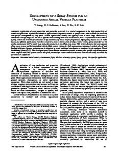
examples. While their attempt succeeded, theystage did not focus on improving the feature learning part and the candidate weak classifiers in the next were imposed on well classifying those weighted in terms of the effective use of training data, which more hard examples. While their attempt succeeded, theyisdid notstraightforward. focus on improving the feature learning In this paper, we proposed the application of HEM to thestraightforward. feature learning process of a CNN part in terms of the effective use of training data, which is more modelInfor vehicle detection from high-resolution aerial images. this paper, we proposed the application of HEM to the feature learning process of a CNN model for vehicle detection from high-resolution aerial images. 2. Methodology 2. Methodology We applied HEM to the stochastic gradient descent (SGD), a commonly used algorithm in deep learning Specifically, we used agradient large batch size, and in each batch, calculated the lossin values We training. applied HEM to the stochastic descent (SGD), a commonly used algorithm deep and employed only examples with the largest loss values for training. In this way, we could always learning training. Specifically, we used a large batch size, and in each batch, calculated the loss values use most informative examples and values to improve accuracy. andthe employed only examples withfor thetraining largest loss for training. In this way, we could always Themost details are as follows. In Section 2.1, weand introduce our basic methodology and its drawbacks. use the informative examples for training to improve accuracy. We first our steps then explain characteristics ofand SGDitswhere there Theintroduce details are as vehicle follows.detection In Section 2.1, and we introduce ourthe basic methodology drawbacks. is room improvement. In Section 2.2,steps we briefly introduce studies ofofHEM explain We first for introduce our vehicle detection and then explainthe therelated characteristics SGD and where there the details our method.InInSection Section 2.3, explain our method of accuracy assessment the is room for of improvement. 2.2, wewe briefly introduce the related studies of HEM and for explain experiments thismethod. paper. In Section 2.3, we explain our method of accuracy assessment for the the details ofinour experiments in this paper. 2.1. Basic Methodology 2.1. Basic Methodology In this paper, we used a simple sliding window method for vehicle detection. Candidate In thisboxes paper,were we used a simple slidingover window method for vehicle detection. Candidate bounding bounding scattered densely an entire image and then those with no existence of boxes were scattered densely over an entire image and then those with no existence of vehicles were vehicles were screened out. HEM was applied to the training of CNN used for the screening. screened out. was applied to the training of CNN used for thesliding screening. Employed Employed CNNHEM architecture was also simple. We employed the simple window methodCNN and architecture was also simple.we Wemainly employed the simple window and CNN architecture, CNN architecture, because focused on the sliding effectiveness of method our HEM method. Our HEM becauseiswe mainly focused on the effectiveness of our HEM method.with OuraHEM is as easily method easily scaled, for instance, by replacing the CNN architecture richermethod one, such the scaled,used for instance, model in [18]. by replacing the CNN architecture with a richer one, such as the model used in [18]. Our HEM method was actually a variant of Online Hard Example Mining (OHEM) [22], which Our HEM designed method was a variant Online Hard Example Mining [22],as which was originally for actually Fast R-CNN, butofrequired modifications to suit (OHEM) our method our was originally designed Fast R-CNN, but required modifications to suit ourdetails method our training training process and thefor Fast R-CNN training process were different. (The areasdescribed in process and the Fast R-CNN training process were different. (The details are described in Section 2.2.) Section 2.2.) 2.1.1. Vehicle Vehicle Detection Detection Methodology Methodology 2.1.1. We structured structured the the algorithm algorithm based based on on the the method methodof of[12]. [12].Figure Figure11shows showsour ourCNN CNNarchitecture. architecture. We

Figure Figure1. 1.The TheCNN CNNarchitecture architectureemployed employedin inthis thisstudy. study.We We introduced introduced batch batch normalization normalization layers layers to to accelerate learning. accelerate learning.

CONV, CONV, BN, BN, ReLU, ReLU, POOL, POOL, FC FC represent represent the the convolutional convolutional layer, layer, batch batch normalization normalization layer, layer, Rectified Linear Unit layer, and fully connected layer, respectively. While we simplified Rectified Linear Unit layer, and fully connected layer, respectively. While we simplified the the CNN CNN architecture process. architecture of of [12], [12], we we added added batch batch normalization normalization [23] [23] layers layers to to accelerate accelerate the the learning learning process. The The window window size size was was set setso sothat thatititfinally finallybecame became50 50pixels pixelsbefore beforeclassification, classification, which which was waslarge large enough to cover a typical vehicle size (see details of our data in Section 3.1). The detailed enough to cover a typical vehicle size (see details of our data in Section 3.1). The detailed vehicle vehicle detection detection steps steps are are as as follows: follows: • • • • •

Threshold a test image by pixel intensity greater than 60 or less than 100 and calculate gradient Threshold a test image by pixel intensity greater than 60 or less than 100 and calculate gradient images, yielding three gradient images (Figure 2). images, yielding three gradient images (Figure 2). Generate sliding windows that overlap each other on half of width and height (Figure 3). Generate sliding windows that overlap each other on half of width and height (Figure 3). Move centers of the windows to geometric centers, which represent possible positions of objects in windows. Geometric centers are calculated as Equation (1):

Remote Sens. 2018, 10, 124

•

4 of 21

Move centers of the windows to geometric centers, which represent possible positions of objects 4 of 20 centers are calculated as Equation (1): 4 of 20

Remote Sens. 2018, 10, 124 windows. Geometric Remotein Sens. 2018, 10, 124

= = gcenter = =S = =

• • •• • • • • •• • •

W H

,

∑ ∑, i

pi,j , Ii,j ,

j

S

(1) (1) (1)

W H

, Ii,j ∑∑ ,

i

j

is a vector which express a pixel position of a geometric center; and are where isa avector vectorwhich whichexpress expressa apixel pixelposition positionofofa geometric a geometric center; and are where where gcenter W and H are the the width andisheight of a window patch, respectively (both are equal to center; the window size); vector the width height a window patch, respectively (both are equal to the window size); vector width andand height of aofwindow (both to the window size); vector pi,j , 1patch, respectively ,1 ; , are is equal a gradient intensity value of a pixel , is a pixel position is a pixel position , ≤ i1≤ W, 1 ≤, 1j ≤ H ); Ii,j; is ,a gradient is a gradient intensity value of a pixel is,,a pixel position intensity value of a pixel i, j 1 i, j ); ( ) ( ( ; and is the sum of the gradient intensity values at all pixels in a window patch (Figure , ; and is the sum of the gradient intensity values at all pixels in a window patch (Figure and S is the sum of the gradient intensity values at all pixels in a window patch (Figure 4a,b). 4a,b). √ 4a,b). Enlarge them by a factor of 2 , and move them to the new geometric centers (Figure 4c,d). Enlarge them by a factor of √2, and move them to the new geometric centers (Figure 4c,d). Discard them unnecessary windows were close We regarded the(Figure windows whose Enlarge by a factor of √2, that and move themto tothe theothers. new geometric centers 4c,d). Discard unnecessary windows that were close to the others. We regarded the windows whose centers were within awindows distance of 0.15 of window as unnecessary (Figure Discard unnecessary that were close to size the others. We regarded the5).windows whose centers were within a distance of 0.15 of window size as unnecessary (Figure 5). centers a distance 0.15 of window size asafter unnecessary (Figure Apply awere CNNwithin to RGB pixels inof the windows remaining the above steps. 5). Apply a CNN to RGB pixels in the windows remaining after the above steps. Apply a CNN to RGB pixels in the windows remaining after the above steps. Examine Examine if if the the windows windows had had overlapping overlapping windows windows with with more more than than 0.5 0.5 of of IoU IoU from from the the highest highest Examine if the windows had overlapping windows with more than 0.5 of IoU from the highest probability of vehicle existence to the lowest. If a window had overlapping windows, probability of vehicle existence to the lowest. If a window had overlapping windows, the the probability ofwindows vehicle were existence to the(this lowest. If anon-maximum-suppression). window had overlapping windows, the overlapping discarded is called overlapping windows were discarded (this is called non-maximum-suppression). overlapping windows were discarded (this is called non-maximum-suppression).

(a) (a)

(b) (b)

(c) (c)

(d) (d)

Figure 2. Original image and calculated gradient images. (a) Original image; (b) gradient of the Figure 2. Original Originalimage imageand and calculated gradient images. (a) Original image; (b) gradient of the Figure calculated gradient images. (a) Original image; (b) ofthresholded the original original2.image; (c) gradient of the image thresholded over 60; (d) gradient of gradient the image original image; (c) gradient of the image thresholded over 60; (d) gradient of the image thresholded image; (c) gradient of the image thresholded over 60; (d) gradient of the image thresholded under 100. under 100. under 100.

Figure 3. How sliding windows are spaced in an image. Figure Figure 3. 3. How Howsliding sliding windows windows are are spaced spaced in in an an image. image.

(a) (a)

(b) (b)

(c) (c)

(d) (d)

Figure 4. An example of a sliding window move. (a) An initial window; (b) moved to its geometric Figure 4. An example of a sliding window move. (a) An initial window; (b) moved to its geometric center; (c) enlarged; (d) moved to its new geometric center. center; (c) enlarged; (d) moved to its new geometric center.

Remote Sens. 2018, 10, 124

5 of 21

Figure 3. How sliding windows are spaced in an image.

(a)

(b)

(c)

(d)

Figure 4. 4. An An example example of of aa sliding sliding window window move. move. (a) (a) An An initial initial window; window; (b) (b) moved moved to to its its geometric geometric Figure center; (c) enlarged; (d) moved to its new geometric center. center; (c) enlarged; (d) moved to its new geometric center.

Remote Sens. 2018, 10, 124

5 of 20

Figure 5. How to discard unnecessary windows. Figure 5. How to discard unnecessary windows.

We did not use any meta information such as shadow directions. In terms of sliding window We did use anythe meta information as shadow directions. InAppendix terms of sliding window accuracy, wenot evaluated negative impactsuch of clutter and shadows in the A. accuracy, we evaluated the negative impact of clutter and shadows in the Appendix A. 2.1.2. Stochastic Gradient Descent (SGD) and Room for Improvement 2.1.2. Stochastic Gradient Descent (SGD) and Room for Improvement SGD is an algorithm for optimizing parameters in machine learning that is commonly used in SGD is an algorithm for optimizing parameters in machine learning that is commonly used in deep learning. First, we explain gradient descent (also called batch gradient descent) on which SGD deep learning. First, we explain gradient descent (also called batch gradient descent) on which SGD is is based. In machine learning, parameters are optimized by minimizing the objective function (also based. In machine learning, parameters are optimized by minimizing the objective function (also often often called the loss function). In gradient descent, a parameter is updated by called the loss function). In gradient descent, a parameter is updated by θ ← θ-α∇θ J(θ) (2) θ ← θ − α∇ θ J (θ ) (2) where θ is the parameter, α is the learning rate, J is the objective function, and its derivative θ J θ is called In gradient descent, rate, gradients areobjective calculated over alland examples in the training where θ isthe thegradient. parameter, α is the learning J is the function, its derivative ∇θ J (θ ) data andthe used to update θ [24,25].descent, This is repeated until is convergence. However, is called gradient. In gradient gradients arethere calculated over all examples inthis the becomes training inefficient or infeasible theThis number of training [24,25]. Hence in SGD, a small data and used to update when θ [24,25]. is repeated until data thereisis huge convergence. However, this becomes number ofor examples—called minibatch—are sampleddata from entire training dataset and used for inefficient infeasible whenathe number of training isthe huge [24,25]. Hence in SGD, a small training. Sampling a minibatch is random as giving training data in some meaningful order can bias number of examples—called a minibatch—are sampled from the entire training dataset and used for gradientsSampling and lead atominibatch poor convergence [25]. all of theintraining data are first shuffled [25] training. is random as Specifically, giving training data some meaningful order can bias and partitioned (usually equally) into minibatches, then each is processed for shuffled optimization gradients and lead to poor convergence [25]. Specifically, all ofminibatch the training data are first [25] in order. Strictly speaking, this should be called minibatch gradient descent, and SGD originally and partitioned (usually equally) into minibatches, then each minibatch is processed for optimization meant only a singlethis training example [24]; however, we usedescent, this term it is originally commonly used in order.using Strictly speaking, should be called minibatch gradient andasSGD meant in a deep context.example This is based on the assumption approximates the using only learning a single training [24]; however, we use thisthat termeach as it minibatch is commonly used in a deep entire training dataset well [24]. One minibatch process is called an iteration, and processing the learning context. This is based on the assumption that each minibatch approximates the entire training entire dataset is called an epoch. Training continues epochsand until convergence. dataset well [24]. One minibatch process is called anover iteration, processing the entire dataset is Now let the weight variables of our model be W, minibatch input data be X, labels (the numbers called an epoch. Training continues over epochs until convergence. which express the classes) of X be T, and loss function be L(W, X, T). Note that if x and t are single Now let the weight variables of our model be W, minibatch input data be X, labels (the numbers examples of Xthe andclasses) T, respectively, X, T)function must bebethe summation of all x, t) t[26]. Given which express of X be T,L(W, and loss L(W, X, T). Note thatL(W, if x and are single concrete input X and labels T, we can regard the X and T as the coefficients of L. Therefore, L is examples of X and T, respectively, L(W, X, T) must be the summation of all L(W, x, t) [26]. Given regarded as a function of W. We can interpret Equation (2) as follows: W ← W-α∇W L(W, X, T)

(3)

This equation updates W so that the loss function becomes smaller. As a consequence, the model becomes able to classify input well. The gradient of each weight variable is calculated by propagating derivatives from the tail to the head of the model based on the chain rule, which is called back propagation [26]. Conversely, calculating output or loss function of a model when given an input is called forward propagation.

Remote Sens. 2018, 10, 124

6 of 21

concrete input X and labels T, we can regard the X and T as the coefficients of L. Therefore, L is regarded as a function of W. We can interpret Equation (2) as follows: W ← W − α∇W L(W, X, T)

(3)

This equation updates W so that the loss function becomes smaller. As a consequence, the model becomes able to classify input well. The gradient of each weight variable is calculated by propagating derivatives from the tail to the head of the model based on the chain rule, which is called back propagation [26]. Conversely, calculating output or loss function of a model when given an input is called forward propagation. As training progresses, most of the loss values in a minibatch become very small. However, there are still some examples where the loss values are relatively large. We can find analogs of these in the test results. When we conduct vehicle detection with a trained classifier, many of the bounding boxes are classified correctly, but still there can be some that are misclassified. These are sometimes called hard examples. For instance, they may have vehicle-like features that are difficult to discriminate (see Figure 6 for examples). Remote Sens. 2018, 10, 124 6 of 20

Figure 6. Instances of hard example patches. Figure 6. Instances of hard example patches.

Such examples are likely to give clues to discriminating confusing features; therefore, utilizing Such examples are likely to give discriminating confusing they features; therefore, utilizing them in training processes seems to clues yield to better accuracy. However, would not sufficiently them in training processes seems to yield better accuracy. However, they would not sufficiently contribute to learning in an ordinary SGD. As described above, most loss values in a minibatch contribute to learning an ordinary SGD. As described above, most loss in a minibatch become become very small as in training progresses, and gradients calculated overvalues a minibatch are aggregated very small as training progresses, gradientsexamples calculated a minibatch arelarge aggregated and averaged. This means the fewand informative areover diluted by another part ofand the averaged. This means the few informative examples are diluted by another large part of the minibatch minibatch that do not contribute to improving accuracy. In this way, hard examples contribute little that do not contribute tothis, improving accuracy. In thisthe way, hard examples contribute little to learning. to learning. To address we needed to choose informative examples and preferentially use To address this, we needed to choose the informative examples and preferentially use them for training, them for training, which is called hard example mining. which is called hard example mining. 2.2. Hard Example Mining (HEM) in SGD Training 2.2. Hard Example Mining (HEM) in SGD Training In HEM, hard examples, which are difficult to classify correctly, are weighted more than other In HEM, hard examples, which are difficult to classify correctly, are weighted more than other examples for training. Typically, hard examples are selected if they are difficult to correctly classify examples for training. Typically, hard examples are selected if they are difficult to correctly classify for for a current classifier. HEM has been conventionally used in machine learning, e.g., for SVM training. a current classifier. HEM has been conventionally used in machine learning, e.g., for SVM training. For pedestrian detection, Dalal and Triggs [13] searched hard examples with a preliminarily trained For pedestrian detection, Dalal and Triggs [13] searched hard examples with a preliminarily trained detector and additionally used them for training a final detector. Felzenszwalb et al. [27] iteratively detector and additionally used them for training a final detector. Felzenszwalb et al. [27] iteratively updated the training data subset by discarding easy examples that were correctly classified beyond updated the training data subset by discarding easy examples that were correctly classified beyond the current classifier’s margin and adding hard examples that violated the current classifier’s margin. the current classifier’s margin and adding hard examples that violated the current classifier’s margin. Using a non-SVM method, Tang et al. [16] adopted a cascade of boosted classifiers of shallow decision Using a non-SVM method, Tang et al. [16] adopted a cascade of boosted classifiers of shallow decision trees as the final classification part of their vehicle detection method. In each stage of their Real trees as the final classification part of their vehicle detection method. In each stage of their Real AdaBoost [21] training, a weak classifier that best classified the training data was selected as part of AdaBoost [21] training, a weak classifier that best classified the training data was selected as part of the final classifier. The misclassified examples were weighted, and the candidate weak classifiers in the final classifier. The misclassified examples were weighted, and the candidate weak classifiers in the next stage were imposed on well classifying those weighted hard examples. the next stage were imposed on well classifying those weighted hard examples. In object detection by deep learning, a heuristic method has been previously used. In Fast RCNN [7] and SPP-net [8], when sampling reference background patches for training data, if the IoU between a background patch and a foreground patch is lower than 0.1, the sampled background patch is excluded from training data, because the patch is not a hard example given that the patch is easily classified to the background patch. If a background patch overlaps a foreground patch in a much portion, such as cases where the IoU is much higher than 0.1, the patch is chosen as training data because the patch is useful as a hard example as the background patch is likely to be confused

Remote Sens. 2018, 10, 124

7 of 21

In object detection by deep learning, a heuristic method has been previously used. In Fast R-CNN [7] and SPP-net [8], when sampling reference background patches for training data, if the IoU between a background patch and a foreground patch is lower than 0.1, the sampled background patch is excluded from training data, because the patch is not a hard example given that the patch is easily classified to the background patch. If a background patch overlaps a foreground patch in a much portion, such as cases where the IoU is much higher than 0.1, the patch is chosen as training data because the patch is useful as a hard example as the background patch is likely to be confused with the foreground. This improves accuracy to some extent but is suboptimal, as there could be some hard examples in the excluded patches. To address this, Shrivastava et al. [22] proposed Online Hard Example Mining (OHEM). In OHEM, the loss values of all region proposals in an image are calculated by the current classifier and only examples with the largest losses are picked for a minibatch. OHEM further improved accuracy over the heuristic method. However, we could not directly apply OHEM to our method because OHEM is designed for Fast R-CNN, a training process that is different from ours. In Fast R-CNN training, an image is randomly selected from all training images, region proposals are calculated in the image, and 64 of them are selected for a minibatch (in practice, their minibatch consists of 128 examples from two images). As Fast R-CNN employs RoI pooling—in which the feature map is calculated from an entire image only once and10, region Remote Sens. 2018, 124 proposals are classified by projecting each of them onto the feature map—this 7 of 20 image-wise training is effective. OHEM replaces the selection of region proposals for a minibatch and also benefits RoI pooling terms ofineffective Meanwhile, in our algorithm minibatch and alsofrom benefits from RoIinpooling terms ofcomputation. effective computation. Meanwhile, in our proposed proposed in Sectionin 2.1.1., we 2.1.1., preliminarily extractedextracted patches from all training sampled algorithm Section we preliminarily patches from all images, training and images, and minibatches randomly from them. Wethem. needed modifytoOHEM our training sampled minibatches randomly from Weto needed modifytoOHEM to our procedure. training procedure. Here Herewe weexplain explainour ourmethod methodin indetail. detail.Figure Figure77shows showsan anoverview overviewof ofthe the algorithm. algorithm.

Figure7.7.Algorithm Algorithmoverview. overview.Loss Lossvalues valuesare arecalculated calculatedin ineach eachcheckbatch checkbatchand andonly onlyexamples exampleswith with Figure thelargest largestlosses lossesare areused usedfor fortraining. training. the

First, theentire entiretraining trainingdataset dataset and partitioned it into batches of ncheck. size ncheck. We First, we we shuffled shuffled the and partitioned it into batches of size We called called each batch a checkbatch, and ncheck is the number of examples where the loss values are each batch a checkbatch, and ncheck is the number of examples where the loss values are checked in checked in one iteration. Then, we processed each checkbatch one by one. In each checkbatch, we one iteration. Then, we processed each checkbatch one by one. In each checkbatch, we calculated calculated the loss withclassifier, a currentsorted classifier, sorted byinloss values inorder, descending the loss values withvalues a current examples byexamples loss values descending picked order, picked nlearn examples with the largest losses, and used them for training to update theclassifier; current nlearn examples with the largest losses, and used them for training to update the current classifier; nlearn is theofnumber ofthat examples that are actually used for This repeated process was nlearn is the number examples are actually used for training. Thistraining. process was over repeated over epochs until convergence. While ncheck was larger than nlearn, the ratio can be decided epochs until convergence. While ncheck was larger than nlearn, the ratio can be decided arbitrarily. arbitrarily. The is algorithm is summarized in Algorithm 1. The algorithm summarized in Algorithm 1. Algorithm 1: Hard example mining in SGD Input: Training dataset D, nlearn, ncheck, epochs, classifier Output: Trained classifier Initialize variables of For e = 1 to epochs: Shuffle D Split D into size(D)/ncheck checkbatches For each checkbatch: Compute loss values of examples in the checkbatch by Sort the examples in the checkbatch by loss values in descending order Train using the top nlearn examples

Remote Sens. 2018, 10, 124

8 of 21

Algorithm 1: Hard example mining in SGD Input: Training dataset D, nlearn, ncheck, epochs, classifier f Output: Trained classifier f Initialize variables of f For e = 1 to epochs: Shuffle D Split D into size(D)/ncheck checkbatches For each checkbatch: Compute loss values of examples in the checkbatch by f Sort the examples in the checkbatch by loss values in descending order Train f using the top nlearn examples

In this way, for training, only the examples with the largest losses are always used, which are the most informative ones. We expect our method to promote the learning of finer features, and it should also find the optimal balance of positive and negative examples in the training examples, the same as in [22]. Recall that SGD is based on the assumption that each minibatch approximates the entire training dataset well, as described in Section 2.1.2. From this viewpoint, we can say that our proposed method approximates checking the loss values of all the training data and only selected the most informative examples for training in one iteration. In plain SGD, the entire training dataset is split into minibatches and each minibatch is used for training, which means all the examples in the training data are used for training. However, in the proposed method, we only used a part of the examples for training in one epoch because we selected only the examples with the largest loss values. Therefore, we compared plain SGD and the proposed method in the same iteration, not in the same literal epoch. Here, we also explain the implementation details. As is common practice, we adopted softmax cross entropy as the loss function as defined as follows: loss(y, t) = −

1 N

N

C

∑ ∑ tnc ln ync ,

(4)

n =1 c =1

where y is the softmax output; N is minibatch size; C is the number of classes; and t is a label. Only one true label among C is 1 and the others are 0. According to this equation, when we want to sort examples of a minibatch by loss values, we only need to check the prediction results, i.e., the last activation of the model corresponding to the true class. There are two ways to implement the proposed method. The first is to calculate all of the loss values in a checkbatch, set the loss values to zeros (except the largest ones), and train. The second is to preliminarily select examples with the worst prediction results in a checkbatch, calculate their loss values, and train. We adopted the second procedure in this paper, mainly because we introduced batch normalization layers [23] into our CNN, as mentioned in Section 2.1.1. Batch normalization normalizes a minibatch so that the mean and the variance of the minibatch become 0 and 1, respectively. If the first implementation is adopted, after examples with the largest losses in a checkbatch are selected, the batch normalization needs to be re-calculated, because the minibatch statistics are generally changed. However, we cannot recalculate the batch normalization by linear transformation of the previous forward propagation result because our CNN also has non-linear ReLU layers as mentioned in Section 2.1.1. Therefore, there is a need to recalculate the loss values of the selected examples after all. For this reason, we adopted the second implementation. Batch normalization has a training mode and a testing mode, and different statistics are used to normalize a minibatch in each mode. In the training mode, it uses the statistics of the current minibatch, and in testing mode it uses the statistics of all the data that have been used for training. We used the testing mode in the loss checking process, because our idea was to use examples that were difficult to classify by the current classifier.

Remote Sens. 2018, 10, 124

9 of 21

2.3. Accuracy Assesment 2.3.1. Vehicle Detection Criteria We adopted the same criteria as [12]. When a window was detected as containing vehicles, if the distance of centers between it and any groundtruth was smaller than 0.45 of the window size, it was judged as true positive (TP), otherwise it was a false positive (FP). A groundtruth was judged to be detected if it had at least one corresponding TP. In these criteria, it is possible to have multiple TPs for one vehicle, which are redundant except for one TP. One TP is allowed to detect only one vehicle. 2.3.2. Quantitative Measure We calculated the recall rate (RR), precision rate (PR), and false alarm rate (FAR) as per [12,14]. We also calculated the F1 scores by using the obtained RR and PR scores. detected groundtruths groundtruths detected groundtruths PR = detected windows false positives FAR = groundtruths 2 × PR × RR F1 = PR + RR

RR =

3. Experiment and Results Remote Sens. 2018, 10, 124

9 of 20

We evaluated the performance of our method by comparing it with plain SGD training (hereinafter called the and normal First, we trained CNNs the classifiers. normal and and then methods, thenmethod). conducted vehicle detection withby those Anproposed overviewmethods, of the experiment conducted vehicle detection with those classifiers. An overview of the experiment is shown in Figure 8. is shown in Figure 8.

Figure Figure 8. 8. Experiment Experiment overview. overview.

We used sparse training data as explained in Sections 3.1 and 3.2. We conducted preliminary We used sparse training data as explained in Sections 3.1 and 3.2. We conducted preliminary experiments using the normal method and found that it still had room for improvement, because the experiments using the normal method and found that it still had room for improvement, because the FAR in the result was high. We aimed to reduce false positives and improve the accuracy by using FAR in the result was high. We aimed to reduce false positives and improve the accuracy by using the the proposed method, which was the first motivation of this paper. proposed method, which was the first motivation of this paper. 3.1. Training and Test Images 3.1. Training and Test Images We downloaded aerial ortho images of New York from the U.S. Geological Survey (USGS), cut We downloaded aerial ortho images of New York from the U.S. Geological Survey (USGS), cut out areas of harbors and malls, and used them for training and testing. The pixel size of all images out areas of harbors and malls, and used them for training and testing. The pixel size of all images was was 0.15 m. Table 1 shows the images and their attributes. The train_2 image was taken in the spring 0.15 m. Table 1 shows the images and their attributes. The train_2 image was taken in the spring of of 2013, and the rest was taken in April–May of 2014. These were the only images used in this paper. 2013, and the rest was taken in April–May of 2014. These were the only images used in this paper. Table 1. Training and test images. Training Images

Test Images

Training Test Images 3.1. Training and Test Images 3.1. 3.1.3.1. Training Training and andand Test Test Images Images downloaded aerial ortho images of York from U.S. Geological Survey (USGS), We downloaded aerial ortho images ofNew New York from the U.S. Geological Survey (USGS), cut We WeWe downloaded downloaded aerial aerial ortho ortho images images of of New New York York from from the thethe U.S. U.S. Geological Geological Survey Survey (USGS), (USGS), cut cutcut areas of and malls, and used them training and testing. The pixel size of images out areas ofharbors harbors and malls, and used them for training and testing. The pixel size ofall all images out outout areas areas of of harbors harbors and and malls, malls, and and used used them them for forfor training training and and testing. testing. The The pixel pixel size size of of all all images images Remote Sens. 2018, 10, 124 10 of 21 was 0.15 Table 11shows images and their attributes. The train_2 image was taken in spring was 0.15 m. Table shows the images and their attributes. The train_2 image was taken inthe the spring was was 0.15 0.15 m. m.m. Table Table 11 shows shows the thethe images images and and their their attributes. attributes. The The train_2 train_2 image image was was taken taken in in the the spring spring of and rest was taken in of These were only images used in paper. of2013, 2013, and the rest was taken inApril–May April–May of2014. 2014. These were the only images used inthis this paper. of of 2013, 2013, and and the thethe rest rest was was taken taken in in April–May April–May of of 2014. 2014. These These were were the thethe only only images images used used in in this this paper. paper. Table 1. Training and test images. Table 1.1.Training and images. Table Training and test images. Table Table 1. 1. Training Training and and test testtest images. images. Training Images Training Images Training Images Training Training Images Images

Name Name Name Name Name City City City City City Feature Feature Feature Feature Feature Area Area Area Area Area Vehicle Vehicle Vehicle Vehicle Vehicle

train_1 train_2 train_1 train_2 train_1 train_1 train_2 train_2 train_1 train_2 New York New York New New York York New York Harbor Mall Harbor Mall Harbor Harbor Mall Mall Harbor Mall 2 2 2 2 22 2 2 22km km 0.08 km 0.16 km 0.08 0.16 km kmkm 0.08 0.08 km km 0.16 0.16 0.16 0.08 km 821 821 687 821 687 687687 821 821

Test Images Test Images Test Images Test Test Images Images

test_1 test_1 test_1 test_1 test_1

test_2 test_2 test_2 test_2 test_2 New York New York New New York York New York Harbor Mall Harbor Mall Harbor Harbor Mall Mall Harbor Mall 2 22 2 2 2 2 22km 0.16 0.12 0.16 km 0.12 0.16 0.16 km kmkm 0.12 0.12 km km2km 0.16 km 0.12 km 806 510 806 510 806 806806 510510

Data Preparation 3.2. Data Preparation 3.2. 3.2.3.2. Data Data Preparation Preparation prepared groundtruth maps of images described in choosing aapixel We prepared groundtruth maps ofall all the images described inSection Section 3.1 by choosing pixel in We WeWe prepared prepared groundtruth groundtruth maps maps of of all all the thethe images images described described in in Section Section 3.1 3.13.1 by byby choosing choosing aa pixel pixel in in in prepared center of vehicle Then generated training dataset patches from the center ofeach each vehicle byhand. hand. Then we generated the training dataset byextracting extracting patches from the thethe center center of ofeach each vehicle vehicle by byby hand. hand. Then Then we we generated generated the thethe training training dataset dataset by byby extracting extracting patches patches from from Then wewe generated training training images. positive examples, first extracted bounding boxes around dots in the training images. For positive examples, we first extracted bounding boxes around the dots inthe the the thethe training training images. For ForFor positive positive examples, examples, we wewe first first extracted extracted bounding bounding boxes boxes around around the thethe dots dots in in the the images. groundtruth maps as groundtruth patches. The window size was 50 pixels, which was designed groundtruth maps as groundtruth patches. The window size was 50 pixels, which was designed to groundtruth groundtruth maps maps as as groundtruth The window window size was was 50 50 pixels, groundtruth patches. patches. The windowsize pixels, which which was was designed designed to to to well cover typical size of increase variance of positive examples, generated well cover the typical size ofvehicles. vehicles. To increase the variance ofthe the positive examples, we generated well cover the typical typical size size of ofvehicles. vehicles. To ToTo increase increase the thethe variance variance of ofthe the positive positive examples, examples, we wewe generated generated well cover thethe ◦ ◦ duplications of groundtruth patch at angles from 9° to 90° in increments 10rotated rotated duplications ofeach each groundtruth patch atrotation rotation angles from 9° to 90° in increments of 10 1010 rotated rotated duplications duplications of of each each groundtruth groundtruth patch patch at at rotation rotation angles angles from from 9° 9° to to 90° 90° in in increments increments of of of 9 90 ◦ This isiscalled data augmentation. Then, negative examples, extracted background patches 9°. This called data augmentation. Then, for negative examples, we extracted background patches 9°. 9°. This This is is called called data data augmentation. augmentation. Then, Then, for forfor negative negative examples, examples, we wewe extracted extracted background background patches patches 9 .9°. This Then, randomly where IoU between aacandidate patch and any groundtruth was lower than These randomly where the IoU between candidate patch and any groundtruth was lower than 0.4. These randomly randomly where the IoU between aa candidate patch and any groundtruth was lower than 0.4. These where thethe IoU between candidate patch and any groundtruth was lower than 0.4.0.4. These types of commonly used. The authors in [14] used similar methods for data preparation. types ofmethods methods are commonly used. The authors in [14] used similar methods for data preparation. types types of of methods methods are areare commonly commonly used. used. The The authors authors in in [14] [14] used used similar similar methods methods for for data data preparation. preparation. The authors in [14] used similar methods for data preparation. Finally, patches were resized to which was input size of CNN. Finally, all patches were resized to48 48by by 48pixels, pixels, which was the input size ofour our CNN. Finally, Finally, all allall patches patches were were resized resized to 48 48 by 4848 pixels, which was thethe input size ofour our CNN. CNN. Finally, to by 48 pixels, which was the input size of CNN. We generated five different training datasets. The groundtruth patches were always the same, whereas the amounts of sampled background patches were different. The ratios of background patches to groundtruth patches (without the augmented ones) were 100:1, 200:1, 300:1, 400:1, and 500:1 (hereinafter called ×100, ×200, ×300, ×400, and ×500), respectively. For instance, in the case of ×100, the ratio of positive examples (including augmented ones) to negative examples was 11:100. We used them, because the balance of positive and negative examples in the training data generally affects the result, and we aimed to evaluate this effect. As the background area is generally larger than the foreground area in an image, it is common to use more negative examples than positive examples in the training data for better accuracy [1,7,8,11,14]. This is more conspicuous in the case of vehicle detection, because vehicles are small objects. Taking these into account, we began the ratio of positive to negative examples from 11:100. In each training dataset, we randomly selected one-tenth of the dataset and used it as a fixed hold-out validation dataset. During training, we calculated the loss and accuracy on this validation dataset in every epoch, which was its only use. 3.3. Experiment We trained classifiers with the normal method and our proposed method. In the proposed method, we used two ncheck values of 500 and 1000 (hereinafter called HEM500 and HEM1000, respectively) to evaluate the effect of this parameter. Due to our limited computing resources, we could test only these cases. For each training method, we used the ×100, ×200, ×300, ×400, and ×500 datasets as described in Section 3.2. After training, we conducted vehicle detection tests with these trained classifiers. Table 2 shows all the experimental conditions, which are combinations of the training method and the background patch amount.

Remote Sens. 2018, 10, 124

11 of 21

Table 2. Experimental conditions, which are combinations of the training method and the background patch amount. Each pair in parentheses expresses one experimental condition. Training Method

BG patch amount

×100 ×200 ×300 ×400 ×500

Normal

HEM500

HEM1000

(×100, Normal) (×200, Normal) (×300, Normal) (×400, Normal) (×500, Normal)

(×100, HEM500) (×200, HEM500) (×300, HEM500) (×400, HEM500) (×500, HEM500)

(×100, HEM1000) (×200, HEM1000) (×300, HEM1000) (×400, HEM1000) (×500, HEM1000)

Since we trained the CNN classifiers from scratch and initialized the weight variables randomly, the performances of the trained classifiers were slightly different. To mitigate these fluctuations, we repeated all experiments under each condition 10 times and averaged the results. The standard deviations and standard errors are shown in the result tables. 3.4. Training Results We initialized the CNN weight variables at random. We used the Adam solver [28], and the training iterations were equivalent to 100 epochs in the normal method. (e.g., 500 epochs when ncheck was five times larger than nlearn). The batch size for learning (i.e., nlearn) was constantly 100. These were decided empirically based on preliminary experiments. In every epoch during training, the mean loss and mean accuracy were calculated for the training and validation datasets. As the shapes of all of the graphs were similar for the different conditions, we present only one example. Figure 9 shows the training curves where the background patch amount was ×200 (one of the results of repeated experiments). In Figure 9, all methods seem to have sufficiently converged. For training loss and accuracy, the fluctuations of the proposed method were larger than the normal method. This seems natural because in every iteration, the CNN is updated and used to calculate loss values and select training examples, which means that the criteria of selecting training examples changed in every iteration. Figure 10 shows the moving average of Figure 9d, which aimed to show the convergence trend more clearly. In Figure 10, we averaged about 6350 iterations, which corresponded to two epochs of the normal method. As Figure 10 shows, while the accuracy in the normal method still improved slightly toward the last epochs, it improved much faster in the proposed method. This means that the proposed method markedly accelerated convergence. In addition, the curve of HEM1000 seems to have converged slightly earlier than that of HEM500. This indicates that the larger ncheck accelerated convergence more. To evaluate the training results, we compared the final values of validation loss and validation accuracy under different conditions. To mitigate fluctuations, we calculated the moving average of iterations corresponding to 10 epochs of the normal method and then averaged the repeated experiments. Table 3 shows the statistics, which include the standard deviations and standard errors. While validation losses were not necessarily smaller in the proposed method than in the normal method, validation accuracies were always higher in the proposed method than in the normal method, which can be said explicitly according to the standard errors. Although the main purpose of this validation was to check the overfitting occurrence, this result is evidence that the proposed method yielded better generalization. When we compared the validation accuracies of HEM500 and HEM1000, we could not see a significant difference. Note that this accuracy calculation included classifying the background patches. The performance of our system in terms of vehicle detection is evaluated in Section 3.5.

Remote Sens. 2018, Remote Sens. 2018, 10,10, 124124

11 11 of of 20 20

theconvergence convergencetrend trendmore moreclearly. clearly.InInFigure Figure10,10,weweaveraged averagedabout about6350 6350iterations, iterations,which which the 12 of 21 corresponded two epochs the normal method. corresponded toto two epochs ofof the normal method.

Remote Sens. 2018, 10, 124

(a)(a)

(b)(b)

(c)(c)

(d)(d)

Figure 9. Training curve example. The background patch amount was ×200 in this case. Training Figure Training curve example. The background patch amount was in this this case. (a)(a) Training Figure 9.9.Training curve example. The background patch amount was ××200 200 in case. (a) Training loss; training Accuracy; validation loss; and validation accuracy. loss; (b)(b) training Accuracy; (c)(c) validation loss; and (d)(d) validation accuracy. loss; (b) training Accuracy; (c) validation loss; and (d) validation accuracy.

Figure Moving average of Figure Figure 10.10. Moving average ofFigure Figure 9d.9d. Figure 10. Moving average of 9d.

Figure shows, while the accuracy the normal method still improved slightly toward the AsAs Figure 1010 shows, while the accuracy inin the normal method still improved slightly toward the last epochs, improved much faster the proposed method. This means that the proposed method last epochs, it it improved much faster inin the proposed method. This means that the proposed method markedly accelerated convergence. In addition, the curve of HEM1000 seems to have converged markedly accelerated convergence. In addition, the curve of HEM1000 seems to have converged slightlyearlier earlierthan thanthat thatofofHEM500. HEM500.This Thisindicates indicatesthat thatthe thelarger largerncheck ncheckaccelerated acceleratedconvergence convergence slightly more. more. evaluate the training results, compared the final values validation loss and validation ToTo evaluate the training results, wewe compared the final values ofof validation loss and validation accuracy under different conditions. mitigate fluctuations, calculated the moving average accuracy under different conditions. ToTo mitigate fluctuations, wewe calculated the moving average ofof iterations corresponding to 10 epochs of the normal method and then averaged the repeated iterations corresponding to 10 epochs of the normal method and then averaged the repeated

method, validation accuracies were always higher in the proposed method than in the normal method, which can be said explicitly according to the standard errors. Although the main purpose of this validation was to check the overfitting occurrence, this result is evidence that the proposed method yielded better generalization. When we compared the validation accuracies of HEM500 and HEM1000, we10,could Remote Sens. 2018, 124 not see a significant difference. Note that this accuracy calculation included 13 of 21 classifying the background patches. The performance of our system in terms of vehicle detection is evaluated in Section 3.5. Table 3. Statistics of the last values of validation loss and validation accuracy. We calculated the moving average graphs and averaged the repeated experiments. Here we emphasized the best accuracy among Table 3. Statistics of the last values of validation loss and validation accuracy. We calculated the methods in bold font. moving average graphs and averaged the repeated experiments. Here we emphasized the best accuracy among methods in bold font. Last Validation Loss Last Validation Accuracy Training BG Patch Method Last Validation Loss Average STDDEV STDERR AverageLast Validation STDDEV Accuracy STDERR BG Patch Training Method Average STDDEV STDERR Average STDDEV STDERR Normal 0.0031 0.0006 0.0002 99.932% 0.013% 0.004% Normal 0.0031 0.0006 0.0002 99.932% 0.013% 0.004% HEM500 0.0030 0.0005 0.0002 99.950% 0.005% 0.002% ×100 0.0030 99.950% HEM500 0.0005 0.0002 0.005% 0.002% ×100 HEM1000 0.0036 0.0008 0.0003 99.949% 0.014% 0.005% HEM1000 0.0036 0.0008 0.0003 99.949% 0.014% 0.005% Normal 0.0016 0.0004 0.0001 99.957% 0.008% 0.003% Normal 0.0016 0.0004 0.0001 99.957% 0.008% 0.003% HEM500 0.0015 0.0005 0.0002 99.973% 0.006% 0.002% ×200 99.973% HEM500 0.0015 0.0005 0.0002 0.006% 0.002% ×200 HEM1000 0.0013 0.0002 0.0001 99.973% 0.002% 0.001% 0.0013 99.973% HEM1000 0.0002 0.0001 0.002% 0.001% Normal 0.002% Normal 0.0019 0.00190.0003 0.00030.0001 0.000199.963% 99.963% 0.007% 0.007% 0.002% HEM500 0.0022 0.0005 0.0002 99.974% 0.006% 0.002% ×300 99.974% HEM500 0.0022 0.0005 0.0002 0.006% 0.002% ×300 HEM1000 0.0022 0.0004 0.0001 99.973% 0.003% 0.001% HEM1000 0.0022 0.0004 0.0001 99.973% 0.003% 0.001% Normal 0.001% Normal 0.0016 0.00160.0003 0.00030.0001 0.000199.969% 99.969% 0.004% 0.004% 0.001% HEM500 0.001% ××400 400 HEM500 0.0017 0.00170.0002 0.00020.0001 0.000199.978% 99.978% 0.003% 0.003% 0.001% HEM1000 0.0016 0.0003 0.0001 99.981% 0.003% 0.001% 0.0016 99.981% HEM1000 0.0003 0.0001 0.003% 0.001% Normal 0.0011 0.0002 0.0001 99.978% 0.003% 0.001% Normal 0.0011 0.0002 0.0001 99.978% 0.003% 0.001% HEM500 0.001% ××500 500 99.986% 0.003% HEM500 0.0010 0.00100.0002 0.00020.0001 0.000199.986% 0.003% 0.001% HEM1000 0.001% 99.986% 0.002% HEM1000 0.0011 0.00110.0002 0.00020.0001 0.000199.986% 0.002% 0.001%

3.5. 3.5.Vehicle VehicleDetection DetectionResults Results We Weconducted conductedvehicle vehicledetection detectionusing usingthe themethod methoddescribed describedininSection Section2.1.1 2.1.1and andthe thetest testimages images described in Section 3.1. Results of repeated experiments were averaged. described in Section 3.1. Results of repeated experiments were averaged. Figure Figure11 11shows showsthe theF1-measure F1-measureresults resultsand andTable Table44shows showsthe thestatistics statisticsofofall allquantitative quantitative measures, measures,which whichinclude includethe thestandard standarddeviations deviationsand andstandard standarderrors. errors.

Figure 11. F1 scores in each condition. Our proposed method improved the scores in all cases over Figure 11. F1 scores in each condition. Our proposed method improved the scores in all cases over the the normal method. normal method.

In terms of F1 scores, while almost all of the standard errors were smaller than 0.01, the proposed method improved the scores by over 0.02 when compared to the normal method in most cases, which proved the effectiveness of our proposed method. Moreover, because the standard deviations of all methods were not very different, we can say our proposed method worked stably.

Remote Sens. 2018, 10, 124

14 of 21

Table 4. Statistics of all quantitative measures. Here we emphasized the best accuracy among methods in bold font. FAR

PR

RR

F1

Training Method

Avr.

STDDEV

STDERR

Avr.

STDDEV

STDERR

Avr.

STDDEV

STDERR

Avr.

STDDEV

STDERR

×100

Normal HEM500 HEM1000

0.584 0.481 0.480

0.109 0.104 0.099

0.036 0.035 0.033

0.511 0.554 0.556

0.041 0.042 0.042

0.014 0.014 0.014

0.887 0.873 0.877

0.033 0.027 0.012

0.011 0.009 0.004

0.647 0.676 0.680

0.028 0.028 0.030

0.009 0.009 0.010

×200

Normal HEM500 HEM1000

0.526 0.388 0.434

0.073 0.056 0.066

0.024 0.019 0.022

0.527 0.590 0.573

0.031 0.027 0.031

0.010 0.009 0.010

0.879 0.870 0.861

0.030 0.017 0.017

0.010 0.006 0.006

0.658 0.703 0.687

0.019 0.016 0.020

0.006 0.005 0.007

×300

Normal HEM500 HEM1000

0.452 0.435 0.396

0.091 0.071 0.066

0.030 0.024 0.022

0.555 0.566 0.587

0.031 0.038 0.041

0.010 0.013 0.014

0.868 0.857 0.849

0.014 0.029 0.022

0.005 0.010 0.007

0.676 0.680 0.693

0.021 0.021 0.027

0.007 0.007 0.009

×400

Normal HEM500 HEM1000

0.490 0.340 0.383

0.127 0.081 0.062

0.042 0.027 0.021

0.547 0.616 0.593

0.050 0.049 0.032

0.017 0.016 0.011

0.873 0.847 0.862

0.018 0.027 0.020

0.006 0.009 0.007

0.671 0.711 0.702

0.036 0.024 0.021

0.012 0.008 0.007

×500

Normal HEM500 HEM1000

0.446 0.394 0.370

0.063 0.094 0.050

0.021 0.031 0.017

0.566 0.591 0.601

0.030 0.047 0.024

0.010 0.016 0.008

0.861 0.837 0.858

0.025 0.023 0.013

0.008 0.008 0.004

0.683 0.692 0.707

0.024 0.030 0.016

0.008 0.010 0.005

BG Patch

Remote Sens. 2018, 10, 124

14 of 20

In terms of F1 scores, while almost all of the standard errors were smaller than 0.01, the proposed method improved the scores by over 0.02 when compared to the normal method in most cases, which Remote Sens. 10, 124 21 proved the2018, effectiveness of our proposed method. Moreover, because the standard deviations15ofofall methods were not very different, we can say our proposed method worked stably. When background patch When we we compared compared the the results results in in terms terms of of the the background patch amount, amount, the the F1 F1 scores scores in in the the normal method tended to be higher when the background patch amount was larger, and this seems normal method tended to be higher when the background patch amount was larger, and this seems Remote Sens. 2018, 10, 124 14 ofto 20 to also apply in the proposed method. also apply in the proposed method. When weof compared the F1scores scoresofof HEM500 and HEM1000, from ×100 to ×500, HEM500 won When we compared F1 HEM500 and HEM1000, from ×100 tothan ×500, HEM500 won in In terms F1 scores,the while almost all of the standard errors were smaller 0.01, the proposed in two cases and HEM1000 won in the other three cases, which seems almost even. The score two cases and HEM1000 won in the other three cases, which seems almost even. The score differences method improved the scores by over 0.02 when compared to the normal method in most cases, which differences were lessbetween thanofthose between the normal method and the proposed method. were lessthe than those theproposed normal method and the proposed method. proved effectiveness our method. Moreover, because the standard deviations of all Figure 12 plots the FAR versus the RR. As can be seen , the proposed method greatly reduced the Figure 12 plots the different, FAR versus be seen, the proposed greatly reduced methods were not very wethe canRR. say As ourcan proposed method workedmethod stably. FAR while retaining nearly the same RR. This mainly contributed to accuracy improvement, because the FAR while retaining nearly the same RR.ofThis contributed to accuracy improvement, When we compared the results in terms the mainly background patch amount, the F1 scores in the our training datatended were sparse and thewhen FARs were relatively large throughout experiments. Note because our training data sparse and the FARs were relatively large throughout our experiments. normal method towere be higher the background patch amount wasour larger, and this seems that the power of the proposed method was not restricted to FAR reduction, because the Note that the in power of the proposed most to also apply the proposed method.method was not restricted to FAR reduction, because the most informative examples were automatically selected in every checkbatch. informative examples werethe automatically every checkbatch. When we compared F1 scores of selected HEM500inand HEM1000, from ×100 to ×500, HEM500 won Although the HEM1000 non-maximum-suppression (NMS)cases, was which properly applied, in two cases and won in the other three seems almostthere even.were The some score duplicated (redundant TPs) due a limitation NMS. However,method. this does not affect differences detections were less than those between the to normal methodofand the proposed Figure 12 plots the FAR versus RR. As can accuracy assessment according to thethe definitions of be PRseen and, the F1. proposed method greatly reduced the FARFigure while retaining the same RR. This contributed to accuracy because 13 showsnearly an example of good andmainly bad results by HEM500 where improvement, the background patch our training data sparse and the FARs were relatively large experiments. Note amount was × 400.were We chose the classifiers that achieved the best F1throughout scores fromour repeated experiments. that the power of the proposed method notinrestricted toa FAR reduction, because the most While many FPs were reduced in the pair of was images Figure 13a, few vehicles became undetected in informative examples were automatically selected in every checkbatch. Figure 13b. There seems to have been a kind of trade-off, while overall accuracy was improved.

Figure 12. FAR versus RR. Our method greatly reduced the FAR while keeping nearly the same RR.

Although the non-maximum-suppression (NMS) was properly applied, there were some duplicated detections (redundant TPs) due to a limitation of NMS. However, this does not affect accuracy assessment according to the definitions of PR and F1. Figure 13 shows an example of good and bad results by HEM500 where the background patch amount was ×400. We chose the classifiers that achieved the best F1 scores from repeated experiments. While many FPs were reduced in the pair of images in Figure 13a, a few vehicles became Figure 12. 12. FAR versus RR. RR. Our Our method method greatly reduced reduced the the FAR FARwhile whilekeeping keepingnearly nearlythe thesame sameRR. RR. Figure FAR versus undetected in Figure 13b. There seems togreatly have been a kind of trade-off, while overall accuracy was improved. Although the non-maximum-suppression (NMS) was properly applied, there were some duplicated detections (redundant TPs) due to a limitation of NMS. However, this does not affect accuracy assessment according to the definitions of PR and F1. Figure 13 shows an example of good and bad results by HEM500 where the background patch amount was ×400. We chose the classifiers that achieved the best F1 scores from repeated experiments. While many FPs were reduced in the pair of images in Figure 13a, a few vehicles became undetected in Figure 13b. There seems to have been a kind of trade-off, while overall accuracy was improved.

(a)

(b)

Figure 13. An example of good and bad cases in the tested images. In each pair of images, the left one Figure 13. An example of good and bad cases in the tested images. In each pair of images, the left one shows the result of the normal method and the right one shows the result of HEM500. (a) Good case. shows the result of the normal method and the right one shows the result of HEM500. (a) Good case. On the right, FPs were much reduced; (b) bad case. On the right, some vehicles became undetected. On the right, FPs were much reduced; (b) bad case. On the right, some vehicles became undetected.

(a)

(b)

Figure 13. An example of good and bad cases in the tested images. In each pair of images, the left one shows the result of the normal method and the right one shows the result of HEM500. (a) Good case. On the right, FPs were much reduced; (b) bad case. On the right, some vehicles became undetected.

Remote Sens. 2018, 10, 124

16 of 21

4. Discussion 4.1. Improvement Extent While we could see that our method improved accuracy, the improvement of F1 did not seem very significant. We investigated the reasons. First, the improvement was different between test_1 image and test_2 image. Table 5 shows the F1 result of each test image in the case of ×400. Table 5. Average F1 score and improvement of each test image in the case of ×400. Method

Image test_1 test_2 Both

Improvement

Normal

HEM500

0.83 0.54 0.67

0.82 0.61 0.71

−0.01 0.07 0.04

As can be seen, although the result of test_2 image was much improved, the result of test_1 was originally good, because test_1 image had very similar features to the train_1 image and did not much improve (became slightly worse in this case) using our method. Thus, the improvement of both test images became relatively small. The second reason was redundant TP. While our method greatly reduced FPs, the improvement of PR was relatively small. In Table 4, in the case of ×400, while FAR reduction was about 0.13 on average, PR improvement was about 0.06 on average. This was because not only FPs, but also redundant TPs hurt PR. As we checked, the ratios of redundant TPs to detected vehicles in normal, HEM500, and HEM1000 were about 0.31, 0.25, and 0.27, respectively. Our method also seems to have reduced redundant TPs, which were because redundant TPs were relatively distant from the vehicles. For example, in one experiment using the normal method with ×400, the average distances between vehicles and TPs that detected vehicles, and between vehicles and redundant TPs, were 6.6 pixels and 11.5 pixels, respectively. As our training data only included positive examples that exactly matched the locations of vehicles, such redundant TPs would have been reduced by HEM. However, the reduction was smaller than that of FPs, because the redundant TPs overlap vehicles to some extent. This diluted the improvement of FAR. The third reason was RR decrease. In Table 4, in the case of ×400, RR decreased by 0.02 on average. As above-mentioned, our HEM method seems to have reduced TPs that were relatively distant from vehicles, and a small part of them may have detected vehicles before applying HEM. This slightly hurt the RR. The second and third reasons came from the inaccuracy of sliding windows. By replacing sliding windows with a more accurate method such as RPN, we can see the improvement by HEM more explicitly. The best average F1 score throughout our experiments was 0.71, which is actually not a state-of-the-art result. For instance, [16] reported an F1 of 0.83, and [18] reported very high F1 of 0.94. Although it is not a fair comparison, because the training data and test settings are totally different, 0.71 is not the best. The primary reason would be the insufficiency of our training data. The authors in [16] used the Munich dataset [29], which has 9433 annotated vehicles, and [18] proposed and used the COWC dataset, which has 32,716 annotated vehicles. Compared to those datasets, our training data were sparse. Although our HEM could improve accuracy, sufficient training data were necessary for high performance. Another reason would be the simplicity of our CNN architecture. When we compared just the numbers of convolutional layers in each method, [16] had five and [18] had 50, whereas our model only had three.

Remote Sens. 2018, 10, 124

17 of 21

We can combine our HEM method with adequate training data and rich CNN architecture for higher accuracy. Moreover, as discussed above, the accuracy would further become better by improving or replacing the sliding window method. Our HEM method can easily scale with those options. 4.2. Training Loss Values and Duration Shrivastava et al. [22] reported that the loss values during training became smaller by using their OHEM method because they conducted a fair comparison where all region proposals in an image—not just the ones selected for a minibatch—were used to calculate the loss values in every method. Meanwhile, the loss values of our method seemed to have been better than the normal method; however, the difference was very small (Figure 9a). This was because those loss values were calculated from examples that were actually used for training; those examples had relatively large loss values, because we chose such examples for training. If we evaluated the loss values over a checkbatch, the trend would be similar to [22]. Our method took more time to train for the same iterations than the normal method, because of the overhead of calculating loss values in a checkbatch. For instance, training durations of normal, HEM500, and HEM1000 were 2.5, 6, and 10 h, respectively, with Tesla K20X manufactured by NVIDIA (Santa Clara, CA, USA) in Figure 9. In the original OHEM, it took approximately 1.7 times longer in one iteration to select 64 out of around 4000 region proposals in an image. Our method is more time-consuming than theirs, because our method requires extra forward propagation calculations as described in Section 2.2, whereas the original OHEM can calculate the loss values of region proposals with small additional costs due to RoI pooling. However, our method strongly accelerates convergence. Therefore, the training could be stopped much earlier in the proposed method, which would cancel out the demerit. 4.3. Source of Accuracy Improvement In our experiment, more background patches tended to yield better F1 scores in the normal method. This may be because more background patches contain more “negative” features to be discriminated from vehicles, and it kept improving the accuracy in the range of our experiments. FP reduction seems to have contributed more to the performance improvement, because the FAR was relatively high in our experiments. To confirm how accuracy improvement continued, we conducted additional experiments. We gradually increased the amount of background patches to 1000 times the number of groundtruths. Figure 14 shows all the F1 scores of vehicle detection tests by the normal method, including the additional experiments. The standard deviations and standard errors of the additional experiments had values similar to the previous experiments. As can be seen, the accuracy does not seem to have improved after ×600, which indicates the best balance was around ×600. Although the best score was at ×800, which was about 0.7, the difference from ×600 was smaller than the standard errors, and was thus negligible. When we compared these results with those of the proposed method, four out of 10 scores of the proposed method surpassed the best scores of the normal method, which had the best balance of positive and negative examples in the training data. This fact proves that our method improved accuracy by learning finer features, and not only by balancing positive and negative examples. Continuing to increase negative examples could lead to a worse result. Even in such cases, our method is expected to find the optimal balance between positive and negative examples during training, which we could not confirm explicitly in our experiments. This will be our future work.

Figure 14 shows all the F1 scores of vehicle detection tests by the normal method, including the additional experiments. The standard deviations and standard errors of the additional experiments had values similar to the previous experiments. As can be seen, the accuracy does not seem to have improved after ×600, which indicates the best balance was around ×600. Although the best score was atRemote ×800,Sens. which was about 0.7, the difference from ×600 was smaller than the standard errors, and18was 2018, 10, 124 of 21 thus negligible.

Figure14. 14.All AllF1 F1scores scoresby bythe thenormal normalmethod methodincluding includingthe theadditional additionalexperiments. experiments.The Thescore scoredoes does Figure notseem seemtotohave haveimproved improvedafter after×600. ×600. not

wevs. compared these results with those of the proposed method, four out of 10 scores of the 4.4. When HEM500 HEM1000 proposed method surpassed the best scores of the normal method, which had the best balance of The HEM500 and HEM1000 scores were almost even, and the score differences were less than those between the normal and proposed methods. Considering that the validation accuracy results of HEM500 and HEM1000 were not very different, and taking these results into account, we can suppose that the performances of HEM500 and HEM1000 were similar, because an ncheck value of 500 was large enough, and increasing it did not improve accuracy in the range of our experiments. However, our experiments were not enough to prove this conjecture. Moreover, we could test only two values of ncheck due to our limited computing resources. Further verification will be our future work. 4.5. Usabilty of Our Method In our experiments, we used a sparse training dataset. However, our method does not depend on model architecture or training data; therefore, it would be effective even when training data are abundant. In this paper, we used our CNN as a classifier. However, it could also be used as a feature extractor by removing the last fully connected layer, and it could be combined with other classifiers. For instance, Tang et al. [16] used a cascade of boosted classifiers that was fed features extracted by a CNN. We would be able to further improve accuracy by combining our method with such a method. 5. Conclusions We applied HEM to the SGD training of a CNN vehicle classifier, which successfully promoted learning finer features and improved accuracy. It took more time to train for the same number of iterations; however, this could be canceled out by breaking training earlier, which would be acceptable as the proposed method markedly accelerates convergence. Although we used sparse data in our experiments, our method would be effective even when training data are abundant. However, we could not confirm the effect of balancing positive and negative examples in the training data explicitly, and the effect of checkbatch size was not sufficiently determined. These issues will form the basis of our future work. Acknowledgments: This study was conducted as part of the Master’s program of Yohei Koga, which is supported by the government of Japan. The authors would like to thank Xiaowei Shao and Zhiling Guo for useful discussions. Author Contributions: Yohei Koga designed the experiment and prepared the manuscript. Hiroyuki Miyazaki and Ryosuke Shibasaki supervised the research and provided conceptual advice. Hiroyuki Miyazaki helped in the revision of the manuscript. Conflicts of Interest: The authors declare no conflict of interest.

Remote Sens. 2018, 10, 124

19 of 21

Appendix In this appendix, we present an example of HEM500 with ×400 to further investigate the result. Effect of Clutters and Shadows To evaluate how clutter and shadows impeded vehicle detection, we visualized undetected vehicles. Figure A1 shows 100 out of 211 randomly selected undetected vehicle patches of test_1 and all 31 undetected vehicle patches of test_2. Remote Sens. 2018, 10, 124 18 of 20

(a)

(b) Figure patches. (a) (a) Undetected vehicles in test_1 image; (b) Figure A1. A1. Visualization Visualizationofofundetected undetectedvehicle vehicle patches. Undetected vehicles in test_1 image; undetected vehicles in test_2 image. The red rectangle patch is covered by a shadow. (b) undetected vehicles in test_2 image. The red rectangle patch is covered by a shadow.

As can be seen in Figure A1b, only one undetected vehicle was covered by any clutter or As can be seen in Figure A1b, only one undetected vehicle was covered by any clutter or shadows. shadows. Although we could not fairly evaluate the robustness of the performance of our sliding Although we could not fairly evaluate the robustness of the performance of our sliding window window method, because our test images did not originally have many obstacles, there seems to have method, because our test images did not originally have many obstacles, there seems to have been been only a few vehicles that were not detected due to clutter and shadows. only a few vehicles that were not detected due to clutter and shadows. Furthermore, to evaluate how clutter and shadows confused CNN, we visualized the FP patches. Furthermore, to evaluate how clutter and shadows confused CNN, we visualized the FP patches. Figure A2 shows all 18 FP patches of test_1 and 100 out of 231 randomly selected FP patches of test_2. Figure A2 shows all 18 FP patches of test_1 and 100 out of 231 randomly selected FP patches of test_2. In Figure A2b, several patches with shadows were misclassified as vehicles. This was probably because the shadows looked like straight edge features that are similar to vehicle features, thus confusing CNN. This seems to have been caused by the insufficiency of the classification performance of CNN rather than the inaccuracy of the sliding windows. These misclassifications would be further (a) reduced by using abundant training data.

As can be seen in Figure A1b, only one undetected vehicle was covered by any clutter or shadows. Although we could not fairly evaluate the robustness of the performance of our sliding window method, because our test images did not originally have many obstacles, there seems to have been only a few vehicles that were not detected due to clutter and shadows. RemoteFurthermore, Sens. 2018, 10, 124 20 of 21 to evaluate how clutter and shadows confused CNN, we visualized the FP patches. Figure A2 shows all 18 FP patches of test_1 and 100 out of 231 randomly selected FP patches of test_2.

(a)

(b) Figure A2. A2. Visualizations of FP FP patches. patches. (a) (b) FP in test_2 Figure Visualizations of (a) FP FP patches patches in in test_1 test_1 image; image; (b) FP patches patches in test_2 image. image.

References 1. 2. 3. 4. 5.

6. 7. 8. 9.

10.

11.

12. 13.

Digital Globe. Available online: https://www.digitalglobe.com/ (accessed on 30 November 2017). Planet Labs. Available online: https://www.planet.com/ (accessed on 30 November 2017). Black Sky. Available online: https://www.blacksky.com/ (accessed on 30 November 2017). NTT Geospace. Available online: http://www.ntt-geospace.co.jp/ (accessed on 30 November 2017). Girshick, R.; Donahue, J.; Darrell, T.; Malik, J. Rich Feature Hierarchies for Accurate Object Detection and Semantic Segmentation. In Proceedings of the 2014 IEEE Conference on Computer Vision and Pattern Recognition (CVPR’14), Columbus, OH, USA, 23–28 June 2014; pp. 580–587. Uijlings, J.R.R.; Sande, K.E.A.v.d.; Gevers, T.; Smeulders, A.W.M. Selective Search for Object Recognition. Int. J. Comput. Vis. 2013, 104, 154–171. [CrossRef] Girshick, R. Fast R-CNN. In Proceedings of the 2015 IEEE International Conference on Computer Vision (ICCV’15), Santiago, Chile, 7–13 December 2015; pp. 1440–1448. He, K.; Zhang, X.; Ren, S.; Sun, J. Spatial Pyramid Pooling in Deep Convolutional Networks for Visual Recognition. IEEE Trans. Pattern Anal. Mach. Intell. 2015, 37, 1904–1916. [CrossRef] [PubMed] Ren, S.; He, K.; Girshick, R.; Sun, J. Faster R-CNN: Towards real-time object detection with region proposal networks. In Proceedings of the 28th International Conference on Neural Information Processing Systems (NIPS’15), Montreal, QC, Canada, 7–12 December 2015; pp. 91–99. Redmon, J.; Divvala, S.; Girshick, R.; Farhadi, A. You Only Look Once: Unified, Real-Time Object Detection. In Proceedings of the 2016 IEEE Conference on Computer Vision and Pattern Recognition (CVPR), Las Vegas, NV, USA, 27–30 June 2016. [CrossRef] Liu, W.; Anguelov, D.; Erhan, D.; Szegedy, C.; Reed, S.; Fu, C.Y.; Berg, A.C. SSD: Single Shot MultiBox Detector. In Lecture Notes in Computer Science, Proceedings of the ECCV 2016: Computer Vision—ECCV 2016, Amsterdam, The Netherlands, 8–16 October 2016; Springer: Cham, Switzerland, 2016; Volume 9905, pp. 21–37. [CrossRef] Chen, X.; Xiang, S.; Liu, C.L.; Pan, C.H. Vehicle Detection in Satellite Images by Hybrid Deep Convolutional Neural Networks. IEEE Geosci. Remote Sens. Lett. 2014, 11, 1797–1801. [CrossRef] Dalal, N.; Triggs, B. Histograms of oriented gradients for human detection. In Proceedings of the 2005 IEEE Computer Society Conference on Computer Vision and Pattern Recognition (CVPR’05), San Diego, CA, USA, 20–25 June 2005; Volume 1, pp. 886–893. [CrossRef]

Remote Sens. 2018, 10, 124

14. 15.

16. 17.

18.

19.

20.

21. 22.

23.

24. 25. 26. 27. 28. 29.

21 of 21

Qu, S.; Wang, Y.; Meng, G.; Pan, C. Vehicle Detection in Satellite Images by Incorporating Objectness and Convolutional Neural Network. J. Ind. Intell. Inf. 2016, 4, 158–162. [CrossRef] Cheng, M.M.; Zhang, Z.; Lin, W.Y.; Torr, P. BING: Binarized Normed Gradients for Objectness Estimation at 300fps. In Proceedings of the 2014 IEEE Conference on Computer Vision and Pattern Recognition(CVPR), Columbus, OH, USA, 23–28 June 2014; pp. 3286–3293. [CrossRef] Tang, T.; Zhou, S.; Deng, Z.; Zou, H.; Lei, L. Vehicle Detection in Aerial Images Based on Region Convolutional Neural Networks and Hard Negative Example Mining. Sensors 2017, 17, 336. [CrossRef] [PubMed] Car Localization and Counting with Overhead Imagery, an Interactive Exploration. Available online: https://medium.com/the-downlinq/car-localization-and-counting-with-overhead-imagery-aninteractive-exploration-9d5a029a596b (accessed on 27 July 2017). Mundhenk, T.N.; Konjevod, G.; Sakla, W.A.; Boakye, K. A Large Contextual Dataset for Classification, Detection and Counting of Cars with Deep Learning. In Lecture Notes in Computer Science, Proceedings of the ECCV 2016: Computer Vision—ECCV 2016, Amsterdam, The Netherlands, 8–16 October 2016; Springer: Cham, Switzerland, 2016; Volume 9907, pp. 785–800. Szegedy, C.; Liu, W.; Jia, Y.; Sermanet, P.; Reed, S.; Anguelov, D.; Erhan, D.; Vanhoucke, V.; Rabinovich, A. Going deeper with convolutions. In Proceedings of the 2015 IEEE Conference on Computer Vision and Pattern Recognition (CVPR), Boston, MA, USA, 7–12 June 2015; pp. 1–9. [CrossRef] He, K.; Zhang, X.; Ren, S.; Sun, J. Deep Residual Learning for Image Recognition. In Proceedings of the 2016 IEEE Conference on Computer Vision and Pattern Recognition (CVPR), Las Vegas, NV, USA, 27–30 June 2016; pp. 770–778. [CrossRef] Schapire, R.E.; Singer, Y. Improved Boosting Algorithms Using Confidence-rated Predictions. Mach. Learn. 1999, 37, 297–336. [CrossRef] Shrivastava, A.; Gupta, A.; Girshick, R. Training Region-Based Object Detectors with Online Hard Example Mining. In Proceedings of the 2016 IEEE Conference on Computer Vision and Pattern Recognition (CVPR), Las Vegas, NV, USA, 27–30 June 2016; pp. 761–769. [CrossRef] Ioffe, S.; Szegedy, C. Batch normalization: Accelerating deep network training by reducing internal covariate shift. In Proceedings of the 32nd International Conference on International Conference on Machine Learning (ICML’15), Lille, France, 6–11 July 2015; Volume 37, pp. 448–456. CS231n: Convolutional Neural Networks for Visual Recognition. Available online: http://cs231n.github.io/ optimization-1/#gd (accessed on 27 July 2017). UFLDL Tutorial. Available online: http://ufldl.stanford.edu/tutorial/supervised/ OptimizationStochasticGradientDescent/ (accessed on 27 July 2017). Neural Networks and Deep Learning (CHAPTER 2). Available online: http:// neuralnetworksanddeeplearning.com/chap2.html (accessed on 27 July 2017). Felzenszwalb, P.F.; Girshick, R.B.; McAllester, D.; Ramanan, D. Object Detection with Discriminatively Trained Part-Based Models. IEEE Trans. Pattern Anal. Mach. Intell. 2010, 32, 1627–1645. [CrossRef] [PubMed] Kingma, D.P.; Ba, J. Adam: A Method for Stochastic Optimization. arXiv, 2014. Liu, K.; Mattyus, G. DLR 3k Munich Vehicle Aerial Image Dataset. Available online: http://pba-freesoftware. eoc.dlr.de/3K_VehicleDetection_dataset.zip (accessed on 30 November 2017). © 2018 by the authors. Licensee MDPI, Basel, Switzerland. This article is an open access article distributed under the terms and conditions of the Creative Commons Attribution (CC BY) license (http://creativecommons.org/licenses/by/4.0/).