Jul 4, 2014 - independence in the UV. Alessandro Manzotti1, Marco ..... ss fields, grouped as usual in Ïss,a, obey the field equations in the single stream ...
arXiv:1407.1342v1 [astro-ph.CO] 4 Jul 2014
UMN-TH-3339/14
A coarse grained perturbation theory for the Large Scale Structure, with cosmology and time independence in the UV Alessandro Manzotti1 , Marco Peloso2 , Massimo Pietroni3,4 , Matteo Viel5,6 , Francisco Villaescusa-Navarro5,6 1
Kavli Institute for Cosmological Physics, Department of Astronomy & Astrophysics, Enrico Fermi Institute, University of Chicago, Chicago, Illinois 60637, U.S.A 2 School of Physics and Astronomy, University of Minnesota, Minneapolis, 55455, USA 3 INFN, Sezione di Padova, via Marzolo 8, I-35131, Padova, Italy 4 Dipartimento di Fisica e Scienze della Terra, Universit`a di Parma, Viale Usberti 7/A, I-43100 Parma, Italy 5 INAF - Osservatorio Astronomico di Trieste, Via G.B. Tiepolo 11, I-34143 Trieste, Italy 6 INFN, Sezione di Trieste, Via Valerio 2, I-34127 Trieste, Italy Abstract. Standard cosmological perturbation theory (SPT) for the Large Scale Structure (LSS) of the Universe fails at small scales (UV) due to strong nonlinearities and to multistreaming effects. In ref. [1] a new framework was proposed in which the large scales (IR) are treated perturbatively while the information on the UV, mainly small scale velocity dispersion, is obtained by nonlinear methods like N-body simulations. Here we develop this approach, showing that it is possible to reproduce the fully nonlinear power spectrum (PS) by combining a simple (and fast) 1-loop computation for the IR scales and the measurement of a single, dominant, correlator from N-body simulations for the UV ones. We measure this correlator for a suite of seven different cosmologies, and we show that its inclusion in our perturbation scheme reproduces the fully non-linear PS with percent level accuracy, for wave numbers up to k ∼ 0.4 h Mpc−1 down to z = 0. We then show that, once this correlator has been measured in a given cosmology, there is no need to run a new simulation for a different cosmology in the suite. Indeed, by rescaling this correlator by a proper function computable in SPT, the reconstruction procedure works also for the other cosmologies and for all redshifts, with comparable accuracy. Finally, we clarify the relation of this approach to the Effective Field Theory methods recently proposed in the LSS context.
A coarse grained perturbation theory for the Large Scale Structure
2
1. Introduction The description of the LSS at the percent level precision is the goal of the theory of cosmological perturbations, in view of the present and next generation large galaxy surveys. N-body simulations provide a well tested tool to achieve such goal, at least in the standard ΛCDM framework. However, simulations at the required accuracy in the full range of scales, in particular including the BAO ones (with wave numbers in the k ∼ 0.05 − 0.3 h Mpc−1 range) require large volumes and many realizations to reduce sample variance. A thorough exploration of the space of cosmological parameters and of different cosmological models is then practically impossible with these tools. A fast and flexible alternative is given by SPT [2], in particular by the improved expansion schemes developed in the recent years (see for instance [3, 4, 5], for a recent review, see [6]), which can reproduce the nonlinear power spectrum (PS) at the percent level in the full BAO region (and beyond [3]) down to z = 0. However these methods have some fundamental limitations in accessing the UV scales. First of all, the nonlinearities in this regime become so pronounced that the SPT expansion does not converge any more [7] (for a recent analysis see [8]). This problem may be solved, or at least pushed to smaller scales by the improved expansions, which however, when truncated at a finite order, in general do not respect the generalized Galilean invariance of the system (for an exception, see [3, 9]). Moreover, even if the Euler-Poisson system of equations from which the SPT expansion and its improvements are generated were solved exactly, it would still miss the effect of multistreaming, or small scale velocity dispersion, which is set to zero to truncate the hierarchy of equations for the moments of the distribution function, in what is known as the “Single Stream Approximation” (SSA) [2]. Although all these effects are mostly negligible at large scales and high redshift a precise estimation of their sizes is still lacking (for an early attempt in this direction, see [10]), and it is indeed impossible in the SPT - or, more generally, in the SSA- framework. In ref. [1] an hybrid approach was proposed, which has the virtue of combining the two methods, namely N-body simulations and SPT, using each of them in the sector which it is better designed for. The idea is to introduce a smoothing scale, L, and to < L−1 , and N-body simulations for the UV use SPT for the IR scales, defined by k ∼ > L−1 . More concretely, a smoothing of the microscopic Vlasov equations is scales, k ∼ performed and, after taking momenta, one obtains a system of continuity, Euler and Poisson equations for the smoothed fields where now a source term appears (in the Euler equation), which encodes all the UV physics which has been smoothed out. The PS (and higher order correlators) for the smoothed fields can now be obtained as a double expansion in initial smoothed fields (as in SPT), and in the UV source terms, which must be measured by means of N-body simulations. The advantage of this method is twofold: in the first place, the SPT expansion is in terms of smoothed fields, and is therefore much better behaved than the usual SPT expansion, which involves field fluctuations at all scales. On the other hand, N-body simulations are required only to compute the UV source terms which, being relevant only at small scales, do not require large simulation
A coarse grained perturbation theory for the Large Scale Structure
3
volumes. The approach was called Coarse Grained Perturbation Theory (CGPT), and, although in this work we will introduce some modifications with respect to [1], we will keep the same name. A major advantage of the approach would emerge if the UV sources would manifest some “universal” properties, independently (or nearly independently) of the cosmological model. If this would be the case, then one would not need an independent N-body simulation for each set of cosmological parameters, and the reconstruction of the nonlinear PS by this method would become extremely fast, only requiring SPT integrals at low orders (1- or 2-loop). In this paper we investigate precisely this issue. First, we show that, in a given cosmology, a scheme involving just a 1-loop SPT computation and the measurement of only one cross-correlator between the source term and the smoothed density field can reproduce the nonlinear PS at the percent level for < 0.4 h Mpc−1 down to z = 0. The procedure can be speeded up, without scales k ∼ spooling its accuracy, by making an Ansatz on the time dependence of this correlator (instead of measuring it directly), eq. (53), which results in an extra parameter to be fitted by comparing the reconstructed PS with the nonlinear one. Then, we fix a cosmology as the “reference” one and perform a set of six other Nbody simulations obtained by varying in turn one out of three cosmological parameters, namely, the scalar amplitude of the fluctuations, the spectral tilt, and the matter content, by a positive and negative amount with respect to the reference cosmology. First, we repeat the reconstruction procedure for each of the new cosmologies, and we show that it works at the same level of accuracy as for the reference one. Then, we investigate the cosmological dependence of the source-density cross-correlators and find that they all have approximately the same scale dependence, modulo a nearly scaleindependent factor that can be computed by a 1-loop SPT integral. Therefore, once the correlator has been measured in a given cosmology, it can be “translated” to a different one quite efficiently, without the need to measure it in a dedicated N-body simulation. We also show that this property holds not only at one given redshift: once the time dependence of the correlator has been measured in a given cosmology, it can be translated into any other cosmology without introducing any new free parameter to characterize it. The approach discussed in this paper is not distant, in spirit, from the Effective Field Theory of the Large Scale Structure (EFToLSS) introduced in [11, 12] and further developed in [13, 14, 15, 16, 17, 18, 19, 20]. The starting point, namely, smoothing the Vlasov equation, is indeed the same. The main difference arises in a second step, when the EFToLSS assumes an expansion of the UV source in terms of the smoothed IR fields, with some arbitrary coefficients to be fixed by fitting with the nonlinear PS, while we measure the source directly from simulations. In this paper, we also clarify the relation between these approaches. The paper is organized as follows. In Section 2 we derive the equations for the smoothed IR fields and we define the UV sources in terms of the microscopic quantities (i.e. density, velocity, and velocity dispersion). In Section 3 we define the expansion
A coarse grained perturbation theory for the Large Scale Structure
4
scheme in terms of the IR fields and of the deviation from the microscopic SSA, that is, in terms of the microscopic velocity dispersion σ ij . In Section 4 we describe our suite of seven N-body simulations and the procedure to measure the UV source terms. In Section 5 we formulate the reconstruction procedure of the nonlinear PS at 1-loop order and compare its results with the nonlinear PS from N-body simulations. In Section 6 we study the cosmology dependence of the cross-correlator between the source and the IR density field and in Section 7 we use these results to perform a PS reconstruction for a cosmology without running a dedicated N-body simulation for it. In Section 8 we discuss the time-dependence of the parameter describing the time-dependence of the correlator, and in Section 9 we discuss the relation between our approach and the EFToLSS. Finally, in Section 10 we summarize our results. 2. Filtering the Vlasov equation The dark matter microscopic distribution function f obeys the Vlasov equation � � pi ∂ ∂ ∂ i + − am∇x φ(x, τ ) i f (x, p, τ ) = 0 . ∂τ am ∂xi ∂p
(1)
We will be interested in a smoothed version of f (x, p, τ ) obtained from it by filtering with an appropriate filter function [21, 11, 1], f¯(x, p, τ ) ≡ hf i(x, p, τ ) ,
(2)
where the brackets, or, equivalently, the bar, will denote the filtering operation, that is, for a generic function g(x), Z hgi (x) ≡ d3 y W (y/L) g (x − y) , (3) < L from x with W (x/L) a window function that has most of its support at distances ∼ and normalized such that Z �x� d3 x W = 1. (4) L An example of a window function with this property is a Gaussian filter �x� 2 1 1 − x2 2L . W = 3 e (5) L L (2π)3/2
This is the window function that we consider in our numerical computations. However, our analytic computations are valid for an any function W with the properties mentioned above. The Fourier transform of the Gaussian filter Z � � 2 2 ˜ (k L) ≡ d3 x W x e−ik·x = e− k 2L , W (6) L ˜ (0) = 1. has the property, following from (4), W Applying the filtering operation to the Vlasov equation (1), we get � � ∂ pi ∂ ∂ i ¯ + − am∇x φ(x, τ ) i f¯(x, p, τ ) = −K[f ](x, p, τ ) , ∂τ am ∂xi ∂p
(7)
A coarse grained perturbation theory for the Large Scale Structure
5
where the “pseudo-collisional” term generated by coarse graining is given by ∂ ¯ τ ) ∂ f¯(x, p, τ ) . K[f ](x, p, τ ) ≡ −ham∇ix φ(x, τ ) i f (x, p, τ )i + am∇ix φ(x, (8) ∂p ∂pi We define moments of the coarse-grained distribution function as usual, Z n ¯ (x, τ ) = d3 pf¯(x, p, τ ) = hni(x, τ ) , Z 1 1 pi ¯ i i f (x, p, τ ) = v¯ (x, τ ) = d3 p ¯ τ ) h(1 + δ)v i(x, τ ) , n ¯ (x, τ ) am 1 + δ(x, Z 1 pi p j ¯ ij σ ¯ (x, τ ) = f (x, p, τ ) − v¯i (x, τ )¯ v j (x, τ ) d3 p n ¯ (x, τ ) am am 1 i j ij i = v j (x, τ ) , ¯ τ ) h(1 + δ)(v v + σ )i − v¯ (x, τ )¯ 1 + δ(x, ··· , (9) where the density fluctuations are given by ¯ (x, τ ) n(x, τ ) ¯ τ) = n δ(x, τ ) = − 1, δ(x, − 1, (10) n0 n0 (with n0 being the spatial average of n (x, τ )), and are related to the potential by the Poisson equation, 3 3 ∇ 2 φ = H 2 Ωm δ , ∇2 φ¯ = H2 Ωm δ¯ . (11) 2 2 The quantities without the bars in (9), that is n, δ, v i , σ ij , are the microscopic number density, density fluctuation, velocity, and velocity dispersion, respectively, that is, the moments obtained by replacing f¯ with the microscopic distribution function f in the first three lines of (9). ¯ v¯i , and σ In terms of the coarse grained fields δ, ¯ ij , the first two moments of the Vlasov equation read � ∂ ¯ ∂ ¯ v¯i = 0 , δ + i (1 + δ) (12) ∂τ ∂x ∂ i ∂ (13) v¯ + H¯ v i + v¯k k v¯i = −∇ix φ¯ − J i , ∂τ ∂x supplemented by (11), where J i ≡ J1i + Jσi ,
(14)
with 1 ¯ τ) , h(1 + δ)∇i φi(x, τ ) − ∇i φ(x, (15) ¯ 1 + δ(x, τ ) � 1 ∂ ¯ σ ik . Jσi (x, τ ) ≡ (1 + δ)¯ (16) 1 + δ¯ ∂xk Notice that J1i is just the first moment of (8) divided by 1 + δ¯ and that it vanishes if δ is constant inside the filtering volume. The contribution of the next moment, σ ¯ ij , is fully taken into account by the source term Jσi , that is, the set of equations (12), (13) and the second of (11), is exact, although it requires external input on the sources (14). J1i (x, τ ) =
A coarse grained perturbation theory for the Large Scale Structure
6
The unfiltered fields obey the same set of equations as the filtered ones, but without source, J i = 0. We decompose the coarse-grained velocity in divergence (θ¯ ≡ ∇ · v ¯) plus vorticity. In Fourier space, kj l ki ¯ θ (k) + i � ¯ (k) , (17) ijl 2 v k2 k ∗ where v¯∗l (k) ≡ i �lmn k m v¯n (k) is the vorticity field (which has only two independent components, since k l v¯∗l (k) = 0). Taking the divergence of the Euler equation (13), we obtain � 3 I k2p · q ¯ k;p,q 2 i ¯ ¯ ∂τ θ (k) + Hθ (k) + H Ωm δ (k) = −iki Jk + 2 2 − θ (p) θ¯ (q) 2 pq 2 � ¯ ¯ ∗ (q)] + [(p × q) · v ¯ ∗ (p)] [(p × q) · v ¯ ∗ (q)] , + [p · (p + 2q)] θ (p) [(p × q) · v v¯i (k) ≡ −i
(18) where we have introduced the symbol Z 3 n X d q1 d3 qn 3 Ik;q1 ,···qn ≡ ··· (2π) δD (k − qi ) . (2π)3 (2π)3 i=1
(19)
We will treat θ¯ as a dynamical field in our computations. We instead treat the vorticity as a source term (analogously to J1i and Jσi ). As we discuss below, we will be only interested in a perturbative expansion of it. Starting from � ¯ i i + O δ 2 v , θ¯ = ∂i v¯i , v¯i = hv i i + hδv i i − δhv (20) and assuming that the vorticity only originates from the filtering procedure (namely, i that the microscopic velocity has zero vorticity, v i = −i kk2 θ, as it is assumed in PT), we can express it in terms of the density and velocity divergence fields, as kj l ik i ¯ i v ≡ v ¯ + θ k2 ∗ � k2 � � � ki k · q � qi 2 ¯ − iIk;p,q = − hδ (p) θ (q)i − δ (p) hθ (q)i + O δ v . q2 k2q2
i�ijl
(21)
An alternative method would be to measure the vorticity field from N-body simulations and to use it as an extra source term of the field equations, as it was done in [10], where it was shown that the vorticity contribution to the PS is at the sub percent level in the whole BAO range of scales at z = 0. 2.1. Compact notation It is convenient to introduce the time variable η ≡ ln DD++(τ(τin)) , where D+ is the linear growth factor and τin an initial time chosen in such a way that all the relevant scales are still in the linear regime. We define the fields −θ¯ (η, k) v¯i (η, k) ϕ¯1 (η, k) ≡ e−η δ¯ (η, k) , ϕ¯2 (η, k) ≡ e−η , ω ¯ i (η, k) ≡ ∗ , (22) Hf Hf
A coarse grained perturbation theory for the Large Scale Structure
7
dη . In terms of these fields, where we have also used the linear growth function f (η) ≡ H1 dτ the two dynamical equations for the filtered density (eq. (12)) and velocity divergence (eq. (18)) (supplemented by the Poisson equation (11)), acquire the compact form
(δab ∂η + Ωab )ϕ¯b (k, η) = Ik,q1 ,q2 eη γabc (q1 , q2 )ϕ¯b (q1 , η)ϕ¯c (q2 , η) − ha (k, η) ω j (q2 , η) . − hωa (k, η) + Ik,q1 ,q2 Aja (q1 , q2 )ϕ¯a (q1, η)¯
(23)
The LHS of this relation is the linearized part of the equation for the two dynamical modes, and it is characterized by ! 1 −1 Ω= . (24) − 23 Ωfm2 32 Ωfm2 The first term at the RHS of eq. (23) encodes the interaction between the dynamical fields. The only nonvanishing components of the vertex functions are γ121 (p, q) =
(p + q)2 p · q (p + q) · p , γ (q, p) = γ (p, q) , γ = . 112 121 222 2p2 2p2 q 2
(25)
the second term on the RHS of eq. (23) is the contribution from the source term in eq. (14): ha (k, η) ≡ h1a (k, η) + hσa (k, η) ,
(26)
where h1a (k, η) = −i
k i J1i (k, η) −η e δa2 , H2 f 2
hσa (k, η) = −i
k i Jσi (k, η) −η e δa2 . (27) H2 f 2
In the last two terms on the RHS of eq. (23) we have instead (q1 × q2 )i (q1 × q2 )j i ω ¯ (q1 , η)¯ ω j (q2 , η)e−η δa2 , 2 2 q 1 q2 j q12 + 2q1 · q2 j (q1 × q2 ) j , A (q , q ) = A1 (q1 , q2 ) . Aj1 (q1 , q2 ) = 1 2 2 q22 q12
hωa (k, η) = Ik;q1 ,q2
(28)
3. Expansion scheme We will split the source term as ha (k, η) = hss,a (k, η) + δha (k, η) ,
(29)
where hss,a (k, η) is the source term induced by the filtering procedure in the SSA recalled in the Introduction, namely, in the approximation in which the microscopic velocity dispersion σ ij and all the higher order moments vanish‡. More precisely, hss,a (k, η) is given by hss,a (k, η) ≡ h1ss,a (k, η) + hσss,a (k, η) ,
(30)
‡ These microscopic moments can be thought as being measured in a N-body simulation of infinite resolution, in the limit L → 0.
A coarse grained perturbation theory for the Large Scale Structure
8
where h1ss,a (k, η)
i k i J1,ss (k, η) −η = −i e δa2 , H2 f 2
hσss,a (k, η)
i k i Jσ,ss (k, η) −η = −i e δa2 , (31) H2 f 2
with 1
h(1 + δss )∇i φss i(x, τ ) − ∇i φ¯ss (x, τ ) , 1 + δ¯ss (x, τ ) � 1 ∂ i ik ¯ss )¯ (x, τ ) ≡ Jσ,ss (1 + δ σ , ss k 1 + δ¯ss ∂x where the velocity dispersion is generated only by the filtering procedure, 1 ij i j i j σ ¯ss (x, τ ) = h(1 + δss )(vss vss )i − v¯ss (x, τ )¯ vss (x, τ ) , ¯ 1 + δss (x, τ ) i J1,ss (x, τ ) =
(32)
(33)
i fields, grouped as usual in ϕss,a , obey the field equations and the microscopic δss and vss in the single stream approximation
(δab ∂η + Ωab )ϕss,b (k, η) = Ik,q1 ,q2 eη γabc (q1 , q2 )ϕss,b (q1 , η)ϕss,c (q2 , η) . (34) The filtered fields in the single stream approximation, ϕ¯ss,a , on the other hand, satisfy eq. (23) with δha (k, η) = 0, that is, with ha (k, η) = hss,a (k, η). In this equation, the vorticity induced by the filtering procedure will also be kept, for consistency.§ The full solution for the filtered field ϕ¯a (k, η) can then be formally written as an expansion in the microscopic velocity dispersion σ ij , ∞ X ϕ¯a (k, η) = ϕ¯ss,a (k, η) + ϕ¯(m) (35) σ,a (k, η) , m=1
where
(m) ϕ¯σ,a (k, η)
is of O (σ m ). Analogously, we expand the unfiltered field as ∞ X ϕa (k, η) = ϕss,a (k, η) + ϕ(m) σ,a (k, η) .
(36)
m=1
We note that, if we consider the density field (namely, a = 1), we have, order by order in σ, (m) ˜ (k) ϕ(m) ϕ¯σ,1 (k, η) = W σ,1 (k, η) ,
(37)
˜ (k) ϕss,1 (k, η). This is because the besides the single stream relation ϕ¯ss,1 (k, η) = W filtering procedure commutes with the expansion in the microscopic dispersion. For bookkeeping, it is also useful to expand the source ∞ X δha (k, η) = δh(m) (38) σ,a (k, η) . m=1
Using eq. (35) we can compute the contributions to the PS from the correlator hϕ¯a (k, η)ϕ¯b (k0 , η 0 )i = hϕ¯ss,a (k, η)ϕ¯ss,b (k0 , η 0 )i (1)
+ hϕ¯(1) ¯ss,b (k0 , η 0 )i + hϕ¯ss,a (k, η)ϕ¯σ,b (k0 , η 0 )i + O(hσ 2 i) . σ,a (k, η)ϕ
(39)
§ Specifically, we refer to the terms (28). Such terms are known to be subdominant contributions [10]. However they are needed to check perturbatively the cutoff-independence of the results in an expansion series in the linear fields ϕlin . Therefore we retain them when we perform this expansion (see below).
A coarse grained perturbation theory for the Large Scale Structure
9
(1)
Using eq. (23), the ϕ¯σ,a terms at the last line of eq. (39), can be written as Z η � (1) lin ϕ¯σ,a (k, η) = − ds gac (η − s) δh(1) c (k, s) + O σϕ Zηinη � = − ds gac (η − s) [hc (k, s) − hss,c (k, s)] + O σ 2 , σϕlin , ηin
(40) where the propagator gab is the inverse of the operator at LHS of (23): (δab ∂η − Ωab ) gbc (η − s) = δac δD (η − s)
(41)
The terms at the last line of eq. (39) are therefore k
(1) � ϕ¯σ,a (k, η)ϕ¯ss,b (k0 , η 0 ) = Z η �D �2 E� ds gac (η − s) h[hc (k, s) − hss,c (k, s)] ϕ¯ss,b (k0 , η 0 )i + O σ 2 ϕlin , σ ϕlin − ηin � � Z η �D �2 E� 0 0 0 0 =− ds gac (η − s) hhc (k, s) ϕ¯b (k , η )i − hhss,c (k, s) ϕ¯ss,b (k , η )i + O σ 2 , σ ϕlin , ηin
(42) where we have replaced ϕ¯ss,b with ϕ¯b in the first correlator, to get a term which is directly measurable from simulations (the difference between the two expressions gives a contribution of O (σ 2 ), which we are already disregarding in (39)). Inserting (42) in (39), gives hϕ¯a (k, η)ϕ¯b (k0 , η 0 )i = hϕ¯ss,a (k, η)ϕ¯ss,b (k0 , η 0 )i � Z η ds gac (η − s) hhss,c (k, s) ϕ¯ss,b (k0 , η 0 )i − hhc (k, s) ϕ¯b (k0 , η 0 )i + ηin � �� 0 + a ↔ b, k ↔ k + O(σ 2 , σ(ϕlin )2 ) .
(43)
We rewrite this expression (taking η 0 = η) as h P¯ab (k, η) = P¯ss,ab (k, η) − ∆P¯ss,ab (k, η) �Z η � 0 0 0 0 − ds gac (η − s) hhc (k, s) ϕ¯b (k , η )i + (a ↔ b, k ↔ k ) + O(σ 2 , σ(ϕlin )2 ) , ηin
(44) where prime over an expectation value denotes the expression without the corresponding δD -function: hf (k) g (k0 )i ≡ (2π)3 δD (k + k0 ) hf (k) g (k0 )i0 .
(45)
The meaning of eq. (44) is straightforward: the PS is obtained from the fully nonlinear PS in the single stream approximation (the first term at RHS), to which k We note that we are careful in keeping track of the correct ϕlin -dependence of the O (σ) correction, while we �simply denote the terms proportional to the second power of the microscopic velocity dispersion as O σ 2 .
A coarse grained perturbation theory for the Large Scale Structure
10
we subtract the correlator which includes the short-distance nonlinearities in the single stream approximation (the second term), and add back the correlator which includes both the short-distance nonlinearities and the deviations from the single stream approximation (the third term). At the order indicated in the equation, the dependence on the filter function of ˜ [kL]2 factor for the RHS equals that of the LHS. In particular, it gives a simple W the density-density correlator (a = b = 1). Besides this trivial dependence, there is no extra dependence on the value of the L-cutoff. In practice, however, the single stream contributions to eq. (44) must be computed in some approximation, which will inevitably induce a spurious dependence on the filtering procedure. Computing the first two contributions to eq. (44) at n-th loop order induces a spurious cutoff-dependence at the n + 1-th loop order. The value of the cutoff in this case has to be chosen in such a way that a PT computation at the considered finite order is reliable. Therefore, the value of the cutoff L will be chosen large enough that a 1-loop computation is reliable � < 1/L) (so to minimize the O (ϕlin )6 corrections), and, at the for the large scales (k ∼ same time small enough so that the O(σ 2 , σ(ϕlin )2 ) contributions that we neglect are indeed subdominant. The value L = 2 h−1 Mpc has been used in in our numerical computations. We discuss this choice in Appendix B. In this paper, we will limit the PT computation of the large distance (single stream) scales at the 1-loop order, giving rise to 1−loop h,1−loop lin P¯ab (k, η) = P¯ss,ab (k, η) + P¯ss,ab (k, η) − ∆P¯ss,ab (k, η) � �Z η 0 0 0 0 ds ga2 (η − s) hh2 (k, s) ϕ¯b (k , η )i + (a ↔ b, k ↔ k ) − ηin
+ O(σ 2 , σ(ϕlin )2 , (ϕlin )6 ) .
(46)
1−loop h,1−loop The 1-loop quantities, P¯ss,11 , and ∆P¯ss,11 are computed in Appendix A, and their final expressions are given in Appendix A.3. In the next section we will describe the procedure for extracting the correlators at the second line of (46) from N-body simulations.
4. N-body simulations and measurement of the sources We have run large box-size N-body simulations using the TreePM code GADGET-II [22]. Our simulations follow the evolution, until z = 0, of npart = 5123 cold dark matter (CDM) particles within a periodic box of Lbox = 512 h−1 Mpc comoving. The initial conditions were generated at z = 99 by displacing the positions of the CDM particles, that were initially set in a regular cubic grid, using the Zel’dovich approximation. The transfer functions and the matter power spectra have been computed at the initial redshift with CAMB [23]. Baryonic effects in the initial linear power spectrum are accounted for by using a transfer function that is a mass-weighted average of the CDM and baryon transfer functions. The Plummer-equivalent gravitational softening of the particles is set to 60 h−1 com. kpc. A summary of the simulation suite is shown in
A coarse grained perturbation theory for the Large Scale Structure Name REF A− s A+ s − ns n+ s Ω− m Ω+ m
Ωm 0.271 0.271 0.271 0.271 0.271 0.247 0.289
Ωb 0.045 0.045 0.045 0.045 0.045 0.045 0.045
ΩΛ 0.729 0.729 0.729 0.729 0.729 0.753 0.711
h 0.703 0.703 0.703 0.703 0.703 0.703 0.703
11
ns As [10−9 ] 0.966 2.42 0.966 1.95 0.966 3.0 0.932 2.42 1.000 2.42 0.966 2.42 0.966 2.42
Table 1. Summary of the simulation suite. All simulations contain 5123 CDM particles, and have a comoving box size of 512 h−1 Mpc. The simulation named REF is our reference model simulation. The name of the other simulations indicates the parameter that varies with respect to the reference model and the superscript denotes whether that value is higher (+) or lower (−) than the corresponding one of the reference model.
Table 1. We compute the value of the density contrast δ, the velocity v i , the acceleration ai and the velocity dispersion σ ij in each of the N 3 = 2563 points placed on a regular cubic grid, covering the whole simulation volume using the Cloud-In-Cell (CIC) interpolation procedure ¶. We now detail the procedure used to compute them. The value of the density contrast in any point of the grid, r~g = (xg , yg , zg ), is obtained by calculating: npart N3 X W(xg − xi )W(yg − yi )W(zg − zi ) − 1 , δ(~rg ) = npart i=1
(47)
where r~i = (xi , yi , zi ) is the location of the i−th particle, and W(x) is the CIC window function ( 1 − |x| if |x| 10%, while the accuracy of our
A coarse grained perturbation theory for the Large Scale Structure
Relative error
1
15
z=0 z=1.5
0.1
0.01
1
1.2
1.4
1.6
1.8
2
2.2
2.4
2.6
2.8
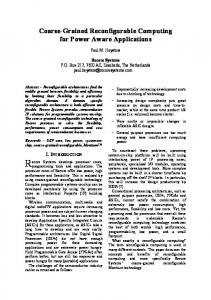
Figure 2. Relative error E, given by eq. (57), between between the reconstructed density PS and the full PS from the N-body simulations, as a function of the parameter α and for two different redshift.
method remains at the ∼ 1 − 1.5%. The value of α (z) decreases from the perturbative value, α = 2, signaling that the contribution from the UV becomes less important than the 1-loop SPT.+ We also see that the range of α where the reconstruction works becomes narrower at low redshifts. This is an indication that the impact of the source becomes more relevant at these redshifts, so that a mistake in its characterization (namely, in its evolution encoded by α) results in a greater penalty in the reconstruction. 6. Cosmology dependence In the previous section we have seen that the nonlinear PS from N-body simulations can be reproduced at the percent level up to k ∼ 0.4 h Mpc−1 by using the expression at the RHS of eq. (51). The first two terms in that expression are 1-loop quantities, which can be computed very rapidly for any cosmology. On the other hand, the third h,N−body quantity, namely, ∆P¯11 , is obtained from an N-body simulation, which typically requires much longer computing times. A fully legitimate question is of course why the use of the RHS of eq. (51) should be convenient with respect to directly using its LHS, that is, taking the nonlinear h,N−body PS entirely from simulations. One first answer is that since the ∆P¯11 term mostly matters at small scales, it typically requires smaller simulation volumes, and +
This may be understood as an effect of the decoupling of short scales consequent to their virialization [11], which would induce an effective UV cutoff, decreasing with z, in the loop integrals. A more thorough analysis is needed to verify this interpretation.
A coarse grained perturbation theory for the Large Scale Structure z 0 0.25 0.5 1 1.5 z 0 0.25 0.5 1 1.5
A− s : αrec. 1.83+0.06 −0.06 1.88+0.09 −0.08 1.96+0.11 −0.10 2.04+0.14 −0.12 2.09+0.17 −0.14 : αrec. n+ s +0.06 1.59−0.05 1.65+0.08 −0.08 1.73+0.11 −0.10 1.85+0.15 −0.13 1.95+0.18 −0.15
err. 0.9% 0.9% 0.9% 0.7% 0.6% err. 1.3% 1.5% 1.5% 1.3% 1.0%
αscal. 1.86 1.88 1.95 2.00 αscal. 1.70 1.75 1.73 1.79
A+ s : αrec. 1.61+0.05 −0.05 1.66+0.07 −0.07 1.74+0.10 −0.09 1.85+0.13 −0.11 1.95+0.15 −0.13 Ω− m : αrec. 1.92+0.07 −0.07 2.01+0.15 −0.13 2.10+0.28 −0.22 2.23+0.45 −0.31 2.30+0.51 −0.34
err. 1.2% 1.4% 1.4% 1.2% 0.9% err. 1.0% 1.4% 2.0% 1.8% 1.3%
αscal. 1.70 1.74 1.75 1.80 αscal. 1.90 1.91 1.94 2.01
n− s : αrec. 1.86+0.05 −0.05 1.91+0.07 −0.06 1.98+0.10 −0.09 2.07+0.12 −0.11 2.11+0.14 −0.12 Ω+ m : αrec. 1.60+0.08 −0.07 1.65+0.07 −0.07 1.71+0.08 −0.07 1.81+0.08 −0.08 1.88+0.10 −0.09
16 err. 0.8% 0.7% 0.8% 0.7% 0.5% err. 1.7% 1.3% 1.1% 0.7% 0.6%
αscal. 1.87 1.89 1.93 1.99 αscal. 1.72 1.74 1.76 1.79
± ± Table 3. Parameter α obtained from the best fit in eq. (56) for the A± s , ns , and Ωm cosmologies listed in Table (1), and for several redshifts.
less realizations, than a simulation aiming at reproducing the PS at all scales, including the linear or almost linear ones. In our approach, these scales are treated by PT, while the N-body simulations are employed only for the scales in which they are really needed. An even more attractive possibility would be to be able to parameterize the h,N−body dependence of the ∆P¯11 term on the cosmology and on time in a simple way, so that, once it is measured carefully from a given N-body simulation, it can be easily “translated” to another cosmology and/or redshift. If this would be possible, then it would open the way to a method for the systematic scanning of different models in the nonlinear regime. In this and in the next section we show that this is indeed possible. First of all, we repeat the procedure described in the previous section to obtain the exponent in eq. (53) from the fit of eq. (51) to the output of the Coyote emulator, for all the other cosmologies in our suite, see Table 1. The results are given in Table 3, from which we see that percent accuracies can be obtained also for these cosmologies. Next, we discuss the truly non-perturbative contribution to eq. (51), namely, of h,N−body ¯ ∆P11 . From eq. (55) we see that its scale dependence is entirely encoded in the correlator hh2 (k, η) ϕ¯1 (k0 , η)i0 . In Figure 3 we plot the ratios between these correlators computed in the cosmologies of Table 1 and the one computed in the reference cosmology, for two different redshifts. As we see, all the ratios are approximately constant in the − whole range of relevant scales. The curves for the cosmologies Ω+ m and Ωm exhibit some wiggles in the BAO range of scales, which are expected from the fact that, already at the linear level, the BAO peaks are shifted in these cosmologies with respect to the REF one. On the other hand, the other four cosmologies in Table 1 have the same growth function and H(z) as the REF cosmology, and therefore the same peak positions. In principle, − the residual wiggles in the Ω+ m and Ωm curves can be eliminated, or reduced, by using the linear information about the peak shifts, however, in this paper we will not do so since the residual scale dependence does not worsen the accuracy of the reconstruction
A coarse grained perturbation theory for the Large Scale Structure
1.6
17
1.6
A+
A+
1.4 < h2 1 >’i / < h2 1 >’REF
< h2 1 >’i / < h2 1 >’REF
1.4 n+
1.2 +
1
REF -
0.8
n-
n+ +
1.2
REF
1
-
0.8 n
A-
0.6 0.1
0.15
0.2
0.25
0.3
k [h Mpc-1]
0.35
0.4
0.6 0.45
0.5
A-
0.1
0.15
0.2
0.25
0.3
k [h Mpc-1]
(z=0)
0
-
0.35
0.4
0.45
(z=1.5)
0
Figure 3. Ratios hh2 (k, η) ϕ¯1 (k0 , η)ii / hh2 (k, η) ϕ¯1 (k0 , η)iREF for the cosmologies in Table 1 and for two different redshifts. The label on each line indicates the cosmology at the numerator.
above the percent level (see below). hϕ ¯ h i0 Due to the approximate scale invariance of the hϕ¯1 h12 i20 i , we can in principle employ REF the hϕ¯1 h2 i0REF correlator for the reconstruction of the PS of any other cosmology up to an overall (i.e. k−independent) rescaling factor, without the need of computing the source from an N-body simulation for that cosmology. We now show that this rescaling factor, and actually an even better k−independence, can be obtained if we also employ information encoded both in SPT and in the time dependence of eq. (53). More specifically, we will consider, for each cosmology, the ratio hh2 (k, η) ϕ¯1 (k0 , η)i0i Ri (k, η) ≡ . (59) ∆P¯ h,1−loop (k, η) ss,11,i
The time dependence of the numerator is given by eq. (53), while that of the denominator is simply ∝ Di2 , therefore �α (η)−2 � Di (η) i , (60) Ri (k, η) ∼ Ri (k, η∗ ) Di (η∗ ) where η∗ corresponds to a redshift at which αi has converged to its SPT value, αi (η∗ ) ' αSP T = 2. If this is the case, Ri (k, η) = Ri (k, η∗ ) for all η < η∗ . At very early time, we expect that the nonperturbative effects should be negligible, and therefore Ri (k, η) should be nearly cosmology- and momentum- independent. Therefore, we expect the ratio � �αREF (η)−2 DREF (η) DREF (η∗ ) Ri (k, η∗ ) b i (k, η) ≡ Ri (k, η) R , (61) � �αi (η)−2 ∼ RREF (k, η) RREF (k, η∗ ) Di (η) Di (η∗ )
b i for the same to be approximately equal to one. In Figure 4 we plot the ratios R cosmologies and redshifts considered in Figure 3. We note that the rescaled ratios are
0.5
A coarse grained perturbation theory for the Large Scale Structure
18
much closer to one than those shown in Figure 3.
1.2
1.2
REF AA+n n+-
1.15 1.1
REF AA+n n+-
1.15 1.1
+
+
i
1.05
1
ˆ R
ˆ R
i
1.05
1
0.95
0.95
0.9
0.9
0.85
0.85
0.8
0.1
0.15
0.2
0.25
0.3
0.35
-1
(z=0)
k [h Mpc ]
0.4
0.45
0.8
0.5
0.1
0.15
0.2
0.25
0.3 -1
k [h Mpc ]
0.35
0.4
0.45
(z=1.5)
ˆ i in eq. (61) for two different redshifts. Notice the range in the Figure 4. Ratios R ˆ i differ y−axis is significantly smaller than the one in Figure 3 and that the ratios R from one by at most a few percent.
7. PS reconstruction for a new cosmology without running a new N-body In this section we will use the results of the previous one to put our method at work, namely to use it to predict a nonlinear PS for a given cosmology without actually running a N-body simulation for that cosmology. Using eq. (61) to relate the hhϕi ¯ correlators of different cosmologies, and (55), we obtain the predicted PS for the i-cosmology given the nonlinear correlator measured for the REF cosmology, hhϕi ¯ REF as 4 0 h,N−body ∆P¯11,i (k, η) ' − hh2 (k, η) ϕ¯1 (k0 , η)ii , αi (η) [5 + 2αi (η)] � �αi (η)−2 Di (η) Di (η∗ ) 4 h,1−loop '− RREF (k, η) ∆P¯ss,11,i (k, η) , � � αi (η) [5 + 2αi (η)] DREF (η) αREF (η)−2 DREF (η∗ )
(62) which is then inserted in (51) to obtain the nonlinear PS for the i-cosmology: 1−loop P¯11,i (k, η) ' P¯ss,11,i ( ) � �α (η)−2 DREF (η∗ ) REF hh2 (k, η) ϕ¯1 (k0 , η)i0REF h,1−loop − 1 + Ci (η) ∆P¯ss,11,i (k, η) , h,1−loop ¯ DREF (η) ∆Pss,11,REF (k, η)
(63) where we have defined 4 Ci (η) ≡ αi (η) [5 + 2αi (η)]
�
Di (η) Di (η∗ )
�αi (η)−2 .
(64)
0.5
A coarse grained perturbation theory for the Large Scale Structure z 0 0.25 0.5 1 1.5 z 0 0.25 0.5 1 1.5
A− s : αCGPT 2.18+0.59 −0.50 2.00+0.63 −0.26 2.02+0.32 −0.23 2.07+0.20 −0.16 2.11+0.16 −0.14 : αCGPT n+ s +0.29 1.53−0.17 1.62+0.26 −0.18 1.71+0.26 −0.19 1.86+0.20 −0.16 1.96+0.18 −0.15
err. 0.9% 0.9% 0.9% 0.7% 0.6% err. 1.3% 1.5% 1.6% 1.2% 0.9%
A+ s : αCGPT 1.47+0.22 −0.14 1.56+0.20 −0.15 1.67+0.22 −0.17 1.83+0.18 −0.15 1.94+0.15 −0.13 Ω− m : αCGPT 2.25+0.69 −0.58 2.3+2.1 −0.5 2.3+4.8 −0.5 2.27+0.74 −0.43 2.29+0.51 −0.34
err. 1.2% 1.4% 1.5% 1.2% 0.9% err. 1.1% 1.5% 2.0% 1.8% 1.3%
n− s : αCGPT 2.18+0.56 −0.49 1.99+0.41 −0.22 2.01+0.28 −0.20 2.07+0.17 −0.15 2.12+0.13 −0.12 Ω+ m : αCGPT 1.57+1.59 −0.23 1.60+0.21 −0.15 1.68+0.16 −0.13 1.81+0.11 −0.10 1.90+0.09 −0.08
19 err. 0.8% 0.8% 0.9% 0.7% 0.5% err. 1.6% 1.2% 1.0% 0.7% 0.5%
Table 4. Parameter α obtained from the Coarse Grained Perturbation Theory ± ± reconstruction of the cosmologies A± s , ns , Ωm . eq. (63) is used, which only requires the source for the REF cosmology from N-body (rather than the sources of all the cosmologies).
The RHS of eq. (63) constitutes our reconstruction for the density PS of any given cosmology (recall that the index i labels any arbitrary cosmology). Apart from the coefficient Ci (η), this RHS can be evaluated without the need to obtain the source for that cosmology from an N-body simulation. When trying to see whether a set of density data is compatible with a given cosmology, we can insert (64) into (63), and leave αi (η) as a free coefficient, which should be fitted together with the data. The error interval for α in Table (4) (see below) shows that α does not need to be determined with a percent accuracy for the final PS to be percent accurate, but that in most cases even a 10% − 20% accuracy is enough. Alternatively, one can evaluate and table the coefficients Ci (η) for a grid of cosmologies, and then interpolate. We now apply this reconstruction procedure to the last 6 cosmologies of Table 1, pretending that we have not evaluated the sources hh2 ϕ¯1 ii for them. In this way we can infer the value of αi (η) that minimizes the difference between the LHS and RHS of (63). We define this quantity as αCGPT (η), and we define the error in this procedure, err.CGPT , and the range ±∆αCGPT (η), precisely as we did for the analogous quantities in Table 3. We show these results in Table 4. The comparison between the “rec.” quantities of Table 3 and the “CGPT” ones of Table 4 quantify how the procedure discussed in this section allows to reconstruct the sources in the i−cosmology without running the corresponding N-body simulation. The interval for αCGPT shown in the table gives a measure of the mistake that can be tolerated in the determination of αCGPT from fitting the data. We recall that this interval indicates the values of α that, once inserted in (64) and then in (63) result in an error that is at most twice the one obtained for the best fit value αCGPT .
A coarse grained perturbation theory for the Large Scale Structure
20
Cosmology REF A− A+ n− n− Ω− Ω+ s s s s m m βi 0.49 0.39 0.51 0.38 0.54 0.58 0.42 Table 5. Slopes of the best linear fit to α(η) for the different cosmologies, defined in eq. (65).
The big “error bars” in Tab. 4 indicate that eq. (63) is only mildly dependent on the parameter αi (η). As we already mentioned, this implies that the parameter αi does not need to be determined with percent accuracy to obtain a percent accurate PS. For all cosmologies and for all redshifts the values in Table 4 (for which, we recall, hh2 ϕ¯1 ii has not been computed) are compatible with those obtained for the REF cosmology in Table 2 (for which hh2 ϕ¯1 ii has been computed). This indicates that the bulk of the h,1−loop cosmology dependence is captured by the perturbative term ∆P¯ss,11,i (k, η) in eq. (63), and in particular it confirms that percent accuracy can be obtained without the need of running N -body simulations for each cosmology. 8. Time dependence of the α parameter. We now discuss the time-dependence of the αi (η) for the different cosmologies, as reported in Table 2 for the REF cosmology and in Table 3 for the other ones. In Figure 5 we plot the time-dependent values of Tables 2 and 3 (red points with error bars) and we notice that the central values are very well fit by a linear dependence in η (red lines). The best fit slopes for each cosmology, defined as dαrec.,i , (65) dη where αrec.,i is the best linear fit to the i-th cosmology, are given in Table 5. To gauge the sensitivity of our reconstruction procedure on the time-dependence of the αi ’s we also plot, for each cosmology, the two dashed lines, corresponding to βi ≡ −
αimin (η) = αi (η0 ) − (η − η0 ) β min ,
αimax (η) = αi (η0 ) − (η − η0 ) β max , (66)
where β min = 0.38 (β max = 0.58) is the smallest (largest) β in Table 5. As one can notice, taking any value of the slope between these two extrema gives values of αi inside the error bars at any redshift. This result is very encouraging, as it shows that once αi is fixed at z = 0 in a given cosmology, either by direct fitting or by the procedure described in the previous section, its values at higher redshifts can be reproduced accurately enough by assuming a linear dependence with the slope provided by, e.g. the REF cosmology. This provides further confirmation of the robustness of our Ansatz for the time dependence of the correlators, eq. (53) and, more practically, it shows that we do not need extra parameters to characterize the cosmological dependence of the time evolution.
A coarse grained perturbation theory for the Large Scale Structure
21
2.8
REF
2.6 2.4 2.2 2 1.8 1.6 -0.8
-0.7
-0.6
-0.5
2.8
-0.4
-0.3 - 0
-0.2
0
0.1
2.8 -
2.6
A+
2.6
A
2.4
2.4
2.2
2.2
2
2
1.8
1.8
1.6 -0.8
-0.1
1.6 -0.7
-0.6
-0.5
-0.4
-0.3
-0.2
-0.1
0
0.1
-0.8
-0.7
-0.6
-0.5
-0.4
- 0
2.8
n
-
2.6
2.4
2.4
2.2
2.2
2
2
1.8
1.8
1.6
-0.1
n
0
0.1
0
0.1
0
0.1
+
1.6 -0.7
-0.6
-0.5
-0.4
-0.3
-0.2
-0.1
0
0.1
-0.8
-0.7
-0.6
-0.5
-0.4
- 0
2.8
-0.3 - 0
-0.2
-0.1
2.8 -
2.6
+
2.6
2.4
2.4
2.2
2.2
2
2
1.8
1.8
1.6 -0.8
-0.2
2.8
2.6
-0.8
-0.3 - 0
1.6 -0.7
-0.6
-0.5
-0.4
-0.3 - 0
-0.2
-0.1
0
0.1
-0.8
-0.7
-0.6
-0.5
-0.4
-0.3 - 0
-0.2
-0.1
Figure 5. The time-dependent αi ’s for the different cosmologies of our simulation suite. For each cosmology, the solid orange line indicates the best linear fit to the η dependence, while the black dashed lines are obtained from the largest (β = 0.58) and the smallest (β = 0.38) slope in Table 5. .
A coarse grained perturbation theory for the Large Scale Structure
22
9. Comparison with EFT approach In this section we discuss the relationship between our approach and the Effective Field Theory of Large Scale Structure (EFToLSS) approach of [11, 12, 15]. A good starting point to do so is eq. (39) hϕ¯a (k, η)ϕ¯b (k0 , η 0 )i = hϕ¯ss,a (k, η)ϕ¯ss,b (k0 , η 0 )i (1)
¯ss,b (k0 , η 0 )i + hϕ¯ss,a (k, η)ϕ¯σ,b (k0 , η 0 )i + O(hσ 2 i) , + hϕ¯(1) σ,a (k, η)ϕ
(67)
in which, we recall, the first term at the RHS is the fully nonlinear PS in the single stream approximation, while the other two give the effect of small scale velocity dispersion at linear order in σ, Z η (1) 0 0 hϕ¯σ,a (k, η)ϕ¯ss,b (k , η )i = − ds gac (η − s) hδhc (k, s) ϕ¯ss,b (k0 , η 0 )i . (68) ηin
Considering the density PS and using a notation analogous to that of Section 3 we can write � 1−loop n≥2−loop lin δh P¯11 (k, η) = P¯11 (k, η)+ P¯ss,11 (k, η)+ P¯ss,11 (k, η)+∆P¯11 (k, η)+O σ 2 , (69) where we have split the single stream contribution in its linear plus 1-loop n≥2−loop approximation, and all higher order terms, P¯ss,11 (k, η). The L-dependence of the 2 ˜ [kL] one, and therefore we have omitted it, or, various terms is just the trivial W equivalently, one can imagine taking the limit L → 0.
z=0 z=0.25 z=0.5 z=1 z=1.5
2
cs2 (h Mpc-1 / kNL)2
2
1.5
1
0.5
0 0.05
0.1
0.15
0.2
0.25
0.3
0.35
0.4
0.45
0.5
k [h Mpc-1]
Figure 6. Ratio in eq. (71) at 5 different redshift in the REF cosmology.
A coarse grained perturbation theory for the Large Scale Structure
23
The expression above, which is exact up to O(σ 2 ) corrections, should be compared with the lowest order (1-loop) EFToLSS approximation [12, 15], which, in our notation, ˜ 2 [kL] factor from both sides) would read (see eq. (58) of [15]), (and removing the W 1−loop lin P11 (k, η) ' P11 (k, η) + Pss,11 (k, η) − 2(2π) c2s(1)
k 2 lin P (k, η) , 2 kN L
(70)
where we recall that P lin is the linear PS, and where the k-independent parameter c2s(1) can be interpreted as an effective speed of sound, to be determined by fitting the PS with N-body simulations. Higher orders in the EFToLSS include higher loops and 4 higher powers of k/kN L . In [15], contributions up to 2-loop orders and O(k 4 /kN L ) have been included, however we will limit our discussion to the comparison with the 1-loop EFToLSS of eq. (70), for which the derivation is straightforward. Comparing (70) to (69) we immediately understand the physical effects contained in the speed of sound term at this order. Namely, c2s(1) incorporates all the nonlinearities of the pressureless ideal fluid equations beyond 1-loop, plus the effect of the small scale velocity dispersion. In Figure 6 we plot the quantity 1−loop Pss,11 (k, η) − P11 (k, η) , 2 k 2 P l (k, η)
(71) 2πc2
which, according to eq. (70), should correspond to the k-independent quantity k2s(1) . In NL ref. [15] the speed of sound was determined by fitting eq. (70) to the nonlinear PS in the � � −1 2 k ∼ 0.15 − 0.25 h Mpc−1 range, obtaining in this way 2πc2s(1) h Mpc = 1.62 ± 0.03 kN L for z = 0. As we see, the central value is consistent with the z = 0 curve of the REF cosmology shown in Figure 6. However the residual BAO fluctuations – coming from the difference between the 1-loop PS and the nonlinear PS– are quite strong, and the difference between the lines in Figure 6 and a constant gives a measure of the error made in the measurement of c2s(1) by ordering the corrections by simple power counting in k/kN L when the PS is not a simple power-law, but has scale dependent features such as BAO’s. This error propagates, in a reduced manner proportional to the size of the correction, to the final reconstruction of the PS. In [18] these residual fluctuations were reduced by resumming the effect of particle displacements at all orders in SPT. Moreover, the sound speed defined according to eq. (70) exhibits a significant cosmology dependence. We show this in Figure 7, where we plot the ratio (71) at redshift z = 0 for the cosmologies in Table 1. If we adopt the prescription of [15] that consists in determining the sound speed from the average of this result in the k ∼ 0.15 − 0.25 h Mpc−1 range we obtain the numerical values reported in Table 6. In the approach followed in this paper, on the other hand, we do not send the cutoff L → 0, but we keep it fixed at a scale such that the 1-loop expression holds for the < 1/L and we use the N-body simulations to replace the 1-loop contributions for scales k ∼ > 1/L with the fully non-perturbative ones. The scale dependence of the correction to k∼ the 1-loop result is therefore taken into account more carefully. In the previous sections
A coarse grained perturbation theory for the Large Scale Structure
3
REF AA+n n+-
2.5
+
2 1.5
2
cs2 (h Mpc-1 / kNL)2
3.5
24
1 0.5 0.05
0.1
0.15
0.2
0.25 -1
k [h Mpc ]
0.3
0.35
0.4
0.45
0.5
(z=0)
Figure 7. Dependence of the sound speed on the cosmologies in Table 1. The curves show the ratio in eq. (71) for these cosmologies at z = 0.
REF A− s
Cosmology “Average” 2πc2s(1)
�
� −1 2
h Mpc kN L
1.64
A+ s
n− s
n+ s
Ω− s
Ω+ s
1.21 2.34 1.39 2.02 1.39 1.78
Table 6. Cosmology dependence of the rescaled sound speed, defined as in [15] from the average of eq. (71) in the k ∼ 0.15 − 0.25 h Mpc−1 range, at z = 0.
we have discussed how, once this has been measured for a given redshift and a given cosmology, it can be used for reconstructing the full PS at different redshifts and for different cosmologies. Our approach suggests a definition of effective sound speed different from (71), namely, Rη 2 ds g12 (η − s)hδh2 (k, s)ϕ¯1 (k0 , η)i0 k η 2π¯ c2s 2 ≡ in kN L hϕ¯1 (k, s)ϕ¯1 (k0 , η)i0 ! h,1−loop h,N−body 1 ∆P¯11 (k, η) ∆P¯ss,11 (k, η) =− − + O(2 − loop) . (72) N−body 1−loop 2 P¯11 (k, η) P¯ss,11 (k, η) The first line in the above definition relates directly the effective speed of sound to the non-perfect fluid effects, that is, it exactly vanishes in the single stream approximation, and, moreover, it is exactly independent on the cutoff L. This is not true any more by truncating the PT expansion of hss,2 at a finite order, as we do at the second line. Still, even at this order, the scale dependence is greatly reduced with respect to that
A coarse grained perturbation theory for the Large Scale Structure
25
of the expression in eq. (71), since taking ratios N-body/N-body and PT/PT cancels the residual BAO’s much more efficiently. This is explicitly shown in Figure 8. We see however a residual scale dependence at the highest momenta shown, which is to be interpreted as the effect of neglecting 2−loop contributions ∝ k 4 in this computation.
z=0 z=0.25 z=0.5 z=1 z=1.5
2
cs2 (h Mpc-1 / kNL)2
2
1.5
1
0.5
0 0.1
0.15
0.2
0.25
0.3
0.35
0.4
0.45
0.5
k [h Mpc-1]
Figure 8. Sound speed defined according to our eq. (72) at 5 different redshift in the REF cosmology. We notice that the k−depence due to the BAO oscillations is significantly less pronounced than the one obtained from the prescription (71), and shown in Figure 6.
10. Conclusions In this paper we have shown that the lowest order approximation in the CGPT approach, namely, a 1-loop computation for the IR modes and the measurement of only one crosscorrelator between the UV source term and the density field, is able to reproduce the < 0.4 h Mpc−1 . The cross-correlator appears in nonlinear PS at the percent level up to k ∼ a time integral, eq. (52), which would require measuring it by cross-correlating different N-body snapshots. Instead, we approximate the time dependence with the SPT-inspired Ansatz (53), which allows an analytical evaluation of the integral. This introduces a free parameter, α(η), which can be measured either by fitting the reconstructed PS to the nonlinear one, or by direct measurement of the scaling with time of the cross-correlator in the IR regime. The results from the two approaches give compatible results, which corroborates the Ansatz (53). Once the cross-correlator and α(η) have been measured in a given cosmology, they
A coarse grained perturbation theory for the Large Scale Structure
26
can be used for a different one by using eq. (63). Therefore we do not need to run an N-body simulation for each cosmology. Most of the cosmology dependence is encoded in h,1−loop the 1-loop SPT quantity ∆P¯ss,11,i (k, η). The residual dependence in the Ci (η) factor is a very shallow one, as we read from the large error bars in Table 4 , and, at least for the cosmologies we considered, it can be neglected by setting Ci (η) = CREF (η). The same holds for the time dependence (the slope) of the αi functions, as we discussed in Section 8. In any case, a very robust feature of the UV contribution emerges from this investigation, namely the scale-independent ratios of Figure 3 between the source-density cross-correlators computed for different cosmologies. This shows that a single scaleindependent parameter is enough to describe the cosmology change. In our approach, we have shown that this parameter can be mostly reproduced by a proper SPT computation, Figure 4, but one could also take the agnostic view of simply marginalizing over it in a parameter estimation procedure. Due to the scale independence, this will probably have small impact on extracting cosmological parameters from BAO observations. It will be very important to extend the analysis of this paper to an enlarged set of cosmological models: massive neutrinos, modifications of General Relativity, clustering Dark Energy, and so on, to investigate to what extent the scale independence of Figure 3 holds also for these less standard scenarios. An analytic understanding of the behavior of these UV sources, e.g. in the halo model, would be precious in order to better understand the physical reason for the scale independent ratios (which is however already in agreement with SPT) and to predict the time-dependence of the αi (η) exponents. On a more theoretical side, a next order computation (2-loop, O(σ 2 )) would probably not improve too much the results in the BAO region, but it would provide useful information on issues such as the smallest scales which can be described by such method, and would mitigate further the cutoff dependence of the results. Acknowledgments We thank G. Mangano and L. Hui for discussions. M. Peloso would like to thank the University of Padova, Dipartimento di Fisica e Astronomia, and the INFN, Sezione di Padova, for their friendly hospitality and for partial support during the earlier stages of this work. M. Pietroni would like to thank the Institute for Theoretical Physics of the University of Heidelberg for their friendly hospitality and for partial support during the later stages of this work. A. Manzotti acknowledges partial support from the Kavli Institute for Cosmological Physics at the University of Chicago through grants NSF PHY-1125897 and an endowment from the Kavli Foundation and its founder Fred Kavli. M. Peloso acknowledges partial support from the DOE grant de-sc0011842 at the University of Minnesota. M. Pietroni acknowledges partial support from the European Union FP7 ITN INVISIBLES (Marie Curie Actions, PITN- GA-2011- 289442). M. Viel and F. Villaescusa-Navarro are supported by the ERC StG ”cosmoIGM” and by INFN IS PD51 ”INDARK” grants.
A coarse grained perturbation theory for the Large Scale Structure
27
Appendix A. Check of the L-factorization in the 1-loop density PS in single stream approximation The filtering operation commutes with the expansion in the microscopic velocity dispersions. A consequence of this are the identities written in eq. (37) and in the following line of the main text. Each of these identities is actually valid order by order in ϕlin . Therefore, the simplest nontrivial identity gives rise to the expression 1−loop ˜ 2 (kL) P11 (k, η) . hϕ¯ss,1 (k, η) ϕ¯ss,1 (k0 , η)i01−loop = W
(A.1)
In this appendix we explicitly verify this relation, as a check on our expansion scheme. Our starting point is the system (23) for the fields in single stream approximation. Is is convenient to define ϕ¯ss,a (k, η) = ϕ¯(h=0) (k, η) + ϕ¯(h) a a (k, η) ,
(A.2)
where ϕ¯(h) a (k, η)
Z
η
≡−
ds gab (η − s)hss,b (k, s) .
(A.3)
ηin
To obtain the 1-loop PS, we need to expand ∗ = ϕ¯(h=0,1) + ϕ¯(h=0,2) + ϕ¯(h=0,3) +O ϕ¯(h=0) a a a a � � �4 ϕ¯(h) = ϕ¯(h,2) + ϕ¯(h,3) + O ϕlin , a a a
�
ϕlin
�4 �
, (A.4)
where we keep into account that hss is at least quadratic in the linear fields. Indeed, the (h) terms in the expansion in ϕ¯a can be immediately obtained by expanding the source hss in (A.3), and, expanding (31) and (32), we see that � i 2 3 J1,ss = hδss ∂i φss i − δ¯ss h∂i φss i − δ¯ss hδ∂i φss i + δ¯ss h∂i φss i + O δss φss , � i i k i k i k i k i k Jσ,ss = ∂k hvss vss i − ∂k v¯ss v¯ss + ∂k hδss vss vss i − δ¯ss ∂k hvss vss i − v¯ss v¯ss ∂k δ¯ss � 2 2 + O δss vss . (A.5) (h=0)
To obtain ϕ¯a we instead insert (A.2) and (A.3) into the system (23). We obtain (h=0) that the field ϕ¯a satisfies (h=0)
(δab ∂η + Ωab )ϕ¯b
(h=0)
(k, η) = Ik,q1 ,q2 eη γabc (q1 , q2 )ϕ¯b
(q1 , η)ϕ¯(h=0) (q2 , η) c
(h=0)
+ 2 Ik,q1 ,q2 eη γabc (q1 , q2 )ϕ¯b
(q1 , η)ϕ¯(h) c (q2 , η) � �� (h=0) ab lin 4 (q2 , η) + O ϕ . − Ik,q1 ,q2 Dω (q1 , q2 )ϕ¯b (A.6)
The last explicit term � in �this � expression originates from the last term in (23), 2 with only the leading O ϕlin contribution retained in the expression (28) for the ∗ We stress that the order in each term refers to the number of linear fields contained in it. Contrary, for example to eq. (35), these expressions are not series expansions in the microscopic σ. All this appendix assumes single stream approximation, σ = 0).
A coarse grained perturbation theory for the Large Scale Structure
28
vorticity: ! � � 1 0 q2 · q1 q1 · p2 q2 · p2 2η ab − e Iq1 ,p1 ,p2 Dω (q1 , q2 ) = q 2 +2 q ·q 0 2 q2 1 2 q12 p22 p22 2 ab h i � �� ˜ (q1 L) − W ˜ (p1 L) W ˜ (p2 L) ϕlin (p1 ) ϕlin (p2 ) + O ϕlin 3 . × W (A.7) � � 4 or We also note that the hωa term in (23) contributes to (A.6) only at O ϕlin higher, and the vorticity is at least quadratic in the linear fields. Therefore, this term is irrelevant for the present computation. We now proceed by explicitly computing the terms in (A.4), and then the 1loop power spectrum. We evaluate the 1-loop mode-mode coupling contribution, (22) (13) also identified as PP T in the standard PT terminology, separately from the PP T contribution, and we verify that they separately satisfy the identity (A.1). We then conclude this appendix by collecting the results that give the 1-loop PS for the density fields entering in eq. (46). �
(22)
Appendix A.1. PP T contribution We now compute (2)
00 0h hh hϕ¯(2) ¯b (k0 , η)i = Cab + Cab + Cab , a (k, η)ϕ
(A.8)
where (h=0,2)
00 Cab ≡ hϕ¯(h=0,2) (k, η)ϕ¯b a
(h,2)
0h Cab ≡ hϕ¯(h=0,2) (k, η)ϕ¯b a
(h,2)
hh Cab ≡ hϕ¯(h,2) (k, η)ϕ¯b a
(k0 , η)i , (h=0,2)
(k0 , η)i + hϕ¯(h,2) (k, η)ϕ¯b a
(k0 , η)i ,
(k0 , η)i .
(A.9)
Only the first line of (A.6) and the leading expressions in (A.5) contribute to the second order fields. We obtain Z η (h=0,2) ϕ¯a (k, η) = ds gac (η − s)es Ik,q1 ,q2 ˜ [q1 L]W ˜ [q2 L] ϕlin (q1 )ϕlin (q2 ) , × γcde (k, q1 , q2 )ud ue W
(A.10)
and ϕ¯(h,2) (k, η) a
Z =
η
ds gac (η − s)es Ik,q1 ,q2
h ˜ [kL] − W ˜ [q1 L]W ˜ [q2 L]) ϕlin (q1 )ϕlin (q2(A.11) (k, q1 , q2 )ud ue (W ), × γcde h where we have defined a new “vertex” function γcde , whose only non vanishing elements are, � � 3 Ωm k · q1 k · q2 h + , γ211 (k, q1 , q2 ) = 4 f2 q12 q22 k · q1 k · q2 h γ222 (k, q1 , q2 ) = . (A.12) q12 q22
A coarse grained perturbation theory for the Large Scale Structure
29
We then obtain (00,0h,hh)
Cab
= 2 (2π)3 δD (k + k0 )Ik,q,p P l (q) P l (p) Z η Z η 0 (00,0h,hh) s ds0 gbd (η − s0 )es ue uf ug uh Acef dgh , ds gac (η − s)e ×
(A.13)
where P l is the power spectrum of the linear fields, and where (00) ˜ [qL]2 W ˜ [pL]2 , Acef dgh = γcef (k, p, q)γdgh (k, p, q)W � � (0h) h h Acef dgh = γcef (k, p, q)γdgh (k, p, q) + γcef (k, p, q)γdgh (k, p, q) � � ˜ [kL] − W ˜ [pL]W ˜ [qL] W ˜ [pL]W ˜ [qL] , × W � �2 (hh) h h ˜ [kL] − W ˜ [pL]W ˜ [qL] . Acef dgh = γcef (k, p, q)γdgh (k, p, q) W (A.14)
We now add the three contributions as in (A.8), and set a = b = 1 for the mode coupling part of the PS of the density field. By using the explicit expressions for the vertices we obtain (2)
(2)
(22)
˜ [kL]2 P (k, η) . hϕ¯1 (k, η)ϕ¯1 (k0 , η)i = (2π)3 δD (k + k0 )W PT
(A.15)
showing that the mode coupling contribution to the density PS factors out the filter function, in agreement with (A.1). (13)
Appendix A.2. PP T contribution These contribution to the PS is obtained by correlating ˜ [kL] φl (k) ua , ϕ¯(h=0,1) (k, η) = W a
(A.16)
with the third order terms in the expansion (A.4). (h=0,3) Let us first discuss the terms with ϕ¯a in the correlator. One contribution to (h=0,3) ϕ¯a is obtained from a diagram with two vertices coming both from the first line in eq. (A.6) (in practice, we use eq. (A.10) alternatively for the two fields at the first term at RHS of eq. (A.6)). This gives (h=0,1)
hϕ¯(h=0,3) (k, η)ϕ¯ (k0 , η)iγγ + (a ↔ b) = 4 (2π)3 δD (k + k0 ) a Z η Z bs 0 ds ds0 es+s gac (η − s)P l (k)Ik,q,p P l (q)ue ug uh ub × ˜ [kL]2 + (a ↔ b) . ˜ [qL]2 W γcde (k, p, q)gdf (s − s0 )γf gh (p, q, k)W Another contribution to of (A.6). This gives
(h=0,3) ϕ¯a
(A.17)
is obtained by using eq. (A.11) in the second line
(h=0,1)
hϕ¯(h=0,3) (k, η)ϕ¯b (k0 , η)iγγ h + (a ↔ b) = 4 (2π)3 δD (k + k0 ) a Z η Z s 0 ds ds0 es+s gac (η − s)P l (k)Ik,q,p P l (q)ue ug uh ub × � � 2 ˜ 2 0 h ˜ ˜ ˜ ˜ γcde (k, p, q)gdf (s − s )γf gh (p, q, k) W [kL]W [qL]W [pL] − W [qL] W [kL] + (a ↔ b) .
(A.18)
A coarse grained perturbation theory for the Large Scale Structure
30
(h=0,3)
The third and final contribution to ϕ¯a comes from the third line of (A.6), the vorticity term, in which we use (A.7). This gives (h=0,1)
hϕ¯(h=0,3) (k, η)ϕ¯b (k0 , η)ih0ω + (a ↔ b) = − (2π)3 δD (k + k0 ) a � � Z η q2 + 2 p · q 2s l l ds e P (k)Ik,q,p P (q) ga1 (η − s) u1 + ga2 (η − s) u2 ub × q2 � � � (q · p)2 q · p k · p k · q � ˜ ˜ [qL]W ˜ [pL] − W ˜ [kL]2 W ˜ [qL]2 1− 2 2 + − W [kL] W pq k 2 p2 k2 + (a ↔ b) . (A.19) (h,3)
The remaining contributions to PP13T have ϕ¯a in the correlator. One of these contribution originates from the PT expansion (namely, eq. (A.10)) of the quadratic terms in the sources (A.5). It gives (h=0,1)
hϕ¯(h,3) (k, η)ϕ¯ (k0 , η)iγ h γ + (a ↔ b) = 4 (2π)3 δD (k + k0 ) a Z η Z sb 0 ds ds0 es+s gac (η − s)P (k)Ik,q,p P (q)ue ug uh ub × � � h 0 2 2 ˜ 2 ˜ ˜ γcde (k, p, q)gdf (s − s )γf gh (p, q, k) W [kL] − W [kL] W [qL] + (a ↔ b) .
(A.20)
(We recall that the quadratic terms already factored a vertex γ h , cf. eq. (A.11), while the vertex γ originates from the PT expansion). Taking into account that the −ϕ¯2 terms in the sources can be expanded also using (A.11), we have also the contribution (h=0,1)
hϕ¯(h,3) (k, η)ϕ¯b (k0 , η)iγ h γ h + (a ↔ b) = −4 (2π)3 δD (k + k0 ) a Z η Z s 0 ds0 es+s gac (η − s)P l (k)Ik,q,p P l (q)ue ug uh ub × ds � � h 0 h 2 ˜ 2 ˜ ˜ ˜ ˜ γcde (k, p, q)gdf (s − s )γf gh (p, q, k) W [kL]W [qL]W [pL] − W [kL] W [qL] + (a ↔ b) .
(A.21)
Then, we have the contribution from the vorticity component of v¯i in Jσi , which gives (h=0,1)
(k0 , η)ih1ω + (a ↔ b) = 2 (2π)3 δD (k + k0 ) hϕ¯(h,3) (k, η)ϕ¯b a " # Z η 2 2 2 k − q (k · q) k · q 1− 2 2 dse2s ga2 (η − s)ub P l (k)Ik,q,p P l (q) 2 q p2 k q � � ˜ [kL]W ˜ [qL]W ˜ [pL] − W ˜ [kL]2 W ˜ [qL]2 + (a ↔ b) . W Finally, the cubic terms in (A.5) give (h=0,1)
hϕ¯(h,3) (k, η)ϕ¯b (k0 , η)ih(3) + (a ↔ b) = (2π)3 δD (k + k0 ) a Z η dse2s ga2 (η − s)ub P l (k)Ik,q,p P l (q) × � � � � 3 Ωm k·q �˜ 2 ˜ 2 ˜ [kL]W ˜ [qL]W ˜ [pL] 1 − W [kL] W [qL] − W 2 f2 q2
(A.22)
A coarse grained perturbation theory for the Large Scale Structure � � (k · q)2 ˜ (k · q)2 (k · q)2 ˜ 2 ˜ [qL]2 − W [kL] + 1 + 2 2 + W [kL]2 W q4 k q q4 � � � q · p k · qk · p ˜ ˜ ˜ + + W [kL]W [qL]W [pL] + (a ↔ b) . q2 k2q2
31
(A.23)
Setting again a = b = 1, the sum of eqs. (A.17) to (A.23) gives (3)
(1)
(13)
˜ [kL]2 P (k, η) , 2hϕ¯1 (k, η)ϕ¯1 (k0 , η)i = (2π)3 δD (k + k0 )W PT
(A.24)
which, together with the result (A.15) completes our check that the only cutoff ˜ [kL]2 , dependence of the 1-loop result for the density density PS is in the overall factor W in agreement with eq. (A.1) of the main text. Appendix A.3. Explicit expressions for the 1-loop PS We now provide the explicit expressions for the 1-loop power spectra used in the main text, cf. eq. (51). We have (22)
(13)
1−loop hϕ¯ss,1 (k, η) ϕ¯ss,1 (k0 , η)i0 ≡ P¯11,ss = P¯11,ss + P¯11,ss .
(A.25)
The mode coupling term evaluated in Appendix A.1 acquires the explicit final expression 1 2η k 3 π e 49 (2π)3 Z 1 Z ∞ � (3r + 7x − 10rx2 )2 � √ l l 2 dx P k 1 + r − 2rx drP (kr) , (1 + r2 − 2rx)2 −1 0
(22) ˜ 2 [k L] P¯11,ss = W
(A.26)
where we recall that P l is the PS of the linear ϕlin fields. The sum of expressions (A.17) to (A.23) gives instead Z ∞ 3 1 (13) 2 l 2η k π ¯ ˜ drP l (kr) P11,ss = W [k L] P (k) 2e 252 0 (2π)3 � � �3 � r + 1 12 3 2 2 4 2 . (A.27) − 158 + 100r − 42r + 3 r − 1 2 + 7r ln r2 r r − 1 We remark that these expressions are the standard 1-loop PT results, times the square of the filter function. We then have Z η 0 − dsg1c (η − s) hhss,c (k, s) ϕ¯ss,1 (k0 , η)i1−loop + (k ↔ k0 ) ηin
=2
D
(h) ϕ¯1
E0 (k, η) ϕ¯ss,1 (k , η) 0
1−loop
h,(22) h,(13) h,1−loop ≡ ∆P¯ss,11 (k, η) = ∆P¯ss,11 (k, η) + ∆P¯ss,11 (k, η)
(A.28)
0h The mode coupling contribution is given by the Cab term in eq. (A.8), and it evaluates to
A coarse grained perturbation theory for the Large Scale Structure
32
Z k 3 e2η ∞ ˜ drW [krL]P l (kr) = 196π 2 0 Z 1 � p � (3r + 7ξ − 10rξ 2 )2 p l 2 ˜ [k 1 − 2rξ + r2 L] dξ P k 1 − 2rξ + r W (1 − 2rξ + r2 )2 −1 � � p 2 ˜ ˜ ˜ W [kL] − W [krL]W [k 1 − 2rξ + r L] . (A.29)
h,(22) ∆P¯ss,11 (k, η)
The other term is obtained by summing the contributions from (A.20) to (A.23), giving 2η 3 l ˜ [kL] Z ∞ 3e k P (k) W h,(13) dr P l (rk) ∆P¯ss,11 (k, η) = − 1512π 2 0 # �" 2 3 2 6 3 (1 − r ) (2 + 7r ) r + 1 ˜ [kL] W 21r4 − 50r2 + 79 − 2 + ln 3 r 2 r r − 1 Z 1 h p i � 28 2 ˜ 2 ˜ [krL] + 2W ˜ [krL] ˜ k 1 + r2 − 2rξL × + 2 − 17r W [kL] W dξ W 3 −1 � 2 3 2 2 (35 + 14ξ ) r − ξ (77 − 56ξ ) r + 5 (13 − 34ξ 2 ) r + 77ξ (r − ξ) .(A.30) 1 + r2 − 2rξ Appendix A.4. Explicit expression of the N-body correlator in the REF cosmology The RHS of eq. (63) is our main result for the density PS of an arbitrary cosmology. For this expression we only need to compute once for all the source in the REF cosmology through an N-body simulation. Specifically, we can rewrite eq. (63) as 1−loop h,1−loop P¯11,i (k, η) ' P¯ss,11,i − {1 + Ci (η) N (k, η)} ∆P¯ss,11,i (k, η) , � �αREF (η)−2 hh2 (k, η) ϕ¯1 (k0 , η)i0REF DREF (η∗ ) N (k, η) ≡ , h,1−loop DREF (η) ∆P¯ss,11,REF (k, η)
(A.31)
where the cosmology-dependent coefficient Ci is given in eq. (64). All the information from the REF cosmology is encoded in the function N (k, η). We give the values of this function at various momenta in our grid and at various redshifts in Tables A1 and A2. These are the values used in Section 7.
A coarse grained perturbation theory for the Large Scale Structure k [h Mpc−1 ] 0.04189 0.05437 0.06709 0.07906 0.09134 0.1037 0.1161 0.1284 0.1406 0.1529 0.1654 0.1777 0.1899 0.2021 0.2144 0.2267 0.239 0.2513 0.2636 0.2758 0.2881 0.3004 0.3126 0.325 0.3373
z=0 -22.769 -14.654 -11.02 -10.784 -10.657 -9.5307 -9.5171 -9.9881 -9.6142 -9.619 -9.8505 -8.7385 -8.5702 -8.6357 -8.5725 -8.7537 -8.3866 -8.4467 -8.3299 -7.8928 -7.8624 -7.7228 -7.4547 -7.2651 -7.169
z = 0.25 -21.978 -14.238 -11.071 -10.618 -10.457 -9.2659 -9.4227 -9.8072 -9.3851 -9.2895 -9.6062 -8.5163 -8.3233 -8.3204 -8.2674 -8.5019 -8.0742 -8.0667 -7.9773 -7.4875 -7.4591 -7.2474 -7.0516 -6.9177 -6.8044
z = 0.5 -20.886 -13.967 -11.007 -10.404 -10.402 -9.1511 -9.2084 -9.579 -9.1766 -9.0581 -9.3549 -8.313 -8.1506 -8.0134 -8.0855 -8.2564 -7.8584 -7.774 -7.6964 -7.1876 -7.1588 -6.9001 -6.7616 -6.6184 -6.5113
z=1 -20.86 -13.922 -10.9 -10.429 -10.299 -9.1649 -9.2901 -9.6157 -9.1628 -8.8711 -9.2146 -8.2408 -8.0763 -7.8816 -7.8846 -8.1066 -7.6715 -7.5224 -7.4345 -6.9159 -6.8676 -6.6069 -6.5887 -6.3522 -6.2678
33 z = 1.5 -20.854 -14.143 -11.228 -10.65 -10.424 -9.3105 -9.4307 -9.6923 -9.1966 -8.9044 -9.1739 -8.2664 -8.0655 -7.8148 -7.8426 -7.9504 -7.6011 -7.4443 -7.2596 -6.7223 -6.7369 -6.4249 -6.4404 -6.1989 -6.1105
Table A1. Table of values for the function N (k, η) defined in eq. (A.31). This table is continued by Table A2.
Appendix B. Choice of the filter scale In this Appendix we discuss the choice of the scale L = 2 h−1 Mpc in the filter function 2 2
˜ (k L) = e− k 2L , W
(B.1)
that we have adopted in our numerical evaluations. As mentioned in Section 4, we use numerical simulations of npart = 5123 particles on a box of Lbox = 512 h−1 Mpc comoving size. The quantities needed for the computation of the sources (15) and (16), namely, particle number density, mass-weighted velocity, acceleration, and velocity dispersion, eq. (9), are measured on a grid of step d = 2 h−1 Mpc. In this way we obtain fields with √ wave numbers up to kmax ' 3π/d ' 2.72 h Mpc−1 in Fourier space, which we consider as our UV fields, that is, the fields without the overbars in eq. (9), (15) and (16). Then,
A coarse grained perturbation theory for the Large Scale Structure k [h Mpc−1 ] 0.3496 0.3618 0.374 0.3863 0.3986 0.4109 0.4232 0.4355 0.4478 0.46 0.4722 0.4845 0.4968 0.5091
z=0 -6.9646 -6.8781 -6.438 -6.3107 -6.218 -5.9557 -5.8415 -5.5195 -5.3941 -5.0666 -5.0114 -4.8651 -4.5482 -4.436
z = 0.25 -6.5528 -6.5329 -6.1324 -5.9708 -5.8443 -5.6486 -5.5234 -5.2324 -5.1071 -4.8823 -4.7449 -4.578 -4.3485 -4.2369
z = 0.5 -6.2584 -6.2598 -5.8862 -5.697 -5.5441 -5.4075 -5.2841 -5.0133 -4.8755 -4.6988 -4.5356 -4.3759 -4.1928 -4.0683
z=1 -6.0055 -5.9708 -5.664 -5.4749 -5.3881 -5.2213 -5.0915 -4.8701 -4.6829 -4.5985 -4.3721 -4.2946 -4.0874 -4.0069
34 z = 1.5 -5.8622 -5.8223 -5.5419 -5.3555 -5.2805 -5.1131 -4.9649 -4.777 -4.6088 -4.4877 -4.2662 -4.2675 -4.0197 -3.9645
Table A2. Continuation of Table A1.
in order to compute the sources, we filter products of the fluctuations of these UV fields √ with the gaussian in (B.1), which damps out wave numbers with k � ksmooth ' 2/L. Since the UV fields are defined only up to kmax , one should have ksmooth � kmax , which √ √ means, L � 2d/( 3π) ' 0.52 h−1 Mpc in our configuration. For this reason, and also to limit the the upper limit of SPT loop integrations (given by ksmooth ) in a reliable range, we did not consider a scale smaller than L = 2 h−1 Mpc for our filter function, corresponding to ksmooth ' 0.71 h Mpc−1 . We stress, however, that the procedure described above takes into account, through the sources, the UV information up to the Nyquist wave number of the simulation, √ 1/3 namely 3 π npart /Lbox h Mpc−1 ' 5.44 h Mpc−1 , and not only up to kmax . Indeed, we could have avoided the intermediate step of defining the UV fields up to kmax , and measure the fields and the sources, filtered at the scale L, starting directly from the particles. We followed the described procedure only for practical purposes, since processing the UV fields once they have been measured from the simulation (e.g., computing the sources and the cross-correlators) can be done on a normal laptop. We performed a comparison between L = 2 h−1 Mpc and L = 4 h−1 Mpc and we obtained a much better reconstruction in the former case. This is illustrated the left panel of Figure B1, which shows the relative error E in the PS reconstruction procedure for the REF cosmology, z = 0 and for the two choices L = 2 h−1 Mpc and L = 4 h−1 Mpc. The relative error is computed according to eq. (57), as done in the main text. We see from the figure that the reconstruction is significantly better in the L = 2 h−1 Mpc case. The reason for the poorer performance of the L = 4 h−1 Mpc filter can be understood by going back to our reconstruction formula, eq. (51). In practice, our
A coarse grained perturbation theory for the Large Scale Structure
35
1 L = 4 Mpc / h 1 L = 4 Mpc / h
0.1
|rh|
Relative error
L = 2 Mpc / h 0.1
L = 2 Mpc / h
0.01 REF cosmology z=0
REF cosmology 0.01
z=0 0.001 0.05 1
1.2
1.4
1.6
1.8
2
2.2
2.4
2.6
0.1
2.8
0.15
0.2
0.25
0.3
0.35
0.4
0.45
k [h Mpc-1]
Figure B1. Left panel: relative error E in the PS reconstruction, given by eq. (57), for two choices of L in the filter function B.1. Right panel: Ratio B.4 that provides an estimate of the corrections not included in the reconstruction. See the text for details.
procedure replaces the SPT contribution to the correlator 0
hh2 (k, s) ϕ¯1 (k0 , η)i ,
(B.2)
originating from loop momenta q > ksmooth with the one measured from the simulation, which includes all nonlinear contributions. On the other hand, as discussed explicitly in the previous Appendix, the reconstruction formula computes the 0
hh2 (k, s) h2 (k0 , s0 )i
(B.3)
correlator in 1-loop SPT, with no other nonlinear contribution taken into account. In the right panel of Figure B1 we plot the ratio � Rη Rη ds g12 (η − s) ηin ds0 g12 (η − s0 ) hh2 (k, s) h2 (k, s0 )i0 − hh2 (k, s) h2 (k, s0 )i01−loop ηin � Rη , (B.4) rh ≡ −2 ηin ds g12 (η − s) hh2 (k, s) ϕ¯1 (k, η)i0 − hh2 (k, s) ϕ¯1 (k, η)i01−loop in which, both at the numerator and at the denominator we subtract the 1-loop counterpart from the correlator measured from the simulation. This ratio gives a measure of the importance of 2-loop and higher order contributions not included in the reconstruction formula, compared to those taken into account (we note that the denominator corresponds to the term that we have included in our reconstruction, and that gives rise to the second and third term at the right hand side of eq. (44)). As we see, since the numerator scales as k 4 while the denominator as k 2 P (k), the ratio grows at large k’s, which is the reason why the reconstruction formula fails for wave numbers larger than some limiting value, roughly related to the ratio becoming greater than unity. Moreover, the ratio increases with L, and therefore this limiting value is smaller for larger L. From the plot, it is clear that taking L = 4 h−1 Mpc the 1-loop reconstruction formula fails already in the BAO region, while L = 2 h−1 Mpc preserves accuracy up to k ' 0.4 h Mpc−1 , as we already saw in the main text. A next order computation, will likely alleviate the filter dependence.
A coarse grained perturbation theory for the Large Scale Structure
36
References [1] M. Pietroni, G. Mangano, N. Saviano and M. Viel, Coarse-Grained Cosmological Perturbation Theory, JCAP 1201 (2012) 019 [1108.5203]. [2] F. Bernardeau, S. Colombi, E. Gaztanaga and R. Scoccimarro, Large-scale structure of the universe and cosmological perturbation theory, Phys. Rept. 367 (2002) 1–248 [astro-ph/0112551]. [3] S. Anselmi and M. Pietroni, Nonlinear Power Spectrum from Resummed Perturbation Theory: a Leap Beyond the BAO Scale, JCAP 1212 (2012) 013 [1205.2235]. [4] F. Bernardeau, M. Crocce and R. Scoccimarro, Constructing Regularized Cosmic Propagators, Phys.Rev. D85 (2012) 123519 [1112.3895]. [5] A. Taruya, F. Bernardeau, T. Nishimichi and S. Codis, RegPT: Direct and fast calculation of regularized cosmological power spectrum at two-loop order, Phys.Rev. D86 (2012) 103528 [1208.1191]. [6] F. Bernardeau, The evolution of the large-scale structure of the universe: beyond the linear regime, 1311.2724. [7] M. Crocce and R. Scoccimarro, Renormalized Cosmological Perturbation Theory, Phys. Rev. D73 (2006) 063519 [astro-ph/0509418]. [8] D. Blas, M. Garny and T. Konstandin, Cosmological perturbation theory at three-loop order, 1309.3308. [9] M. Peloso and M. Pietroni, Galilean invariance and the consistency relation for the nonlinear squeezed bispectrum of large scale structure, JCAP 1305 (2013) 031 [1302.0223]. [10] S. Pueblas and R. Scoccimarro, Generation of Vorticity and Velocity Dispersion by Orbit Crossing, Phys.Rev. D80 (2009) 043504 [0809.4606]. [11] D. Baumann, A. Nicolis, L. Senatore and M. Zaldarriaga, Cosmological Non-Linearities as an Effective Fluid, JCAP 1207 (2012) 051 [1004.2488]. [12] J. J. M. Carrasco, M. P. Hertzberg and L. Senatore, The Effective Field Theory of Cosmological Large Scale Structures, JHEP 1209 (2012) 082 [1206.2926]. [13] M. P. Hertzberg, The Effective Field Theory of Dark Matter and Structure Formation: Semi-Analytical Results, Phys.Rev. D89 (2014) 043521 [1208.0839]. [14] E. Pajer and M. Zaldarriaga, On the Renormalization of the Effective Field Theory of Large Scale Structures, JCAP 1308 (2013) 037 [1301.7182]. [15] J. J. M. Carrasco, S. Foreman, D. Green and L. Senatore, The Effective Field Theory of Large Scale Structures at Two Loops, 1310.0464. [16] L. Mercolli and E. Pajer, On the velocity in the Effective Field Theory of Large Scale Structures, JCAP 1403 (2014) 006 [1307.3220]. [17] S. M. Carroll, S. Leichenauer and J. Pollack, A Consistent Effective Theory of Long-Wavelength Cosmological Perturbations, 1310.2920. [18] L. Senatore and M. Zaldarriaga, The IR-resummed Effective Field Theory of Large Scale Structures, 1404.5954. [19] T. Baldauf, L. Mercolli, M. Mirbabayi and E. Pajer, The Bispectrum in the Effective Field Theory of Large Scale Structure, 1406.4135. [20] R. E. Angulo, S. Foreman, M. Schmittfull and L. Senatore, The One-Loop Matter Bispectrum in the Effective Field Theory of Large Scale Structures, 1406.4143. [21] T. Buchert and A. Dominguez, Adhesive Gravitational Clustering, Astron. Astrophys. 438 (2005) 443–460 [astro-ph/0502318]. [22] V. Springel, The Cosmological simulation code GADGET-2, Mon.Not.Roy.Astron.Soc. 364 (2005) 1105–1134 [astro-ph/0505010]. [23] A. Lewis, A. Challinor and A. Lasenby, Efficient Computation of CMB anisotropies in closed FRW models, Astrophys. J. 538 (2000) 473–476 [astro-ph/9911177]. [24] E. Lawrence, K. Heitmann, M. White, D. Higdon, C. Wagner et. al., The Coyote Universe III:
A coarse grained perturbation theory for the Large Scale Structure
37
Simulation Suite and Precision Emulator for the Nonlinear Matter Power Spectrum, Astrophys.J. 713 (2010) 1322–1331 [0912.4490]. [25] K. Heitmann, E. Lawrence, J. Kwan, S. Habib and D. Higdon, The Coyote Universe Extended: Precision Emulation of the Matter Power Spectrum, Astrophys.J. 780 (2014) 111 [1304.7849].