A Collaborative Scheduling Model for the Supply-Hub with Multiple

Hindawi Publishing Corporation e Scientific World Journal Volume 2014, Article ID 894573, 12 pages http://dx.doi.org/10.1155/2014/894573

Research Article A Collaborative Scheduling Model for the Supply-Hub with Multiple Suppliers and Multiple Manufacturers Guo Li,1 Fei Lv,2 and Xu Guan3 1

School of Management and Economics, Beijing Institute of Technology, Beijing 100081, China School of Management, Huazhong University of Science and Technology, Wuhan 430074, China 3 Economics and Management School, Wuhan University, Wuhan 430072, China 2

Correspondence should be addressed to Xu Guan; [email protected] Received 1 October 2013; Accepted 17 November 2013; Published 15 April 2014 Academic Editors: T. Chen, Q. Cheng, and J. Yang Copyright © 2014 Guo Li et al. This is an open access article distributed under the Creative Commons Attribution License, which permits unrestricted use, distribution, and reproduction in any medium, provided the original work is properly cited. This paper investigates a collaborative scheduling model in the assembly system, wherein multiple suppliers have to deliver their components to the multiple manufacturers under the operation of Supply-Hub. We first develop two different scenarios to examine the impact of Supply-Hub. One is that suppliers and manufacturers make their decisions separately, and the other is that the SupplyHub makes joint decisions with collaborative scheduling. The results show that our scheduling model with the Supply-Hub is a NP-complete problem, therefore, we propose an auto-adapted differential evolution algorithm to solve this problem. Moreover, we illustrate that the performance of collaborative scheduling by the Supply-Hub is superior to separate decision made by each manufacturer and supplier. Furthermore, we also show that the algorithm proposed has good convergence and reliability, which can be applicable to more complicated supply chain environment.

1. Introduction To avoid the supply delay risk caused by any supplier, in practice, manufacturer/assembler normally prefers to outsource its purchasing business to the third party logistics (TPL) and requires his suppliers to hold inventory in the warehouse operated by TPL. Given this trend, a new type of TPL arises in recent years, which is called Supply-Hub. Investigated by many scholars [1–3], the Supply-Hub is an integrated logistics provider with a series of logistic services (e.g., assemblage, distribution, and warehouse), which is widely applied in the auto and electronic industries to support the manufacturer to implement the JIT (Just In Time) production, so as to respond to the market changes rapidly. For example, BAX GLOBAL and UPS are two typical logistic companies operated under Supply-Hub mode with Chinese auto companies. For most Supply-Hubs, they are located near the manufacturer’s factory, so as to store most of the raw materials delivered by the suppliers. According to the agreement, the Supply-Hub will charge the suppliers for the components consumed during a fixed period of time. However, during

this process, it is very hard for the Supply-Hub to coordinate the production and the delivery among different suppliers, specific to how to precisely determine the supplier’s production lot, the distribution frequency, and the distribution quantity. In actual business activities, when the material flows are sufficiently large, the coordination and optimization of production and distribution based on the Supply-Hub can bring substantial benefits to the members in the supply chain. Our paper is related to the vast literature, which can be divided into two groups. The first group concerns the order allocation, vehicle routing, and production planning. Hahm and Yano [4] explore the economic lot and delivery scheduling problem. Moreover, Hahm and Yano [5, 6], Khouja [7], and Clausen and Ju [8] consider the problems of determining the production scheduling and distribution intervals for different types of components when a supplier provides different kinds of components. Vergara et al. [9] propose the genetic algorithm to make production scheduling and cycle time arrangements for many kinds of components in a simple multistage supply chain, where each supplier provides one or a variety of products for the upstream supplier or assembler.

2 Khouja [10] examines production sequencing and distribution scheduling in a single-product and multi-product supply chain when production intervals equal distribution intervals. However, all of the above literature focus on a simple supply chain structure, and the problems of production and distribution in an assembly supply chain with multiple suppliers and multiple manufacturers have not been involved. Pundoor [11] first establishes a cooperative scheduling model of production and distribution in a multi-suppliers, onewarehouse, and one-customer system. The supplier’s production and distribution interval and warehouse’s distribution interval are collaboratively optimized to minimize the unit production and logistics cost in the upstream supply chain wherein supplier’s production capability is limited. However, the model does not consider the transportation constraint from the warehouse to the manufacturer. Torabi et al. [12] investigate the lot and delivery scheduling problem in a simple supply chain where a single supplier produces multiple components on a flexible flow line (FFL) and delivers them directly to an assembly facility (AF). They also develop a new mixed integer nonlinear program (MINLP) and an optimal enumeration method to solve the problem. Naso et al. [13] focus on the ready-mixed concrete delivery. They propose a novel meta-heuristic approach based on a hybrid genetic algorithm combined with constructive heuristics. Ma and Gong [14] extend the work of Pundoor [11] to a multi-suppliers and one-manufacturer system based on the Supply-Hub. In their model the production lot and distribution interval are optimized from either supplier’s or manufacturer’s perspective. The second group is about the coordination with the application of Supply-Hub. Barnes et al. [1] find that the Supply-Hub is an innovative strategy to reduce cost and improve responsiveness. They further define the concept of Supply-Hub and review its development by analyzing the practical case. They also propose a prerequisite of establishing Supply-Hub and the main way of operating Supply-Hub. Shah and Goh [3] explore the operation strategy of SupplyHub to achieve the joint operation management between customers and upstream suppliers. Moreover, they analyze how to manage the supply chain better in a vendor-managed inventory model. Furthermore, they find that the relationships between the operation strategies and performance evaluations of Supply-Hub are complex and nonlinear. As a result, they propose a hierarchical structure to help the Supply-Hub achieve the balance among different members. Lin and Chen [15] propose a generalized hub-and-spoke network in a capacitated and directed network configuration that integrates the operations of three common hub-andspoke networks: pure, stopover, and center directs. They also develop an implicit enumeration algorithm with embedded integrally constrained multicommodity min-cost flow. Lin [16] studies the integrated hierarchical hub-and-spoke network design problem for dual services. They propose a directed network configuration and formulate a linkbased integer mathematical model, and also develop a linkbased implicit enumeration with an embedded degree and time constrained spanning tree algorithm. Charles et al. [17] investigate how implement integrated logistics hubs by

The Scientific World Journal considering six independent industrial sectors with reference models and systems. The research results provide a field tested method for deriving integrated logistics hub models in different manufacturing economies with notes that provide sufficient methodological details for repeating the construction of logistics hubs in other manufacturing economies. Based on the Supply-Hub, Ma and Gong [14] develop collaborative decision-making models of production and distribution considering the matching of distribution quantity between suppliers. The result shows that the total supply chain cost and the production cost of suppliers decrease significantly, but the logistics cost of manufacturers and the operational cost of Supply-Hub increase. In order to explore the effect of the supply chain design caused by the structural changes in the assembly system, Li et al. [18] establish several supply chain design models (one without supply center, one with single-stage supply center, and one with two-stage supply center) according to the characteristics of bill of material (BOM) and the relationships of multiple properties among suppliers. With the consideration that multiple suppliers provide different components to a manufacturer based on the Supply-Hub, Gui and Ma [19] establish an economical order quantity model in such two ways as picking up separately from different suppliers and milk-run picking up. The result shows that the sensitivity to carriage quantity of the transportation cost and the demand variance in different components have an influence on the choices of two picking up ways. Li et al. [20] give a thorough review about collaborative operation and optimization in supply logistics based on the Supply-Hub and point out that how to coordinate suppliers and share risks is still to be explored. Obviously, the above literature does not take the coordination issue of Supply-Hub into account. In the actual operation process of Supply-Hub, the service for multiple suppliers and multiple manufacturers are often provided by a single Supply-Hub. For example, BAX GLOBAL takes in charge of the logistics services in Southeast Asia for Apple, Dell, and IBM. From the perspective of Supply-Hub, how to integrate resources of multiple suppliers and multiple manufacturers is the key point of implementing JIT policy in the supply chain.

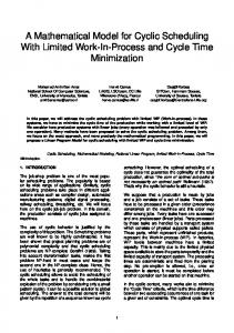
2. Problem Definition and Notation 2.1. Problem Description. Let us consider the following operation process: each manufacturer sends its material requirement plan to the Supply-Hub and corresponding suppliers based on a rolling plan. After that, the Supply-Hub optimizes and arranges the production and distribution activities for each supplier based on the information of production costs and inventory status. Finally, the Supply-Hub implements JIT direct-station distribution according to material requirement plan in each week or day provided by each manufacturer. The illustration of the process is shown in Figure 1. It is worth mentioning that the production information is freely shared among the suppliers, the Supply-Hub and the manufacturers.

The Scientific World Journal

3 Collaborative scheduling model based on the Supply-Hub Material requirement plan in each week or day

Supplier 1

Manufacturer 1 Material requirement plan

Demand information Supply-Hub

Supplier 2 Delivery

Manufacturer 2 JIT delivery

···

···

Supplier n

Manufacturer m

Inventory status report Supplier’s cost information

Figure 1: Multi-suppliers and multi-manufacturers operation mode based on the Supply-Hub.

Note that the coordination scheduling is to implement the JIT distribution of components required by each manufacturer with minimal cost. To achieve this goal, the manufacturer’s distribution lot, the supplier’s production lot, and the distribution frequency should be optimized through integration of the entire supply chain and logistics operation based on the Supply-Hub. In Figure 1, the Supply-Hub provides the service for 𝑚 manufacturers and 𝑛 suppliers. For manufacturer 𝑗, where 𝑗 = 1, 2, . . . , 𝑚, the number of its suppliers is 𝑘𝑗 , where 1 ≤ 𝑘𝑗 ≤ 𝑛. It indicates that the components required by manufacturer 𝑗 are provided by 𝑘𝑗 suppliers. For a certain supplier 𝑖, where 𝑖 = 1, 2, . . . , 𝑛, the number of components required by manufacturer is 𝑙𝑖 , where 1 ≤ 𝑙𝑖 ≤ 𝑚. It implies that the components provided by supplier 𝑖 are required by 𝑙𝑖 manufacturer. Therefore, the multi-suppliers and multi-manufacturers system based on the Supply-Hub considered in our paper is more universal and versatile.

2.2.1. Assumptions. The specific assumptions are as follows. (1) Each supplier provides one kind of the component for a manufacturer, and demand for the component is constant. Note that our results remain unchanged if a certain supplier can provide a variety of components, since it can be actually converted to multiple suppliers and each provides one component. (2) The transportation cost of component 𝑖 required by manufacturer 𝑗 from supplier 𝑖 to the Supply-Hub is composed of a fixed cost 𝐹𝑖𝑗 and a variable cost 𝑉𝑖𝑗 , and the transportation cost from the Supply-Hub to manufacturer 𝑗 also contains a fixed cost 𝐹ℎ,𝑖𝑗 and a variable cost 𝑉ℎ,𝑖𝑗 . (3) The lead time for each level of the supply chain is constant, and it is assumed to be zero without loss of generality. (4) Shortages are not allowed.

2.2. Assumptions and Notations. The Supply-Hub takes charge in the components purchasing and JIT direct-station distribution for 𝑚 manufacturers. Component 𝑖 required by manufacturer 𝑗 is delivered to manufacturer 𝑗 by the SupplyHub at suitable interval 𝑅ℎ,𝑗 , and component 𝑖 from supplier 𝑖 was delivered to the Supply-Hub at regular interval 𝑅𝑖𝑗 . According to the distribution lot to the Supply-Hub, the purchasing lot is determined by supplier 𝑖. Define 𝑤𝑖𝑗 1 ={ 0

if supplier 𝑖 provides component 𝑖 for manufacturer 𝑗 else. (1)

(5) Time horizon is infinite. 2.2.2. Notations. The input parameters and decision variables for manufacturers, the Supply-Hub, and suppliers, are denoted by the subscripts 𝑚, ℎ, and 𝑠, respectively. Manufacturers: 𝑚 is the number of manufacturer; where 𝑗 1, 2, . . . , 𝑚

=

𝑑𝑖𝑗 is the annual demand of manufacturer 𝑗 for the component 𝑖 (units/year); ℎ𝑚,𝑖𝑗 is the manufacturer 𝑗’s holding cost per unit per year for component 𝑖;

4

The Scientific World Journal 𝐴 𝑚,𝑗 is the order cost for manufacturer 𝑗 ($); 𝑇𝑗 is the cycle time (year).

The Supply-Hub: 𝐴 ℎ is the fixed-order/setup cost per cycle for the Supply-Hub; ℎℎ,𝑖 is the Supply-Hub’s holding cost per unit per year for component 𝑖; 𝑀ℎ,𝑗 is an integer multiplier to adjust the order quantity of the Supply-Hub to that of manufacturer 𝑗; 𝐹ℎ,𝑗 is the fixed transportation cost from the SupplyHub to manufacturer 𝑗; 𝑉ℎ,𝑗 is the variable transportation cost from the Supply-Hub to manufacturer 𝑗. Suppliers: 𝑛 is the number of suppliers, where 𝑖 = 1, 2, . . . , 𝑛; 𝐴 𝑠,𝑖 is the order cost for supplier 𝑖; ℎ𝑠,𝑖 is the supplier’s holding cost per unit per unit per year for component 𝑖; 𝑀𝑠,𝑖𝑗 is an integer multiplier to adjust the order quantity of the supplier 𝑖 whose component is required by manufacturer 𝑗 to that of the Supply-Hub; 𝐹𝑠,𝑖𝑗 is the fixed transportation cost for component 𝑖 required by manufacturer 𝑗 from supplier 𝑖 to the Supply-Hub; 𝑉𝑠,𝑖𝑗 is the variable transportation cost for component 𝑖 required by manufacturer 𝑗 from supplier 𝑖 to the Supply-Hub.

3.2. Supply-Hub’s Cost Function. The Supply-Hub manages its upstream manufacturers separately; thus, it places an order for manufacturer 𝑗 every 𝑀ℎ,𝑗 𝑇𝑗 and transports the components to manufacturer 𝑗 every 𝑇𝑗 . The Supply-Hub’s annual cost to satisfy the demand of manufacturer 𝑗 is 𝐶ℎ,𝑗 (𝑀ℎ,𝑗 ) =

𝑛 ℎℎ,𝑖 𝐴ℎ + ∑[ (𝑀ℎ,𝑗 − 1) 𝑑𝑖𝑗 𝑇𝑗 ] 𝑀ℎ,𝑗 𝑇𝑗 𝑖=1 2

+

𝐹ℎ,𝑗 + ∑𝑛𝑖=1 𝑑𝑖𝑗 𝑇𝑗 𝑉ℎ,𝑗 𝑇𝑗

𝐶𝑚,𝑗 =

𝐴 𝑚,𝑗 𝑇𝑗

+

∑𝑛𝑖=1 𝑑𝑖𝑗 𝑇𝑗 ℎ𝑚,𝑖𝑗 2

.

(2)

The annual manufacturers’ cost is the sum of 𝐶𝑚,𝑗 for 𝑚 manufacturers, and it is given as 𝑚

𝑚

𝑗=1

𝑗=1

𝐶𝑚 = ∑ 𝐶𝑚,𝑗 (𝑇𝑗 ) = ∑ (

𝐴 𝑚,𝑗 𝑇𝑗

+

∑𝑛𝑖=1 𝑑𝑖𝑗 𝑇𝑗 ℎ𝑚,𝑖𝑗 2

),

(3)

where 𝑇𝑗 is a decision variable in (3), and the optimal cycle time for manufacturer 𝑗 is 𝑇𝑗∗

=√

2𝐴 𝑚,𝑗

∑𝑛𝑖=1 𝑑𝑖𝑗 ℎ𝑚,𝑖𝑗

.

(4)

In this paper, an optimal value of decision variable will be indicated by an asterisk (∗).

,

where the terms 𝐴 ℎ /𝑀ℎ,𝑗 𝑇𝑗 , ∑𝑛𝑖=1 [(ℎℎ,𝑖 /2)(𝑀ℎ,𝑗 −1)𝑑𝑖𝑗 𝑇𝑗 ], and (𝐹ℎ,𝑗 + ∑𝑛𝑖=1 𝑑𝑖𝑗 𝑇𝑗 𝑉ℎ,𝑗 )/𝑇𝑗 are the Supply-Hub’s annual order cost, the holding cost, and transportation cost for manufacturer 𝑚 which requires component 𝑖 from 𝑛 suppliers. Then the Supply-Hub’s total cost is the sum of (5) for 𝑚 manufacturers, and it is given as 𝑚

𝐶ℎ = ∑𝐶ℎ,𝑗 (𝑀ℎ,𝑗 ) 𝑗=1 𝑚

= ∑{ 𝑗=1

𝑛 ℎℎ,𝑖 𝐴ℎ + ∑[ (𝑀ℎ,𝑗 − 1) 𝑑𝑖𝑗 𝑇𝑗 ] 𝑀ℎ,𝑗 𝑇𝑗 𝑖=1 2

+

𝐹ℎ,𝑗 + ∑𝑛𝑖=1 𝑑𝑖𝑗 𝑇𝑗 𝑉ℎ,𝑗 𝑇𝑗

(6)

},

where 𝑀ℎ,𝑗 is a decision variable in (6), and the Supply-Hub’s optimal cycle time for manufacturer 𝑗 is

3. Model Formulation 3.1. Manufacturer’s Cost Function. Manufacturer 𝑗 orders ∑𝑛𝑖=1 𝑑𝑖𝑗 𝑇𝑗 units from the Supply-Hub every 𝑇𝑗 . The total annual cost for a manufacturer is the sum of the annual order cost, 𝐴 𝑚,𝑗 /𝑇𝑗 , and the annual holding cost, ∑𝑛𝑖=1 𝑑𝑖𝑗 𝑇𝑗 ℎ𝑚,𝑖𝑗 /2. The annual cost function for manufacturer 𝑗 is given by

(5)

𝑀ℎ,𝑗 =

2𝐴 1 √ 𝑛 ℎ . 𝑇𝑗 ∑𝑖=1 ℎℎ,𝑖 𝑑𝑖𝑗

(7)

3.3. Supplier’s Cost Function. The Supply-Hub has 𝑛 suppliers to provide all 𝑛 components. When manufacturer 𝑗 places an order of size ∑𝑛𝑖=1 𝑑𝑖𝑗 𝑇𝑗 with the Supply-Hub every 𝑇𝑗 and as discussed above, the Supply-Hub determines its order quantity 𝑀ℎ,𝑗 𝑑𝑖𝑗 𝑇𝑗 for the supplier 𝑖. In order to fulfill the demand of manufacturer 𝑗, the order of size 𝑀ℎ,𝑗 𝑑𝑖𝑗 𝑇𝑗 will be placed by the Supply-Hub, and shipment will occur every 𝑀ℎ,𝑗 𝑇𝑗 . The annual cost for supplier 𝑖 is written as 𝑚

𝐶𝑠,𝑖 (𝑀𝑠,𝑖𝑗 ) = ∑ [ 𝑗=1

ℎ𝑠,𝑖 𝑀ℎ,𝑗 𝐴 𝑠,𝑖 + (𝑀𝑠,𝑖𝑗 − 1) 𝑑𝑖𝑗 𝑇𝑗 𝑀𝑠,𝑖𝑗 𝑀ℎ,𝑗 𝑇𝑗 2 +

𝐹𝑠,𝑖𝑗 + 𝑉𝑠,𝑖𝑗 𝑀ℎ,𝑗 𝑇𝑗 𝑑𝑖𝑗 𝑀ℎ,𝑗 𝑇𝑗

], (8)

where the terms 𝐴 𝑠,𝑖 /𝑀𝑠,𝑖𝑗 𝑀ℎ,𝑗 𝑇𝑗 , (ℎ𝑠,𝑖 𝑀ℎ,𝑗 /2)(𝑀𝑠,𝑖𝑗 −1)𝑑𝑖𝑗 𝑇𝑖𝑗 , and (𝐹𝑠,𝑖𝑗 + 𝑉𝑠,𝑖𝑗 𝑀ℎ,𝑗 𝑇𝑗 𝑑𝑖𝑗 )/𝑀ℎ,𝑗 𝑇𝑗 are, respectively, the annual

The Scientific World Journal

5

order cost, holding cost, and transportation cost for supplier 𝑖 to meet the annual demand for components required by the Supply-Hub. Then the collective annual cost for 𝑛 suppliers is given as

4. Supply Chain Coordination The annual supply chain’s cost is determined by summing (3), (6), and (9) to obtain 𝐶csc = 𝐶𝑚 + 𝐶ℎ + 𝐶𝑠

𝑛

𝑚

𝐶𝑠 = ∑𝐶𝑠,𝑖 (𝑀𝑠,𝑖𝑗 ) 𝑖=1 𝑛 𝑚

= ∑∑ [ 𝑖=1 𝑗=1

= ∑(

𝑇𝑗

𝑗=1

ℎ𝑠,𝑖 𝑀ℎ,𝑗 𝐴 𝑠,𝑖 + (𝑀𝑠,𝑖𝑗 − 1) 𝑑𝑖𝑗 𝑇𝑗 𝑀𝑠,𝑖𝑗 𝑀ℎ,𝑗 𝑇𝑗 2 +

𝐴 𝑚,𝑗

𝐹𝑠,𝑖𝑗 + 𝑉𝑠,𝑖𝑗 𝑀ℎ,𝑗 𝑇𝑗 𝑑𝑖𝑗 𝑀ℎ,𝑗 𝑇𝑗

𝑚

+∑{ 𝑗=1

+

(9) 𝑛 𝑚

2𝐴 𝑠,𝑖 1 . √ 𝑀ℎ,𝑗 𝑇𝑗 𝑑𝑖𝑗

2

)

+ ∑∑ [ 𝑖=1 𝑗=1

𝐹ℎ,𝑗 + ∑𝑛𝑖=1 𝑑𝑖𝑗 𝑇𝑗 𝑉ℎ,𝑗 𝑇𝑗

}

ℎ𝑠,𝑖 𝑀ℎ,𝑗 𝐴 𝑠,𝑖 + (𝑀𝑠,𝑖𝑗 − 1) 𝑑𝑖𝑗 𝑇𝑗 𝑀𝑠,𝑖𝑗 𝑀ℎ,𝑗 𝑇𝑗 2 +

𝑀𝑠,𝑖𝑗 =

∑𝑛𝑖=1 𝑑𝑖𝑗 𝑇𝑗 ℎ𝑚,𝑖𝑗

𝑛 ℎℎ,𝑖 𝐴ℎ + ∑[ (𝑀ℎ,𝑗 − 1) 𝑑𝑖𝑗 𝑇𝑗 ] 𝑀ℎ,𝑗 𝑇𝑗 𝑖=1 2

],

where 𝑀𝑠,𝑖𝑗 is a decision variable in (9), and the supplier 𝑖’s optimal cycle time for manufacturer 𝑗 is

+

𝐹𝑠,𝑖𝑗 + 𝑉𝑠,𝑖𝑗 𝑀ℎ,𝑗 𝑇𝑗 𝑑𝑖𝑗 𝑀ℎ,𝑗 𝑇𝑗

]. (11)

(10)

3.4. Solution Procedures with Decentralized Decision (1) Each manufacturer 𝑗 determines its optimal cycle time, 𝑇𝑗∗ = √2𝐴 𝑚,𝑗 / ∑𝑛𝑖=1 𝑑𝑖𝑗 ℎ𝑚,𝑖𝑗 , where 𝑖 = 1, 2, . . . , 𝑛,𝑗 = 1, 2, . . . , 𝑚. Then the collective annual manufacturers’ cost 𝐶𝑚 is computed from (3).

(2) The value of 𝑇𝑗∗ is input into (7), 𝑀ℎ,𝑗 = (1/𝑇𝑗∗ ) √2𝐴 ℎ / ∑𝑛𝑖=1 ℎℎ,𝑖 𝑑𝑖𝑗 . If 𝐶ℎ,𝑗 (⌈𝑀ℎ,𝑗 ⌉) ≥ 𝐶ℎ,𝑗 (⌊𝑀ℎ,𝑗 ⌋), ∗ ∗ = ⌊𝑀ℎ,𝑗 ⌋. Or else 𝑀ℎ,𝑗 = ⌈𝑀ℎ,𝑗 ⌉. then 𝑀ℎ,𝑗 This should be repeated for 𝑚 manufacturers, after which the collective Supply-Hub’s annual cost, 𝐶ℎ = ∑𝑚 𝑗=1 𝐶ℎ,𝑗 , is computed from (6). ∗ are input into (8), and (3) The values of 𝑇𝑗∗ and 𝑀ℎ,𝑗 (8) is minimized by searching the optimal value of ∗ = 𝑀𝑠,𝑖𝑗 . If 𝐶𝑠,𝑖 (⌈𝑀𝑠,𝑖𝑗 ⌉) ≥ 𝐶𝑠,𝑖 (⌊𝑀𝑠,𝑖𝑗 ⌋), then 𝑀𝑠,𝑖𝑗 ∗ ⌊𝑀𝑠,𝑖𝑗 ⌋, or else 𝑀𝑠,𝑖𝑗 = ⌈𝑀𝑠,𝑖𝑗 ⌉. This may be repeated for 𝑚 ⋅ 𝑛 times because the component 𝑖 provided by supplier 𝑖 may be required by manufacturer 𝑗, where 𝑖 = 1, 2, . . . , 𝑛, 𝑗 = 1, 2, . . . , 𝑚. Then the collective supplier’s annual cost 𝐶𝑠 is computed from (9). ∗ ∗ , and 𝑀𝑠,𝑖𝑗 for each side (4) The value of optimal 𝑇𝑗∗ , 𝑀ℎ,𝑗 should be recorded and the total supply chain cost for the case of no coordination is 𝐶𝑛𝑠𝑐 = 𝐶𝑚 + 𝐶ℎ + 𝐶𝑠 , which can be obtained after the above three steps.

This is a centralized decision-making process, in which the Supply-Hub tries to schedule and optimize each decision variable for the entire supply chain. It is general and practical that the Supply-Hub takes charge of distribution frequency and purchasing frequency for the suppliers and the manufacturers, respectively. Note that (11) is convex and differentiable over 𝑇𝑗 , where 3 𝜕2 𝐶csc /𝜕2 𝑇𝑗 = ∑𝑚 𝑗=1 [(2/𝑇𝑗 )(𝐴 𝑚,𝑗 + (𝐴 ℎ /𝑀ℎ,𝑗 ) + 𝐹ℎ,𝑗 + ∑𝑛𝑖=1 (𝐴 𝑠,𝑖 /𝑀𝑠,𝑖𝑗 𝑀ℎ,𝑗 ) + ∑𝑛𝑖=1 (𝐹𝑠,𝑖𝑗 /𝑀ℎ,𝑗 ))] > 0 for every 𝑇𝑗 > 0, since 𝐴 𝑚,𝑗 , 𝐴 ℎ , 𝐹ℎ,𝑗 , 𝐹𝑠,𝑖𝑗 , 𝐴 𝑠,𝑖 , 𝑀ℎ,𝑗 , 𝑀𝑠,𝑖𝑗 > 0. Therefore at a particular set of values for 𝑀𝑠,𝑖𝑗 ≥ 1 and 𝑀ℎ,𝑗 ≥ 1, where 𝑀𝑠,𝑖𝑗 and 𝑀ℎ,𝑗 are integer, 𝑖 = 1, 2, . . . , 𝑛, 𝑗 = 1, 2, . . . , 𝑚, the first derivative of (11) should be set to zero and the optimal 𝑇𝑗∗ was obtained. Consider

𝑇𝑗∗ = (2 [𝐴 𝑚,𝑗 +

𝑛 𝑛 𝐹 𝐴 𝑠,𝑖 𝐴ℎ 𝑠,𝑖𝑗 +∑ + 𝐹ℎ,𝑗 + ∑ ] 𝑀ℎ,𝑗 𝑖=1 (𝑀𝑠,𝑖𝑗 𝑀ℎ,𝑗 ) 𝑖=1 𝑀ℎ,𝑗

𝑛

𝑛

𝑖=1

𝑖=1

× (∑𝑑𝑖𝑗 ℎ𝑚,𝑖𝑗 + (𝑀ℎ,𝑗 − 1) ∑ℎℎ,𝑖 𝑑𝑖𝑗 + 𝑀ℎ,𝑗 1/2 𝑛

−1

× ∑ (𝑀𝑠,𝑖𝑗 − 1) 𝑑𝑖𝑗 ) )

.

𝑖=1

(12) 4.1. Complexity Analysis for This Problem. The complexities of solving this problem are analyzed as follows. The optimal 𝑇𝑗 , 𝑀ℎ,𝑗 , and 𝑀𝑠,𝑖𝑗 should be obtained to minimize the supply chain’s cost 𝐶csc , where 𝑖 = 1, 2, . . . , 𝑛, 𝑗 = 1, 2, . . . , 𝑚. If

6

The Scientific World Journal

a certain group of solution to this problem was proved NPcomplete, then the whole group of solutions to this problem must be NP-complete. Taking supplier 1 as the representative case, whose problem is to minimize 𝐶csc (𝑀𝑠,1𝑗 , 𝑀ℎ,𝑗 , 𝑇𝑗 | 𝑗 = 1, 2, . . . , 𝑚). We define this problem as 𝑃. If the problem 𝑃 can be proved to equal partition problem, then the problem 𝑃 is NP-complete. Partition Problem. Given the positive integer 𝑛, 𝐵, and a group of positive integers 𝐺 = {𝑥1 , 𝑥2 , . . . , 𝑥𝑛 }, then ∑𝑛𝑖=1 𝑥𝑖 = 2𝐵, can 𝐺 be divided into group 𝐺1 and 𝐺−𝐺1 to make ∑𝑥𝑖 ∈𝐺𝑖 𝑥𝑖 = ∑𝑥𝑖 ∈𝐺−𝐺𝑖 𝑥𝑖 = 𝐵. Lemma 1. Partition is NP-complete; see Garey and Johnson [21]. Proposition 2. The problem 𝑃 is NP-complete. Proof. We should transform the problem 𝑃 to partition. Let the sets 𝑇, 𝑀ℎ , 𝑀𝑠,1 , with |𝑇| = |𝑀ℎ | = |𝑀𝑠,1 | = 𝑚, and 𝑊 ⊆ 𝑇 × 𝑀ℎ × 𝑀𝑠,1 be an arbitrary instance of problem 𝑃. Let the elements of these sets be denoted by 𝑇 = {𝑇1 , 𝑇2 , . . . , 𝑇𝑚 }, 𝑀ℎ = {𝑀ℎ,1 , 𝑀ℎ,2 , . . . , 𝑀ℎ,𝑚 }, 𝑀𝑠,1 = {𝑀𝑠,11 , 𝑀𝑠,12 , . . . , 𝑀𝑠,1𝑚 }, and 𝑊 = {𝑊1 , 𝑊2 , . . . , 𝑊𝑞 }, where |𝑊| = 𝑞. We should construct a set 𝐺 and a size 𝑠 (𝑎) ∈ 𝑍+ for each 𝑎 ∈ 𝐺, such that 𝐺 contains a subset 𝐺1 satisfying ∑ 𝑠 (𝑎) =

∑ 𝑠 (𝑎) .

𝑎∈𝐺1

𝑎∈𝐺−𝐺1

(13)

The set 𝐺 will contain a total of 𝑞 + 2 elements and will be constructed in two steps. The first 𝑞 elements of 𝐺 are {𝑎𝑘 : 1 ≤ 𝑘 ≤ 𝑞}, where the element 𝑎𝑘 is associated with the group 𝑊𝑘 ∈ 𝑊. The size 𝑠 (𝑎𝑘 ) of 𝑎𝑘 will be specified by giving its binary representation, in terms of a string of 0’s and 1’s divided into 3𝑚 “zones” of 𝑝 = [log2 (𝑞 + 1)] bits each. Then each 𝑠 (𝑎𝑘 ) can be expressed in binary with no more than 3𝑝𝑚 bits; it is clear that 𝑠 (𝑎𝑘 ) can be constructed from the given problem 𝑃 instance in polynomial time; see Garey and Johnson [21]. If we sum up all elements in any zone, the total can never exceed 𝑞 = 2𝑝 − 1. Therefore, in adding up ∑𝑎∈𝐺1 𝑠 (𝑎) for any subset 𝐺1 ∈ {𝑎𝑘 : 1 ≤ 𝑘 ≤ 𝑞}, there will never be any “carries” 𝑝𝑠 from one zone to the next. If we define 𝐵 = ∑3𝑚−1 𝑠=0 2 , then any subset 𝐺1 ∈ {𝑎𝑘 : 1 ≤ 𝑘 ≤ 𝑞} will satisfy ∑ 𝑠 (𝑎) = 𝐵. 𝑎∈𝐺1

(14)

The last two elements are denoted by 𝑏1 and 𝑏2 ; that is, 𝑞

𝑠 (𝑏1 ) = 2 ∑ 𝑠 (𝑎𝑘 ) − 𝐵, 𝑘=1 𝑞

𝑠 (𝑏2 ) = ∑ 𝑠 (𝑎𝑘 ) + 𝐵. 𝑘=1

(15)

Now suppose we have a subset 𝐺1 ∈ 𝐺 such that ∑ 𝑠 (𝑎) = 𝑎∈𝐺1

∑ 𝑠 (𝑎) .

(16)

𝑎∈𝐺−𝐺1 𝑞

Then both of these sums must be equal to 2 ∑𝑘=1 𝑠 (𝑎𝑘 ), and one of the two sets, 𝐺1 or 𝐺 − 𝐺1 , contains 𝑏1 but not 𝑏2 . It follows that the remaining elements of that set form a subset of {𝑎𝑘 : 1 ≤ 𝑘 ≤ 𝑞} whose sizes sum to 𝐵. Therefore the problem 𝑃 can be transformed to partition, and Proposition 2 is proved. 4.2. Solution Procedure. Since the coordination scheduling problem of multiple suppliers and multiple manufacturers based on the Supply-Hub is NP-complete, the solution may be very complex. Therefore, the auto-adapted differential evaluation algorithm will be proposed to solve this problem by this paper. The differential evolution algorithm put forward by Rainer Storn and Kenneth Price in 1997 is for meta-heuristic global optimization based on population evolutionary and the real coding, which is originally used to solve the Chebyshev polynomials. As to more complex global optimization problems of continuous space, such as non-linear and nondifferentiable problems even without function expression, the differential evaluation algorithm has a better global optimization ability and higher convergence performance with simple operation, less controlling parameters, and better robustness, compared to genetic algorithms, particle swarm optimization, simulated annealing, tabu search, and so forth. The evolution process of differential evaluation algorithm is similar to genetic algorithms, including population initialization, variation, hybridization, and selection. But the main differences between these two algorithms are that the process of variation is before hybridization for differential evolution algorithm, and evaluation of population depends on comparisons with testing chromosome and target chromosome. As a result, the solution procedure of coordination scheduling problem can be proposed as follows. 4.2.1. Population Initialization. Let 𝑔 stands for the generation of population 𝑃𝑔 , and the scale of population is NP; that 𝑔 𝑔 is, 𝑃𝑔 = {𝑥𝑖∗ }, where 𝑖∗ = 1, 2, . . . , NP. 𝑥𝑖∗ is a feasible solution 𝑔 of the population 𝑃 , which is composed of a vector of 𝐷 𝑔 𝑔 𝑔 𝑔 variables, that is 𝑥𝑖∗ = (𝑥𝑖∗ 1 , 𝑥𝑖∗ 2 , . . . , 𝑥𝑖∗ 𝐷). As for our scheduling problem, 𝐷 is the number of 𝑔 𝑔 𝑔 𝑔 decision variables. Let 𝑥𝑖∗ = (𝑥𝑖∗ 1 , 𝑥𝑖∗ 2 , . . . , 𝑥𝑖∗ 𝐷) = (𝑀ℎ,1 , 𝑀ℎ,2 , . . . , 𝑀ℎ,𝑚 ; 𝑀𝑠,11 ,𝑀𝑠,21 , . . . , 𝑀𝑠,𝑛1 ; 𝑀𝑠,12 , 𝑀𝑠,22 , . . . ,𝑀𝑠,𝑛2 ; . . . ; 𝑀𝑠,1𝑚 , 𝑀𝑠,2𝑚 , . . . , 𝑀𝑠,𝑛𝑚 ). 𝑔=0 Initialize the population, set 𝑔 = 0, and 𝑥𝑖∗ 𝑗∗ = 𝑙𝑗∗ + rand𝑗∗ ⋅ (ℎ𝑗∗ − 𝑙𝑗∗ ). Where rand𝑗∗ is a real number generated by uniform random distribution in [0, 1), ℎ𝑗∗ and 𝑙𝑗∗ are the upper and lower boundaries of individual variables, which are randomly distrusted real numbers. 𝑔+1

= 4.2.2. Variations. The interim of individuals, V𝑖∗ 𝑔+1 𝑔+1 𝑔+1 (V𝑖∗ 1 , V𝑖∗ 2 , . . . , V𝑖∗ 𝐷 ), should be generated after any individual 𝑔 𝑔 𝑥𝑖∗ is determined in population 𝑃𝑔 , where the number of 𝑥𝑖∗

The Scientific World Journal

7

is 𝑟 (3 ≤ 𝑟 ≤ NP). Let individual set Ω = {𝜉1 , 𝜉2 , . . . , 𝜉𝑟 } and 𝑔+1 after variation the interim individuals V𝑖∗ are 𝑔+1

V𝑖∗ = 𝜉1 + 𝐹 ⋅ [(𝜉2 − 𝜉3 ) + (𝜉3 − 𝜉4 ) + ⋅ ⋅ ⋅ + (𝜉𝑟−1 − 𝜉𝑟 )] , (17) where 𝐹 is a differential scale factor. As for our scheduling 𝑔+1 problem, the interim individuals V𝑖∗ should be rounded to the nearest integer since decision variables 𝑀𝑠,𝑖𝑗 and 𝑀ℎ,𝑗 must be positive integers, where 𝑖 = 1, 2, . . . , 𝑛, 𝑗 = 1, 2, . . . , 𝑚. 𝑔+1

4.2.3. Hybridization. The interim individuals V𝑖∗ should 𝑔 be crossed with current individuals 𝑥𝑖∗ in probability CR, where CR ∈ [0, 1]. The proper individuals can be gener𝑔+1 𝑔+1 𝑔+1 𝑔+1 ated after hybridization. Set 𝑈𝑖∗ = (𝑢𝑖∗ 1 , 𝑢𝑖∗ 2 , . . . , 𝑢𝑖∗ 𝐷 ). 𝑔+1 𝑔+1 𝑔+1 𝑢𝑖∗ 1 , 𝑢𝑖∗ 2 , . . . , 𝑢𝑖∗ 𝐷 is a feasible solution of decision variables. Consider 𝑔+1 𝑢𝑖∗ 𝑗∗

𝑔+1

V∗ ∗ = { 𝑖𝑔 𝑗 𝑥𝑖∗ 𝑗∗

rand𝑖∗ 𝑗∗ ≤ CR or 𝑗 = rand (𝑖) else

(18)

(𝑖∗ = 1, 2, . . . , NP; 𝑗∗ = 1, 2, , 𝐷) , where CR is the cross rate. The larger the CR is, the more the 𝑔+1 𝑔+1 𝑢𝑖∗ 𝑗∗ can be influenced by V𝑖∗ 𝑗∗ , which leads the algorithm to faster convergence with local optimization. In order to increase the performance of differential evolution algorithm, the auto-adapted cross rate was proposed. Let CR (𝐺𝑡=0 ) = CRmax . When the differential evolution algorithm in the fixed loop of evaluation does not improve significantly, CR can be automatically adapted according to CR (𝐺𝑡+1 ) = {

0.95CR (𝐺𝑡 ) if 0.95CR (𝐺𝑡 ) ≥ CRmin (19) CRmin else,

where CRmax and CRmin are the maximum and minimum crossover probabilities, respectively. 𝐺 is the total evaluation number. 𝐺𝑡+1 stands for evaluation value in cycle 𝑡 + 1. The auto-adapted change of CR can improve performance of the whole algorithm and enhance the ability of global optimization algorithms. 𝑔+1

4.2.4. Selection. The fitness of candidate individual 𝑈𝑖∗ should be evaluated after hybridization. The candidate indi𝑔+1 vidual 𝑈𝑖∗ can be determined whether it replaces the current 𝑔 individuals 𝑥𝑖∗ or not according to 𝑔+1

𝑥𝑖∗ = {

𝑔+1

𝑈𝑖∗ 𝑔 𝑥𝑖∗

𝑔+1

𝑔

if 𝐶csc (𝑇, 𝑈𝑖∗ ) ≤ 𝐶csc (𝑇, 𝑥𝑖∗ ) else,

(20)

where 𝐶csc (⋅) is the fitness function, which corresponds to the total cost of (11), and 𝑇 = {𝑇1 , 𝑇2 , . . . , 𝑇𝑚 }, where 𝑇𝑗∗ (𝑗 = 1, 2, . . . , 𝑚) can be calculated from (12). The process should be repeated and the best solution should be output 𝑔+1 corresponding to 𝑥𝑖∗ and 𝑇.

Table 1: Stability analysis of the auto-adapted DE algorithm. 𝑚 9 7 5 3 3 3 3

𝑛 10 10 10 10 8 6 4

Best value 38408 30160 21618 12786 10524 8267 5206

Worst value 38633 30382 21783 12937 10666 8390 5418

Mean 38504 30304 21706 12855 10597 8311 5342

Standard deviation 42 38 37 31 27 26 31

5. Numerical Analysis 5.1. Parameters Setting. Numerical experiments are conducted to examine the computational effectiveness and efficiency of the proposed auto-adapted differential evaluation algorithm by comparing it with the method of decentralized decision. The parameters of the auto-adapted DE algorithm are as follows: 𝐷 = 𝑚+𝑚∗𝑛, NP = 𝐷, 𝐹min = 0.2, 𝐹max = 0.6, CRmin = 0.2, CRmax = 0.8, and the maximum number of iterations GenM is set at 500 when 𝑚 = 10 and 𝑛 = 9, 7, 5; GenM is set at 400 when 𝑛 = 3 and 𝑚 = 10, 8; GenM is set at 300 when 𝑛 = 3 and 𝑚 = 6, 4. The detailed settings for each test problem are as follows. 𝐴 𝑠,𝑖 is selected 𝑈 [200, 300].

from

uniform

distribution

ℎ𝑠,𝑖 is selected from uniform distribution 𝑈 [1, 3]. 𝐹𝑠,𝑖𝑗 = 30 and 𝑉𝑠,𝑖𝑗 is selected from uniform distribution 𝑈 [10, 20]. 𝐴 ℎ = 50, ℎℎ,𝑖 = 𝛼1 ⋅ ℎ𝑠,𝑖 , 𝛼1 = 0.8. 𝐹ℎ,𝑗 = 5 and 𝑉ℎ,𝑗 is selected from uniform distribution 𝑈 [1, 6]. If 𝑤𝑖𝑗 = 1, 𝑑𝑖𝑗 is selected from uniform distribution 𝑈 [10, 20]; otherwise, 𝑑𝑖𝑗 = 0. ℎ𝑚,𝑗 = 𝛼2 ⋅ (max ℎ𝑠,𝑖 ), 𝛼2 = 3. 𝐴 𝑚 is selected from uniform distribution 𝑈 [20, 30]. 5.2. Comparative Evaluations. Figures 2, 3, and 4 show the evolution of best solution under 3 different cases, respectively, and we run the proposed auto-adapted DE algorithm under every case for 100 times and calculate its best solutions, worst solutions, means, and standard deviations; the result is shown in Table 1. The results of the auto-adapted DE algorithm and those of the method of decentralized decision are shown in Tables 2 and 3. In Table 2, we assume 𝑛 = 10 and 𝑚 = 9, 7, 5, 3. In Table 3, we assume 𝑚 = 3 and 𝑛 = 10, 8, 6, 4. In both the two tables, C𝑠,𝑖 denotes the cost of supplier 𝑖; Cℎ denotes the cost of Supply-Hub; C𝑚,𝑗 denotes the cost of manufacturer 𝑗; and Csc denotes the cost of supply chain. Table 4 shows the difference of every cost item in the context of joint decision and decentralized decision when 𝑛 = 10. Table 5 shows the difference of every cost item in context of joint decision and decentralized decision when 𝑚 = 3. From Figures 2, 3, and 4, it can be seen that the autoadapted DE algorithm is convergent under these 3 cases; in

0.24 0.28 0.23 0.28 0.23 0.24 0.26 0.26 0.25

4442634074 3453335403 2402533453 2034723442 4053333532 4343634540 3333034533 3333524360 3355033444

3332323043 3332423403 3302423553 2033533453 3032334453 4343442350 4333024543

3232222043 3232322302 2302322332 3022322332 2022222332

3232322052 3232322302 2302222542

6 5 7 6 7 6 6 6 6

8 5 7 6 6 6 8

7 8 8 8 10

8 7 9

9

7

5

3

0.26 0.29 0.22

0.29 0.26 0.25 0.27 0.24

0.24 0.33 0.23 0.27 0.28 0.27 0.21

𝑇𝑗

𝑀𝑠,𝑖𝑗

𝑀ℎ,𝑗

𝑚

2392 1696.5 2139 2962 2333 2007 2464 2574 2193 2147 1600 995.5 1360.5 2170 1992 1429 1676 1556 1412 1754.5 955 996 617 1370 1294 968.5 1042 761 713 1016

3021 2405 2921 3858 2803 2670 3273.5 3397 2800 2465

Joint decision 𝐶𝑠,𝑖

2330

3973

5157

6177

𝐶ℎ

29820

21172

12786

250 250 270 262 222

245 256 266

37968

𝐶sc

243 269 267 262 230 230 255

243 254 266 264 221 226 256 241 206

𝐶𝑚,𝑗

3 3 3

3 3 3 3 4

3 3 3 3 4 3 3

3 3 3 3 4 3 3 3 3

𝑀ℎ,𝑗

7675655096 8676756805 6705756985

7675655096 8676756805 6705756985 6067755795 5054656774

7675655096 8676756805 6705756985 6067755795 5054656774 6776965890 6566056786

0.23 0.21 0.21

0.23 0.21 0.21 0.22 0.2

0.23 0.21 0.21 0.22 0.2 0.21 0.23

0.23 0.21 0.21 0.22 0.2 0.21 0.23 0.21 0.21 2638 1895 2355 3280 2517 2303 2719 2756 2365 2365 1836 1151 1544 2457 2202 1704 1937 1721 1566 2017 1100.5 1151 702 1552 1377 1144 1204 834 776.5 1181

3334 2647 3151 4184 2939 3012 3545 3638 3032 2718

Decentralized decision 𝑇𝑗 𝐶𝑠,𝑖

7675655096 8676756805 6705756985 6067755795 5054656774 6776965890 6566056786 7 6 7 6 7 5 6 8 10 0 7 7 7 6 0 6 6 9 10 6

𝑀𝑠,𝑖𝑗

Table 2: The result of joint decision and decentralized decision when 𝑛 = 10.

2039

3483

4779

5801

𝐶ℎ

243 245 266

243 245 266 258 219

243 245 266 258 219 224 253

243 245 266 258 219 224 253 234 203

𝐶𝑚,𝑗

13814

22848

31680

40147

𝐶sc

8 The Scientific World Journal

𝑀𝑠,𝑖𝑗

3232322052 3232322302 2302222542

22222220 32223222 22022223

322222 323232 220221

2222 2222 1201

𝑀ℎ,𝑗

8 7 9

8 8 8

7 6 7

6 6 8

𝑛

10

8

6

4

Joint decision 𝐶𝑠,𝑖 955 996 617 1370 0.26 1294 0.29 968.5 0.22 1042 761 713 1016 939.5 979 600 0.3 1361 0.28 1234 0.28 963 1031 742 948 980 0.3 610 0.3 1365 0.4 1232 947 892 0.4 966 0.4 594 0.5 1304

𝑇𝑗

1057

1570

1980.5

2330

𝐶ℎ

162 155 154

204.5 205 205.5

223 234 236

245 256 266

𝐶𝑚,𝑗

5284

8267

10524

12786

𝐶sc

3 3 3

3 3 3

3 3 3

3 3 3

𝑀𝑠,𝑖𝑗

Decentralized decision 𝑇𝑗 𝐶𝑠,𝑖 1100.5 1151 702 1552 7675655096 0.23 1377 8676756805 0.21 1144 6705756985 0.21 1204 834 776.5 1181 1085 1134.5 693 65646450 0.25 1536 75766468 0.23 1362 56046456 0.24 1127 1187 824 1066 1116 656454 0.28 682 656464 0.26 1512 550454 0.28 1344 1105 1030 4453 0.35 1079 5344 0.34 661.5 3403 0.37 1470 𝑀𝑠,𝑗

Table 3: The result of joint decision and decentralized decision when 𝑚 = 3.

895

1380

1703.5

2039

𝐶ℎ

159.5 152 150

202 199 200

220 229 234

243 245 266

𝐶𝑚,𝑗

5597

8806

11335

13814

𝐶sc

The Scientific World Journal 9

10

The Scientific World Journal Table 4: The difference of every cost item when 𝑛 = 10.

×104 4.05

Best solution

4 3.95 3.9 3.85 3.8 3.75

0

50

100

150

200 250 300 Generation

350

400

450

500

Figure 2: The evolution of best solution when 𝑚 = 9, 𝑛 = 10. ×104

1.38 1.36

Best solution

1.34

1.28 1.26

0

100

50

150

200

250

300

350

400

Generation

Figure 3: The evolution of best solution when 𝑚 = 3, 𝑛 = 10. 9000 8900 8800 8700 8600 8500 8400 8300 8200

9 −9.4% −9.1% −7.3% −7.8% −4.6% −11.4% −7.6% −6.6% −7.7% −9.3% 0% 3.7% 0% 2.3% 0.9% 0.9% 1.2% 3% 1.5% 6.5% −5.4%

7 −9.3% −10.4% −9.2% −9.7% −7.3% −12.9% −9.4% −6.6% −7.3% −9.2% 0% 9.8% 0.4% 1.6% 5% 2.7% 0.8%

5 −12.9% −13.5% −11.9% −11.7% −9.5% −16.1% −13.5% −9.6% −9.8% −13% 2.9% 2% 1.5% 1.6% 1.4%

3 −13.2% −13.5% −12.1% −11.7% −6% −15.3% −13.5% −8.8% −8.1% −14% 0.8% 4.5% 0%

7.9% −5.9%

14.1% −7.3%

14.3% −7.4%

Table 5: The change of every cost item when 𝑚 = 3.

1.32 1.3

Best solution

𝑚 Δ𝐶𝑠1 Δ𝐶𝑠2 Δ𝐶𝑠3 Δ𝐶𝑠4 Δ𝐶𝑠5 Δ𝐶𝑠6 Δ𝐶𝑠7 Δ𝐶𝑠8 Δ𝐶𝑠9 Δ𝐶𝑠10 Δ𝐶𝑚1 Δ𝐶𝑚2 Δ𝐶𝑚3 Δ𝐶𝑚4 Δ𝐶𝑚5 Δ𝐶𝑚6 Δ𝐶𝑚7 Δ𝐶𝑚8 Δ𝐶𝑚9 Δ𝐶ℎ Δ𝐶𝑠𝑐

0

50

100

150 Generation

200

250

300

Figure 4: The evolution of best solution when 𝑚 = 3, 𝑛 = 6.

𝑛 Δ𝐶𝑚1 Δ𝐶𝑚2 Δ𝐶𝑚3 Δ𝐶𝑠1 Δ𝐶𝑠2 Δ𝐶𝑠3 Δ𝐶𝑠4 Δ𝐶𝑠5 Δ𝐶𝑠6 Δ𝐶𝑠7 Δ𝐶𝑠8 Δ𝐶𝑠9 Δ𝐶𝑠10 Δ𝐶ℎ Δ𝐶𝑠𝑐

10 0.8% 4.5% 0% −13.2% −13.5% −12.1% −11.7% −6% −15.3% −13.5% −8.8% −8.1% −14% 14.3% −7.4%

8 1.4% 2.2% 0.9% −13.4% −13.7% −13.4% −11.4% −9.4% −14.6% −13.1% −10%

6 1.2% 3% 2.8% −11.1% −12.2% −10.6% −9.7% −8.3% −14.3%

4 1.3% 2% 2.7% −13.4% −10.5% −10.3% −11.3%

16.3% −7.2%

13.8% −6.1%

18.1% −5.6%

fact, the algorithm is convergent under all these 7 cases in our numerical experiment; we only show the 3 figures due to the limited space. From Table 1 we can see that even under the case 𝑚 = 9 and 𝑛 = 10, the standard deviation is relatively small, so we can conclude that the auto-adapted DE algorithm is stable. From Tables 2, 3, 4, and 5, we can obtain some conclusions as follows. (1) When suppliers, the Supply-Hub, and manufacturers make decisions as a whole, the total cost of supply

The Scientific World Journal chain can be reduced compared to the corresponding cost when they make decisions decentralized. Tables 4 and 5 reveal that the total cost of supply chain can be reduced by 5.4% at least, 7.4% at most. (2) When suppliers, the Supply-Hub, and manufacturers make decisions centralized, every supplier’s cost decreases, but the Supply-Hub’s cost and every manufacturer’s cost increases, and the decreased cost is more than the increased one, so the total cost of supply chain can be reduced. We can see that the SupplyHub’s cost increases greatly in context of centralized decision-making from Tables 4 and 5, so the operator of the Supply-Hub may be not willing to make decisions centralized. In fact, suppliers always sell their products to the manufacturer on consignment under Supply-Hub mode. The inventory holding cost is paid by suppliers when their products are stored in the Supply-Hub, as every supplier’s cost decreases greatly on the condition of centralized decision-making, so they are willing to pay the increased inventory holding cost. (3) The Supply-Hub’s distribution interval and every supplier’s distribution interval increase under centralized decision-making compared to the results obtained in the case of decentralized decision-making, but for supplier’s order interval, some increase and others decrease. From Tables 2 and 3, it can be seen that every supplier’s distribution interval and 𝑀ℎ,𝑗 increase in the context of centralized decision-making, so the Supply-Hub’s distribution interval for every manufacturer also increases under this case. (4) From Table 2, it can be seen that in case of decentralized decision-making, all the suppliers’ and SupplyHub’s decisions remain the same as the number of manufacturer increases, but under centralized decision-making, their decisions change as the number of manufacturer increases. This is because in the context of centralized decision-making, every decision maker considers the influence of his decision on others, and they optimize the whole supply chain collaboratively. Therefore, as the number of manufacturer increases, all the suppliers and the Supply-Hub change their optimal decisions.

6. Conclusions This paper examines the collaborative scheduling model for the Supply-Hub consists of multiple suppliers and multiple manufacturers. We describe the basic operational process of the Supply-Hub and formulate the basic decision models. Given two different scenarios of decentralized system and collaborative system, we first consider the case that the Supply-Hub, the suppliers, and the manufacturers operate separately in their delivery quantities, production quantities, and order quantities. We next consider the collaborative mechanism, in which the Supply-Hub makes the entire decisions for all the suppliers and manufacturers. Furthermore, we offer the complexity analysis for the collaborative

11 scheduling model and it turns to be proved NP-complete. Consequently, we propose an auto-adapted differential evolution algorithm. The numerical analysis illustrates that the performance of collaborative decision is superior to the decentralized decision. All these results demonstrate that the implementation of Supply-Hub can significantly reduce the operation cost in the assembly system, and thus improve the supply chain’s overall performance.

Conflict of Interests The authors declare no conflict of interests. We declare that we have no financial and personal relationships with other people or organizations that can inappropriately influence our work, there is no professional or other personal interest of any nature or kind in any product, service and/or company that could be construed as influencing the position presented in, or the review of, the manuscript entitled, “A Collaborative Scheduling Model for the Supply-Hub with Multiple Suppliers and Multiple Manufacturers”.

Acknowledgments This work was supported by the National Natural Science Foundation of China (nos. 71102174, 71372019, and 71231007), Specialized Research Fund for Doctoral Program of Higher Education of China (no. 20111101120019), Beijing Philosophy and Social Science Foundation of China (no. 11JGC106), Beijing Higher Education Young Elite Teacher Project (no. YETP1173) and China Postdoctoral Science Foundation (no. 2013M542066).

References [1] E. Barnes, J. Dai, S. Deng et al., On the Strategy of Supply-Hubs for Cost Reduction and Responsiveness, National University of Singapore, Singapore, 2000. [2] Y. Wang and S. Ma, “A study on supply-hub mode under the supply chain environment,” Management Review, vol. 17, no. 2, pp. 33–36, 2005 (Chinese). [3] J. Shah and M. Goh, “Setting operating policies for supply hubs,” International Journal of Production Economics, vol. 100, no. 2, pp. 239–252, 2006. [4] J. Hahm and C. A. Yano, “The economic lot and delivery scheduling problem: the single item case,” International Journal of Production Economics, vol. 28, no. 2, pp. 235–252, 1992. [5] J. Hahm and C. A. Yano, “Economic lot and delivery scheduling problem: the common cycle case,” IIE Transactions, vol. 27, no. 2, pp. 113–125, 1995. [6] J. Hahm and C. A. Yano, “Economic lot and delivery scheduling problem: models for nested schedules,” IIE Transactions, vol. 27, no. 2, pp. 126–139, 1995. [7] M. Khouja, “The economic lot and delivery scheduling problem: common cycle, rework, and variable production rate,” IIE Transactions, vol. 32, no. 8, pp. 715–725, 2000. [8] J. Clausen and S. Ju, “A hybrid algorithm for solving the economic lot and delivery scheduling problem in the common cycle case,” European Journal of Operational Research, vol. 175, no. 2, pp. 1141–1150, 2006.

12 [9] F. E. Vergara, M. Khouja, and Z. Michalewicz, “An evolutionary algorithm for optimizing material flow in supply chains,” Computers and Industrial Engineering, vol. 43, no. 3, pp. 407– 421, 2002. [10] M. Khouja, “Synchronization in supply chains: implications for design and management,” Journal of the Operational Research Society, vol. 54, no. 9, pp. 984–994, 2003. [11] G. Pundoor, Integrated Production-Distribution Scheduling in Supply Chains, University of Maryland, College Park, Md, USA, 2005. [12] S. A. Torabi, S. M. T. Fatemi Ghomi, and B. Karimi, “A hybrid genetic algorithm for the finite horizon economic lot and delivery scheduling in supply chains,” European Journal of Operational Research, vol. 173, no. 1, pp. 173–189, 2006. [13] D. Naso, M. Surico, B. Turchiano, and U. Kaymak, “Genetic algorithms for supply-chain scheduling: a case study in the distribution of ready-mixed concrete,” European Journal of Operational Research, vol. 177, no. 3, pp. 2069–2099, 2007. [14] S. Ma and F. Gong, “Collaborative decision of distribution lot-sizing among suppliers based on supply-hub,” Industrial Engineering and Management, vol. 14, no. 2, pp. 1–9, 2009 (Chinese). [15] C. Lin and S. Chen, “An integral constrained generalized huband-spoke network design problem,” Transportation Research E, vol. 44, no. 6, pp. 986–1003, 2008. [16] C. Lin, “The integrated secondary route network design model in the hierarchical hub-and-spoke network for dual express services,” International Journal of Production Economics, vol. 123, no. 1, pp. 20–30, 2010. [17] V. T. Charles, Y. P. L. Gilbert, J. C. T. Amy, C. S. Liu, and W. T. Lee, “Deriving industrial logistics hub reference models for manufacturing based economies,” Expert System with Applications, vol. 38, pp. 1223–1232, 2011. [18] J. Li, S. Ma, P. Guo, and C. Liu, “Supply chain design model based on BOM-Supply Hub,” Computer Integrated Manufacturing Systems, vol. 15, no. 7, pp. 1299–1306, 2009 (Chinese). [19] H. Gui and S. Ma, “A study on the multi-source replenishment model and coordination lot size decision-making based on Supply-Hub,” Chinese Journal of Management Science, vol. 18, no. 1, pp. 78–82, 2010 (Chinese). [20] G. Li, S. Ma, F. Gong, and Z. Wang, “Research reviews and future prospective of collaborative operation in supply logistics based on Supply-Hub,” Journal of Mechanical Engineering, vol. 47, no. 20, pp. 23–33, 2011 (Chinese). [21] M. R. Garey and D. S. Johnson, Computers and Intractability: A Guide to the Theory of NP-Completeness, A Series of Books in the Mathematical Sciences, W.H. Freeman and Company, New York, NY, USA, 1979.

The Scientific World Journal