A Combination of Genetic Algorithm and Particle Swarm Optimization ...

Sensors 2015, 15, 21033-21053; doi:10.3390/s150921033 OPEN ACCESS

sensors ISSN 1424-8220 www.mdpi.com/journal/sensors Article

A Combination of Genetic Algorithm and Particle Swarm Optimization for Vehicle Routing Problem with Time Windows Sheng-Hua Xu *, Ji-Ping Liu, Fu-Hao Zhang, Liang Wang and Li-Jian Sun Research Center of Government GIS, Chinese Academy of Surveying and Mapping, 28 Lianhuachi West Road, Haidian District, Beijing 100830, China; E-Mails: [email protected] (J.-P.L.); [email protected] (F.-H.Z.); [email protected] (L.W.); [email protected] (L.-J.S.) * Author to whom correspondence should be addressed; E-Mail: [email protected]; Tel.: +86-10-6388-0567; Fax: +86-10-6388-0540. Academic Editor: Vittorio M. N. Passaro Received: 9 February 2015 / Accepted: 24 August 2015 / Published: 27 August 2015

Abstract: A combination of genetic algorithm and particle swarm optimization (PSO) for vehicle routing problems with time windows (VRPTW) is proposed in this paper. The improvements of the proposed algorithm include: using the particle real number encoding method to decode the route to alleviate the computation burden, applying a linear decreasing function based on the number of the iterations to provide balance between global and local exploration abilities, and integrating with the crossover operator of genetic algorithm to avoid the premature convergence and the local minimum. The experimental results show that the proposed algorithm is not only more efficient and competitive with other published results but can also obtain more optimal solutions for solving the VRPTW issue. One new well-known solution for this benchmark problem is also outlined in the following. Keywords: vehicle routing problem; VRPTW; particle swarm optimization; genetic

1. Introduction The vehicle routing problem (VRP) is a combinatorial optimization and integer programming problem seeking to service a number of customers with a fleet of vehicles. Proposed by Dantzig and Ramser in 1959, VRP is important to the fields of transportation, scheduling, distribution and logistics [1,2]. The problem involves many real-world considerations, such as time-window

Sensors 2015, 15

21034

constraints, driver waiting costs, backhauls, layovers, etc. The vehicle routing problem with time windows (VRPTW) has been extensively studied by many researchers from the fields of operational research, applied mathematics, network analysis, graph theory, computer applications, traffic transportation, etc. Firstly, VRPTW is still one of the most difficult problems in combinatorial optimization, consequently presenting a great challenge. Secondly, in a more practical aspect, study of this problem could provide a real opportunity to reduce the costs in the area of logistics [3]. The VRPTW is a generalization of the VRP where the service for a customer starts within a given time interval, and it has been the subject of intensive research efforts for both heuristic and exact algorithms. The actual solutions of VRP can be generally classified into two main categories: the exact algorithms and the heuristic algorithms. The main approaches for solving VRPs are shown in Table 1. Table 1. Main approaches for solving VRPs. Algorithms

Remarks

Branch and bound method [4,5] The exact algorithms

Set segmentation method [6,7] Dynamic programming method [8,9] Integer programming algorithm [10,11] Savings algorithm [12,13] The traditional heuristic algorithms

Sweep algorithm [14,15] Two-phase algorithm [16,17] Tabu search algorithm [18–20] Genetic algorithm [13,21] Iterated local search [22,23]

The heuristic algorithms The meta-heuristic algorithms

The Efficiency depends on the depth of the branch and bound tree. Hard to determine the minimum cost for each solutions. Effective to limited-size problems, hard to consider the concrete demands such as time windows. High precision, time consuming, complex. Computes rapidly, hard to get the optimal solution. Suitable to the same number of customers for each route with few routes. Hard to get the optimal solution. Has the good ability of local search, but is time consuming, and depends on the initial solution. Has the good ability of global search, computes rapidly, hard to obtain the global optimal solution. Has the strength of fast convergence rate and low computational complexity.

Simulated annealing

Slow convergence rates, carefully chosen tunable

algorithm [24,25]

parameters.

Variable neighborhood

Is suitable for large and complex optimization problems

Search [26,27]

with constraints.

Ant colony algorithm [28–30]

Has good positive feedback mechanism, but is time consuming and prone to stagnation.

Neural network

Computes rapidly, has slow convergence and can easily

algorithm [31,32]

be trapped in a local optimum

Artificial bee colony

Achieves a fast convergence speed, is associated

algorithm [30,33]

with the piecewise linear cost approximation.

Particle swarm

Is robust and has fast searching speed, brings easily

optimization [34–36]

premature convergence.

Hybrid algorithm

Is simple with fast optimizing speed and

[2,8,12,20,28,37,38]

less calculation.

Sensors 2015, 15

21035

The exact algorithms can obtain the exact solution, but the computational effort required to solve this problem increases exponentially with the problem size. The traditional heuristic algorithms often only get the approximate solution close to the optimal solution, and are limited to the smaller problems. When the size of the problems increases, the solution precision of the traditional heuristic algorithms is often poor. The traditional heuristic algorithms adapt to local optimization and combined with the meta-heuristic algorithms to improve the solutions [39]. For large, complex problems, only the meta-heuristic algorithms can be used due to their strong performance of global search [18,40,41]. The VRPTW is a non-deterministic polynomial-time hard (NP-hard) problem. Due to the complexity of the VRPTW, it is not easy to obtain an exact solution for a large problem in real time. For such problems, optimal solutions are found quickly and are sufficiently accurate. Usually this task is accomplished by using various meta-heuristic algorithms, which rely on some insights into the nature of the problem. Particle swarm optimization (PSO) is not only superior in terms of high accuracy speed calculation, as well as its simple program, but it is also robust. Nie and Yue integrated the concept of evolving individuals originally modeled by GA with the concept of self-improvement of PSO [42]. Hao et al. proposed a modified particle swarm optimization which took the crossover between each particle’s individual best position [43]. In [44], dynamic parameterized mutation and crossover operators were combined with a PSO implementation individually and in combination to test the effectiveness of these additions. In [45], the proposed method used the concept of particles’ best solution and social best solution in the PSO algorithm, followed by combining it with crossover and mutation of GA. Considering the particle real encoding, linear decreasing inertia weight function and crossover operator of genetic algorithms, a combination of genetic algorithm and PSO for VRPTW is proposed that can improve the performance when computing speed to obtain the optimal solutions. 2. Vehicle Routing Problem with Time Windows (VRPTW) In the VRPTW, a fleet of K identical vehicles supplies goods to n customers. All the vehicles have the same capacity Q . For each customer i , i = 1, 2,, n , the demand of goods d i , the arrival time ti , the service time si , the waiting time wi and the time window [bi , ei ] to meet the demand in customer i are all decision variables. The component s i represents the loading or unloading service time for customer i , whereas bi describes the earliest time available for starting the service. If any vehicle arrives at customer i before bi , it must wait. The vehicle must start the customer service before ei . This type of time window constraint is well known as a hard time window. Each of the vehicle routes starts and finishes at the central depot. Correspondingly, each customer must be visited once. The locations of the depot and all customers, the minimal distance cij and the travel time tij between all locations are given. From the perspective of the graph theory, the VRPTW can be stated as follows: Let G(V , A) be an undirected graph with a node set V = (v0 , v1 , , vn ) and an arc set A = {(ci , c j ) : i ≠ j , ci , c j ∈ C} . In this graph model, c0 is the depot, ci (i = 1, 2, , n) is a customer. To each arc (ci , c j ) is associated a value tij representing the travel time from ci to c j . A route is defined as starting from the depot, going

through a number of customers and ending at the depot; each customer ci (i = 1, 2, , n) must be visited exactly once. There are K vehicles, Ve = {0,1, , K − 1} . The number of routes cannot exceed K .

Sensors 2015, 15

21036

Each vehicle serves a subset of customers on the route. The vehicles have the same capacity Q . The total sum of demands of customers served by a vehicle on a route cannot exceed Q . The additional constraints are that the service beginning time at each node ci (i = 0,1, , n) must be greater than or equal to bi , the beginning of the time window, and the arrival time at each node ci must be lower than or equal to ei , i.e., the end of the time window. In case the arrival time is less than bi , the vehicle has to wait until the beginning of the time window before starting servicing the customer. The goal is to find a set of routes which can guarantee each customer to be served by one vehicle within a given time interval and then satisfy the vehicle capacity constraints. Furthermore, the size of the set should be less than the number of vehicles needed and the total travel distance should be minimized. Moreover, the mathematical formulation of the VRPTW is presented as follows [4,46]: n K −1

n

Min z =  cij xijk i =0 j =0 k =0

(1)

Subject to: K −1 n

 x

ijk

≤K

(i = 0)

(2)

(i = 1, 2, n; i ≠ j )

(3)

(i ≠ j, ∀k ∈ [0, K − 1])

(4)

k = 0 j =1

K −1 n

 x

ijk

=1

k =0 j =0

n

n

i =0

j =0

 di  xijk ≤ Q

t0 = 0 ti + tij + si − M (1 − xijk ) ≤ t j

(5)

(i, j ∈ [1, n]; i ≠ j; k ∈ [0, K − 1]) bi ≤ ti ≤ ei

n

n

i =0

j =0

 xihk −  xhjk = 0

(6) (7)

( j ∈V , k ∈Ve )

(8)

where xijk is 1 if vehicle k travels from customer i to customer j , and 0 otherwise. ti denotes the time a vehicle starts services at customer i ; M is an arbitrary large constant. Objective function states that the total cost is to be minimized. Constraint (2) specifies that there are no more than K routes going out of the depot. Constraint (3) ensures that one vehicle goes into and out of a customer exactly. Equation (4) is the capacity constraint. The time window is assured in Equation (5), Equation (6) and Equation (7). Equation (8) is the flow conservation constraints that describe the vehicle path. 3. Particle Swarm Optimization (PSO) PSO is a population-based stochastic optimization technique developed by Eberhart and Kennedy in 1995, inspired by social behavior of bird flocking or fish schooling [34] and was first intended for simulating these organisms’ social behavior. It is best to imagine a swarm of birds that are searching for food. When one of them finds the food, some of them will follow the first bird, while others will find other food. Initially, the birds do not know where the food is, but they know at each time how far

Sensors 2015, 15

21037

the food is. Each bird will follow the one that is nearest to the food. Throughout the course of preying, a bird will use its own experiences and collective information to search for food. In particle swarm optimization, the particles are moved around in the search space according to a few simple formulae. The position of a particle represents a candidate solution to the optimization problem at hand. Each particle searches for better positions in the search space by changing its velocity according to rules originally inspired by behavioral models of flocking. The movements of the particles are guided by their own best-known position in the search space as well as the entire swarm’s best-known position. When improved positions are discovered, these will then come to guide the movements of the swarm. The process is repeated and by doing so it is hoped, but not guaranteed, that a satisfactory solution will eventually be discovered. Compared with other intelligence optimization algorithms such as ant colony optimization, genetic algorithm, simulated annealing algorithm, neural network algorithm and artificial immune algorithm, PSO retains the global search strategy based on the swarm and has no individuals as in crossover and mutation. In PSO, through adjusting the velocities and positions of the particles which fly through the problem space by following the current optimum particles, the optimal solution can be obtained. Due to its simplicity, strong robustness, and fast optimization speed, PSO is suitable for very large and complex optimization problems with constraints. At first, PSO was applied to solve continuous optimization problems; however, several applications were proposed during these years in the area of combinatorial optimization problems including shop scheduling [47,48], project scheduling [49], travelling sales force [50], partitional clustering [51], and vehicle routing [34,52]. PSO is one of the evolution algorithms with the characteristics of evolutionary computing and swarm intelligence. Similar to other evolutionary algorithms, PSO searches for optima by evaluating individual fitness based on cooperation and competition between individuals. In PSO, each individual is considered as a particle without weight and volume in n -dimensional search space and flies through the space with a certain speed. The speed is adjusted dynamically by the individual’s experience and the entire swarm’s experience. PSO is initialized with a population of random solutions and searches for the optimal solution by updating the particle’s position. Each particle is the feasible solution and is designated a fitness value by the objective function. Each particle keeps the track of its coordinates in the problem space which are associated with the best solution (fitness) it has achieved so far. The fitness value is called pbest . When a particle takes all the population as its topological neighbors, the best position is a global best and is called g best . Through pbest and g best , particles update themselves to produce the next generation of swarms. The selection of fitness function depends on the research goals. The fitness function to evaluate the individuals is always related to the objective function. For a VRPTW, the total cost can be viewed as the fitness value. The inverse of the total cost is used to represent the fitness of the individuals, and then the fitness function is defined as follows: f fitness =

1 z

(9)

In a PSO algorithm the particles represent potential solutions to the problem, and the swarm consists of P particles. Each particle p can be represented through n -dimensional vectors: the first

Sensors 2015, 15

21038

one is defined by X tp = ( xtp1 , xtp 2 ,, xtpn ) with p = (1, 2,, P) that indicates the position of the particle

p in the searching space at the iteration t . The second one is Vpt = (vtp1 , vtp 2 ,, vtpn ) that represents the t t t t = ( pbest , pbest , , pbest ) that denotes velocity with which the particle p moves. The third one is Pbest p p1 p2 pn

t t t t = ( gbest , gbest , , gbest ) that represents the best position of the pth particle and the last one is Gbest t p1 p2 pn

the global best position in the swarm until tth iteration. The swarm is updated by the following equations: v t +1 pn = v t pn + k1 × rand1() × ( p t best pn − x t pn ) + k2 × rand 2() × ( g t best pn − x t pn )  x t +1 pn = x t pn + v t +1 pn 

(10)

where k1 and k 2 are acceleration coefficients, which are respectively called cognitive and social parameter; rand1() and rand 2() are two random numbers uniformly distributed in [0,1] . Acceleration coefficients k1 and k 2 are positive constants to control how far a particle will move in a single iteration. Low values allow particles to roam far from target regions before being tugged back, while high values result in abrupt movement towards, or past, target regions. Typically, these are both set to a value of 2.0, although assigning different values to k1 and k 2 sometimes leads to an improved performance. A constant, vmax , is used to arbitrarily limit the velocities of the particles v t pn and improve the resolution of the search. When vmax is large (≥ 5) , the velocity of the particle is large, too; it is conducive to a global search, though it may fly through the optimal solution [53–55]. When vmax is small (≤ 0.3) , the velocity of the particle is also small; it leads to a fine search in a specific region, but it is easy to fall to local optimum [53–55]. In a word, the search efficiency depends on vmax . Each particle moves in the search space with a velocity according to its own previous best solution and its group’s previous best solution. In Equation (10), the velocity v t+1 pn consists of three parts—momentum, cognitive and social parts—respectively each term of the right side of Equation (10). The momentum part denotes the previous velocity of the particle, which improves the ability of the global search. The cognitive part denotes the process of learning from an individual’s experience. The social part denotes the process of learning from others’ experience, which represents the information sharing and social cooperation between particles. The balance among these parts determines the performance of a PSO algorithm. Without the momentum part, the particle then moves in each step without knowledge of the past velocity. Without the cognitive part, the convergence speed is fast, but can easily fall into a local optimum for a large problem size. Without the social part, it is hard to get the optimal solution due to the lack of the communications among individuals. 4. The Proposed Algorithm

4.1. Particle Encoding Encoding is a bridge connecting a problem with an algorithm. Encoding method and initial solution have a great impact on the VRP problem. It is the key step to finding the appropriate encoding method for the particles and the corresponding solutions. In brief, the encoding methods of PSO include real encoding, binary-encoding and integer encoding. Integer encoding is easy to decode and convenient

Sensors 2015, 15

21039

for the fitness function calculation, but it requires a lot of computing resources and tends toward premature convergence. In addition, binary encoding is hard to decode. Therefore, real encoding is adopted in the proposed method. 4.2. Inertia Weight Function In order to better control the searching and exploring abilities and improve the convergence of particle swarm algorithm, the inertia weight ω is introduced into the velocity function. Therefore, v t+1 pn is changed into the following form: v t +1 pn = ω v t pn + k1 × rand1() × ( p t best pn − x t pn ) + k2 × rand 2() × ( g t best pn − x t pn )

(11)

The inertia weight ω is employed to control the impact of the previous history of velocities on the current one. Accordingly, the parameter ω regulates the trade-off between the global and the local exploration abilities. If ω is high, particles can hardly change their direction and turn around, which consequently implies a larger area of exploration as well as a reluctance against convergence towards optimum. On the other hand, If ω is small, only little momentum is presented from the previous time-step, thereby leading to quick changes of direction. A suitable value for the inertia weight usually contributes the balance between global and local exploration abilities and consequently results in a reduction of the number of iterations required to obtain the optimum solution. Considering whether the inertia weight ω is changed or not, the calculation methods of the inertia weight ω include three categories: fixed-weight method, time-varying weight method and adaptive inertia weight method. The fixed-weight method selects a constant value as the inertia weight ω and is kept unchanged. The fixed-weight method was originally introduced by Shi and Eberhart in [56]. The time-weight method selects an iterative relationship as the inertia weight ω according to a selected range, which is defined as a function of time or iteration number. In [57–60], time-varying inertia weight strategies were introduced and shown to be effective in improving the fine-tuning characteristic of the PSO. In [61–63], the adaptive inertia weight methods used a feedback parameter to monitor the state of the algorithm and adjusted the value of the inertia weight. In order to better balance the global search ability and local search capabilities, kinds of inertia weight are often used. At first, a higher ω is selected to expand the search space and converge to a region. Then a smaller ω is selected to explore the local region to obtain high accuracy solutions. In this paper, the definition of inertia weight is a linear decreasing function of the number of iterations. ω is given as follows:

ω = ω0 −

ω0 − ω e η ηmax

(12)

where ω0 is the initial value of inertia weight, ωe is the final value of inertia weight, η max is the maximum number of iterations, η is the current number of iterations. From Equation (12), by the linear function decreasing inertia weight, it is easy to obtain better global search ability and make particles enter the area around the optimal value early in the iteration process, and it is easy to obtain better local search ability and the solutions close to the optimum value late in the iteration process.

Sensors 2015, 15

21040

Since the value of the inertia weight is mainly determined based on the iteration number, this strategy is relatively simple and has fast convergence compared to other methods. 4.3. Crossover Operator of Genetic Algorithm In order to expand the search space to obtain the optimum solution and enhance the diversity of particles, the idea of genetic algorithm is integrated into the PSO to avoid the premature convergence and local minimum value. Crossover operator of genetic algorithm is introduced. The crossover operators of the particle’s velocity and position are given as follows: 1 pchild ( xt pn ) = pc × p1parent ( xt pn ) + (1 − pc ) × p 2parent ( xt pn )

(13)

2 pchild ( xt pn ) = pc × p 2parent ( xt pn ) + (1 − pc ) × p1parent ( xt pn )

(14)

1 child

p

(v

t pn

)=

2 pchild (vt pn ) =

p1parent (vt pn ) + p 2parent (vt pn ) p1parent (vt pn ) + p 2parent (vt pn ) p1parent (vt pn ) + p 2parent (vt pn ) 1 parent

p

(v

t pn

)+ p

2 parent

(v

t pn

)

p1parent (vt pn )

(15)

p 2parent (vt pn )

(16)

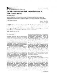
where pchild represents the offspring of the particle, p parent represents the parent of the particle, pc represents the crossover probability. pc ( pc ∈ [0,1] ) is a random number. Based on the trial and error, 0.2 was found to be a suitable value for pc . The two parents are combined to produce two new offspring. If the fitness of offspring is more than the fitness of parents, the offspring will be selected to replace the parents; otherwise, the offspring are discarded. 4.4. The Proposed Algorithm Flow The flow of the proposed algorithm is shown in Figure 1. In this flow, the parameters are set in step (1), and the particles are initialized in step (2). Its position is decoded in step (3), its corresponding fitness value is evaluated in step (4), its cognitive and social information is updated in step (5), and then moved by step (6). Step (7) is the controlling step for repeating or stopping the iteration. Step (8) generates a new set of the population. Note that the improvements of this flow from the original PSO take place in step (3), which uses the real encoding method to decode the route in addition to step (6), which introduces a linear decreasing function of the number of iterations, and step (8), which is combined with the crossover operator of genetic algorithm. The proposed algorithm steps are given as follows:

Sensors 2015, 15

21041

Figure 1. The flow of the proposed algorithm.

(1) Parameters setting. Define the parameters: acceleration coefficients k1 and k 2 , the maximum number of iterations η max , the initial value of inertia weight ω0 , the final value of inertia weight ωe , a random number pc , the number of the particles P , the maximum velocities of the particles vmax . (2) Population initiation. Initialize P particles as a population, generate the pth particle with 0 = x 0 pn . Set iteration η = 0 . random position x0 pn , velocity v0 pn , and personal best pbest pn (3) Particle encoding. According to the particle encoding rules, for i = 1,2,, p , decode xt pn to a set of route Rt pn . (4) Fitness evaluation. According to Equation (1), compute z , and then evaluate f fitness through Equation (9). t t t t < pbest , update pbest = pbest . If and gbest . If pbest (5) pbest and gbest updating. Compute pbest pn pn pn pn t t gbest < gbest , update gbest = gbest . pn pn

(6) Particles updating. Update the velocity and the position of each pth particle according to Equation (10). (7) Termination judgment. If the stopping criterion is met, go to step (9). Otherwise, η = η +1 and go to step (8). The stopping criterion is that η ≥ η max or finding a better solution. A better solution means that the hierarchical cost objective value is better than that of the best solution found so far.

Sensors 2015, 15

21042

(8) Crossover operator. Generate random number pc . According to Equations (13)–(16), generate a new set of population. Then return to step (3). (9) Outputting the optimal solution. Decode g best as the best set of vehicle route R and output the optimal solution R . 5. Experimental Results

In order to evaluate the performance of the proposed algorithm, we implemented the algorithm in Visual C# under Microsoft Windows-XP on a PC with Intel P4 4 GHz CPU and 2 GB RAM. The VRPTW benchmark problems of Solomon, which have been the most commonly chosen to evaluate and compare all algorithms, are tested in this paper. 5.1. Solomon Benchmark Problems It is well known that Solomon Benchmark problems are the widely used standard test set for VRPTW. Solomon Benchmark derives from the website [64]. The Solomon test set consists of 56 problem instances for each dimension category problem, i.e., 25, 50 and 100 customers. Each of these instances comprises 100 customers. The location of the depot and the customers are given as integer values from the range 0,1,,100 in a Cartesian coordinate system. The distance between two customers is the simple Euclidean distance. It is assumed that the travel times are equal to the corresponding Euclidean distances between the customer locations. One unit of time is necessary to run one unit of distance by any vehicle. Different capacity constraints are considered for the vehicle in each class of instance, as well as the demands from the customers. The test problems are grouped into six problem types: R1, R2, RC1, RC2, C1, and C2, each containing 8 to 12 instances. In R1 and R2, the customer locations are generated randomly in a given area according to a uniform distribution. C1 and C2 have customers located in clusters. RC1 and RC2 contain a mix of randomly distributed and clustered customers. R1, C1 and RC1 have narrow time windows and the vehicles have only small capacities. Therefore, each vehicle serves only a few customers. In contrast, R2, C2 and RC2- have wider windows and the vehicles have higher capacities. Each vehicle supplies more customers and therefore, compared to the type 1 problems, fewer vehicles are needed. Because the Solomon’s test set represents relatively well different kinds of scenarios, it has often been chosen to evaluate many solution proposals in the literature. 5.2. Evaluation of the Results In order to compare the solutions, four evaluation indexes are presented: the total traveled distance, the average total traveled distance, the CPU runtime and the quality of the solutions. The total traveled distance and the average total traveled distance are the main criteria in the VRPTW and determines the algorithm merits. The CPU runtime describes the algorithm efficiency. The quality of the solutions is the comprehensive index, which denotes the percentage of deviation from the best-known solution. The formula for calculating the percentage of deviation is as follows:

zdev =

z − zbest ×100% zbest

(17)

Sensors 2015, 15

21043

where zdev is the percentage of deviation from the best-known solution, z is the cost of the current solution, zbest is the cost of the best-known solution. 5.3. Analysis of the Results Each of 56 Solomon Benchmark problems is performed by some of the best-reported methods for VRPTW, namely, the genetic algorithm, ant colony optimization [29], PSO [65] and the proposed algorithm. Each problem involves 100 customers, randomly distributed over a geographical area. For each problem, 10 replications of the algorithm are attempted. According to Equation (1), we have adopted a formulation in which the total traveled distance is the optimized objective. Results displayed in the following tables contain the total traveled distance and the number of vehicles used in order to facilitate the comparison of our results with those obtained by hierarchical approaches in which the total traveled distance is the primary objective and, for the same total traveled distance, the secondary objective is number of vehicles, and also with multi-objective formulations that simultaneously consider both objectives [66]. It compares the total traveled distance (TD), the average total traveled distance, the CPU runtime and the quality of the solutions for each of the problems. Both best and average results are presented. 5.3.1. The Total Traveled Distance The results of TD and the number of vehicles (NV) are shown in Table 2. The published best-known solutions are not obtained by one or a particular class of methods [15,67–71]. Results emphasized in bold in Table 2 represent the new best solutions reached by the proposed algorithm: 1 out of 56 (1.79%). Results emphasized in bold and italic in Table 2 represent the previously best-known solutions that cannot be reached by this algorithm. The results show that many previously best-known solutions from the proposed algorithm have been reached: 31 out of 56 (55.4%). Globally, the TD average results are close to the optimal solutions known in the proposed algorithm. This comparison shows that the results from the proposed algorithm are competitive with other published results. In the genetic algorithm, 27 out of 56 (48.2%) have reached the previously best-known solutions. In PSO, 28 out of 56 (50%) have reached the previously best-known solutions. In ACO, 26 out of 56 (46.4%) have reached the previously best-known solutions. It can be seen that the proposed algorithm is better than the genetic algorithms, ACO and PSO. The efficiency is improved and the results are close to the best-known solutions. It is possible to see that the proposed algorithm continues to be very competitive in terms of total TD.

Sensors 2015, 15

21044 Table 2. The results of the total traveled distance for Solomon’s 100 customers set Problems.

No.

Problem

Best-Known Solution

PSO

Genetic Best

Average

Best

ACO Average

Best

The Proposed Algorithm Average

Best

Average

TD

NV

TD

NV

TD

NV

TD

NV

TD

NV

TD

NV

TD

NV

TD

NV

TD

NV

1

C101

828.94

10

828.94

10

856.26

10.20

828.94

10

842.60

10.10

828.94

10

842.60

10.10

828.94

10

842.60

10.10

2

C102

828.94

10

828.94

10

828.94

10.00

828.94

10

828.94

10.00

828.94

10

857.82

10.10

828.94

10

828.94

10.00

3

C103

828.06

10

828.06

10

859.88

10.00

828.06

10

828.06

10.00

828.06

10

828.06

10.00

828.06

10

828.06

10.00

4

C104

824.78

10

824.78

10

824.78

10.00

824.78

10

824.78

10.00

824.78

10

849.79

10.10

824.78

10

824.78

10.00

5

C105

828.94

10

828.94

10

854.25

10.20

828.94

10

866.91

10.30

828.94

10

904.88

10.60

828.94

10

841.60

10.10

6

C106

828.94

10

828.94

10

851.78

10.10

828.94

10

897.46

10.30

828.94

10

943.14

10.50

828.94

10

874.62

10.20

7

C107

828.94

10

828.94

10

856.47

10.20

828.94

10

842.70

10.10

828.94

10

870.23

10.30

828.94

10

842.70

10.10

8

C108

828.94

10

828.94

10

865.99

10.00

828.94

10

841.29

10.00

828.94

10

853.64

10.00

828.94

10

841.29

10.00

9

C109

828.94

10

828.94

10

910.27

10.30

828.94

10

856.05

10.10

828.94

10

883.16

10.20

828.94

10

828.94

10.00

10

C201

591.56

3

591.56

3

602.53

3.30

591.56

3

606.18

3.40

591.56

3

609.84

3.50

591.56

3

598.87

3.20

11

C202

591.56

3

591.56

3

656.01

3.20

591.56

3

623.78

3.10

591.56

3

623.78

3.10

591.56

3

591.56

3.00

12

C203

591.17

3

591.17

3

606.19

3.00

591.17

3

604.69

3.00

591.17

3

618.20

3.00

591.17

3

604.69

3.00

13

C204

590.60

3

590.60

3

704.28

3.30

590.60

3

666.39

3.20

590.60

3

742.17

3.40

590.60

3

628.49

3.10

14

C205

588.88

3

588.88

3

619.27

3.30

588.88

3

599.01

3.10

588.88

3

609.14

3.20

588.88

3

599.01

3.10

15

C206

588.49

3

588.49

3

620.28

3.20

588.49

3

604.38

3.10

588.49

3

636.17

3.30

588.49

3

588.49

3.00

16

C207

588.29

3

588.29

3

610.49

3.00

588.29

3

632.69

3.00

588.29

3

621.59

3.00

588.29

3

599.39

3.00

17

C208

588.32

3

588.32

3

622.73

3.00

588.32

3

599.79

3.00

588.32

3

611.26

3.00

588.32

3

599.79

3.00

18

R101

1483.57

16

1642.87

20

1645.83

19.50

1642.87

20

1645.33

19.50

1645.79

19

1647.29

19.00

1642.87

20

1645.83

19.50

19

R102

1355.93

14

1482.74

18

1483.75

17.70

1472.62

18

1477.95

17.80

1480.73

18

1482.21

17.80

1472.62

18

1477.14

17.80

20

R103

1133.35

12

1292.85

15

1248.88

14.40

1213.62

14

1239.30

14.40

1213.62

14

1247.22

14.30

1213.62

14

1239.01

13.80

21

R104

968.28

10

982.01

10

995.05

9.60

1007.24

9

1007.30

9.00

982.01

10

1000.11

9.40

982.01

10

992.52

9.70

22

R105

1262.53

12

1360.78

15

1366.87

14.80

1360.78

15

1374.14

14.70

1360.78

15

1369.99

15.30

1360.78

15

1366.42

15.00

23

R106

1201.78

12

1249.40

13

1251.48

12.20

1241.52

13

1249.39

12.40

1251.98

12

1252.00

12.00

1241.52

13

1247.29

12.60

24

R107

1051.92

11

1076.13

11

1094.18

10.70

1076.13

11

1094.19

10.50

1076.13

11

1096.08

10.70

1076.13

11

1088.49

10.70

25

R108

948.57

10

963.99

9

965.42

9.90

963.99

9

965.10

9.70

948.57

10

960.92

9.60

948.57

10

955.82

9.60

26

R109

1110.40

12

1151.84

13

1181.86

11.60

1151.84

13

1186.15

11.40

1151.84

13

1190.44

11.20

1151.84

13

1164.71

12.40

Sensors 2015, 15

21045 Table 2. Cont.

No.

Problem

27 28 29 30 31 32 33 34 35 36 37 38 39 40 41 42 43 44 45 46 47 48 49 50 51 52 53 54 55 56

R110 R111 R112 R201 R202 R203 R204 R205 R206 R207 R208 R209 R210 R211 RC101 RC102 RC103 RC104 RC105 RC106 RC107 RC108 RC201 RC202 RC203 RC204 RC205 RC206 RC207 RC208

Best-Known Solution TD 1080.36 987.80 953.63 1148.48 1049.74 900.08 772.33 959.74 898.91 814.78 715.37 879.53 932.89 761.10 1481.27 1395.25 1221.53 1135.48 1354.20 1226.62 1150.99 1076.81 1134.91 1113.53 945.96 796.11 1168.22 1059.89 976.40 785.93

NV 11 10 10 9 7 5 4 4 5 3 3 6 7 4 13 13 10 10 12 11 10 10 6 8 5 4 8 7 7 4

PSO

Genetic Best TD 1080.36 1053.50 982.14 1148.48 1049.74 900.08 807.38 970.89 898.91 814.78 725.75 879.53 954.12 885.71 1660.10 1466.84 1261.67 1135.48 1518.60 1377.35 1230.48 1117.53 1406.91 1365.57 945.96 798.41 1270.69 1059.89 999.26 816.10

Average NV 11 12 9 9 7 5 4 6 5 3 2 6 3 2 16 14 11 10 16 13 11 11 4 4 5 3 7 7 6 5

TD 1112.79 1086.43 995.33 1208.94 1086.62 930.23 828.06 982.66 906.06 844.73 726.61 892.08 955.06 892.31 1689.57 1493.53 1263.56 1135.50 1601.17 1396.59 1254.98 1135.32 1391.43 1250.18 1034.30 798.69 1276.08 1105.75 1060.37 824.93

NV 10.30 10.80 10.80 7.70 5.70 4.60 2.40 4.50 3.40 3.40 2.00 5.40 6.60 2.30 14.40 13.50 11.00 10.00 15.40 11.80 12.60 10.30 7.20 3.60 3.40 3.20 6.40 5.80 3.60 3.60

Best TD 1080.36 1053.50 953.63 1179.79 1049.74 932.76 772.33 970.89 906.14 814.78 725.42 879.53 954.12 885.71 1623.58 1482.91 1262.02 1135.48 1518.60 1384.92 1212.83 1117.53 1406.91 1113.53 945.96 798.41 1168.22 1084.30 976.40 816.10

ACO Average

NV 11 12 10 9 7 7 4 6 3 3 4 6 3 2 15 14 11 10 16 12 12 11 4 8 5 3 8 8 7 5

TD 1105.14 1083.13 965.03 1231.20 1100.68 939.72 817.42 980.30 910.24 868.25 725.77 891.00 954.64 889.53 1658.18 1497.28 1262.29 1135.50 1593.35 1417.25 1240.50 1127.41 1406.91 1162.75 1032.14 799.18 1282.01 1139.24 1011.75 822.41

NV 10.50 11.60 10.00 5.50 5.00 3.80 2.80 4.80 3.00 2.60 3.20 5.40 5.00 4.40 15.10 13.60 11.00 10.00 14.80 11.20 12.30 10.90 4.00 7.60 3.40 3.60 4.70 4.00 5.70 4.00

Best TD 1080.36 1088.48 953.63 1148.48 1079.36 939.54 772.33 970.89 906.14 814.78 725.75 879.53 939.34 888.73 1639.97 1477.54 1262.02 1135.48 1629.44 1377.35 1230.48 1117.53 1286.83 1113.53 1049.62 798.46 1168.22 1059.89 1053.58 806.87

The Proposed Algorithm Average

NV 11 12 10 9 6 3 4 6 3 3 2 6 3 5 16 13 11 10 13 13 11 11 9 8 3 3 8 7 6 5

TD 1107.72 1095.07 987.40 1212.51 1142.69 941.70 823.17 989.71 912.29 876.51 726.71 903.21 952.94 867.07 1687.56 1539.85 1264.17 1135.51 1633.29 1416.49 1258.04 1128.55 1397.23 1204.86 1052.87 799.43 1263.14 1135.44 1064.28 819.64

NV 10.50 10.40 10.60 7.30 4.10 3.00 2.80 3.60 3.00 2.60 2.00 4.20 4.78 2.90 14.40 12.30 11.00 10.00 13.00 11.30 12.80 10.80 6.00 6.30 3.00 3.80 6.80 4.00 3.90 4.00

Best TD 1080.36 1053.50 960.68 1148.48 1049.74 900.08 772.33 970.89 898.91 814.78 723.61 879.53 932.89 808.56 1623.58 1466.84 1261.67 1135.48 1618.55 1377.35 1212.83 1117.53 1387.55 1148.84 945.96 798.41 1161.81 1059.89 976.40 795.39

Average NV 11 12 10 9 7 5 4 6 5 3 3 6 7 4 15 14 11 10 16 13 12 11 8 9 5 3 7 7 7 5

TD 1098.14 1069.14 968.58 1178.39 1081.57 922.71 801.47 977.95 903.89 836.67 725.50 891.82 937.89 824.99 1645.18 1487.10 1262.04 1135.49 1621.16 1392.80 1226.01 1126.40 1391.43 1173.34 990.67 798.67 1187.56 1092.22 995.65 807.27

NV 10.70 11.60 9.90 8.40 5.70 4.60 3.40 5.10 4.00 3.00 2.50 5.10 6.20 3.90 15.10 13.50 11.00 10.00 15.40 12.30 12.00 10.70 7.20 7.90 4.20 3.20 6.90 6.00 6.40 4.78

Sensors 2015, 15

21046

5.3.2. The Average Total Traveled Distance The results of the average total traveled distance are shown in Table 3. Each entry refers to the best performance obtained with a specific technique over a particular data set. Rows C1, C2, R1, R2, RC1 and RC2 present the average number of vehicles and average total distance with respect to the six problem groups. The last row refers to the cumulative number of routes and traveled distance over all problem instances. The first column describes the various data sets and corresponding measures of performance defined by the average number of routes (or vehicles), and the total traveled distance. The following columns refer to particular problem-solving methods. The performance of the proposed algorithm is depicted in the last column. The results indicate that the proposed algorithm can match the best-known solutions, and it performs better than other algorithms. In addition, the proposed algorithm is the only method that found the minimum number of tours and the comparable traveled distance consistently for all problem data sets. Table 3. The results of the average total traveled distance. Problem

C1-type

C2-type

R1-type

R2-type

RC1-type

RC2-type

All

Best-Known Solution

Genetic Best

PSO

Average

Best

ACO

Average

Best

The Proposed Algorithm

Average

Best

Average

NV

10.00

10.00

10.11

10.00

10.10

10.00

10.21

10.00

10.06

TD

828.38

828.38

856.51

828.38

847.64

828.38

870.37

828.38

839.28

NV

3.00

3.00

3.16

3.00

3.11

3.00

3.19

3.00

3.05

TD

589.86

589.86

630.22

589.86

617.11

589.86

634.02

589.86

601.29

NV

11.67

13.00

12.69

12.92

12.63

12.92

12.57

13.08

12.78

TD

1128.18

1193.22

1202.32

1184.84

1199.35

1186.16

1203.04

1182.04

1192.76

NV

5.18

4.73

4.36

4.91

4.14

4.55

3.66

5.36

4.72

TD

893.90

912.31

932.12

915.56

937.16

914.99

940.77

899.98

916.62

NV

11.13

12.75

12.38

12.63

12.36

12.25

11.95

12.75

12.50

TD

1255.27

1346.01

1371.28

1342.23

1366.47

1358.73

1382.93

1351.73

1362.02

NV

6.13

5.13

4.60

6.00

4.63

6.13

4.73

6.38

5.82

TD

997.62

1082.85

1092.72

1038.73

1082.05

1042.13

1092.11

1034.28

1054.60

NV

449

465

452.40

472

448.70

466

441.88

483

466.68

TD

53,568.46

55,959.11

57,143.53

55,511.30

56,854.75

55,679.89

57,490.75

55,346.67

56,092.75

5.3.3. The Average Central Processing Unit (CPU) Runtime The results of the average CPU runtime are listed in Table 4. Rows C1, C2, R1, R2, RC1 and RC2- present the average CPU runtime with respect to the six problem groups. From Table 4, for the same instance, ACO is almost the most time consuming; the genetic algorithm takes second place; the PSO takes third place; and the proposed algorithm is last. The result shows that the proposed algorithm is highly efficient and suitable to be used in real-life problems to generate good solutions for further improvement. The average CPU runtime required to solve each type of problem set is between 62 and 149 milliseconds by the proposed algorithm, which is much faster than other algorithms. It can be seen that the proposed algorithm is very effective. This happened because crossover in GA is done between random chromosomes, whereas in the proposed algorithm, crossover is done between a particle’s

Sensors 2015, 15

21047

chromosome and best chromosome. Therefore, the proposed algorithm does not only give a better result, but it also reaches convergence results faster than other methods. Table 4. The results of the average CPU runtime. Problem Genetic PSO ACO The Proposed Algorithm C1e 98 85 111 62 C2 312 231 338 135 R1 112 81 124 60 R2 309 273 553 182 RC1 79 80 82 58 RC2 297 257 333 149

5.3.4. The Quality of the Solutions According to Equation (17), the quality of the solutions is shown in Table 5. Here z is the average total traveled distance. Rows C1, C2, R1, R2, RC1 and RC2 present the average zdev with respect to the six problem groups. The last row refers to the cumulative zdev over all problem instances. It can be seen that, with the proposed method, the quality of the results is between 1.32% and 8.17% with average quality equal to 4.07%; in the ACO, the quality of the solutions is between 5.07% and 9.75% with average quality equal to 6.95%; in PSO, the quality of the solutions is between 2.32% and 8.53% with average quality equal to 5.63%; in the genetic algorithm, the quality of the solutions is between 3.39% and 8.96% with average quality equal to 6.29%. The improvement in the quality of the solutions was achieved with the addition of the crossover operator of genetic algorithm. The reason is that, now, the particles moved in a more fast and efficient way to their local optimum or to the global optimum solution (to the best particle in the swarm). It is proved that the addition of the evolution of the population phase before the individuals used in the next generation improves the results of the algorithm, especially in the large-scale vehicle routing instances which are more difficult and time consuming. Table 5. The result of zdev . Problem Genetic PSO ACO The Proposed Algorithm C1-type 3.39% 2.32% 5.07% 1.32% C2-type 6.84% 4.62% 7.48% 1.94% R1-type 6.28% 5.98% 6.33% 5.36% R2-type 4.44% 4.93% 5.29% 2.62% RC1-type 8.89% 8.53% 9.75% 8.17% RC2-type 8.96% 7.92% 8.95% 5.30% All 6.29% 5.63% 6.95% 4.07%

From the results shown in Tables 2–5, it is observed that the proposed algorithm is fast and produces good solutions, which are only slightly less accurate than the best-known results. This comparison also shows that the results from the proposed algorithm are competitive with other published results. The experimental results reveal that the proposed algorithm is highly capable at minimizing the total travel distance. In particular, it is obvious that the proposed algorithm has great advantages for the solved problem size over the genetic algorithm, PSO and ACO. The reason is that,

Sensors 2015, 15

21048

now, the particles moved in a more fast and efficient way to their local optimum or to the global optimum solution (to the best particle in the swarm). After each environment change (peak movement), the particles are placed on a point far from the optimum through the inertia weight function. The particles take few iterations to reach this point. At the same time, the particle’s coding can be ensured that a particle is always able to generate a new feasible solution. 6. Conclusions

This paper proposes a genetic and PSO algorithm for VRPTW. Moreover, this algorithm was applied to the Solomon Benchmark problems and produced satisfactory results. Compared to other approaches, experimental results indicate that the proposed algorithm is fast and possesses a relatively accurate results. The proposed algorithm has proved to be an effective and competitive algorithm for the optimization problems due to its easy implementation, inexpensive computation and low memory requirements. Three major contributions are as follows: (1) The real encoding method avoids the complex encoding and decoding computation burden. (2) A linear decreasing function of the number of iterations in PSO have a flexible and well-balanced mechanism to enhance and adapt to the global and local exploration abilities, which can help find the optimal solution with the least number of iterations. (3) The crossover operator of the genetic algorithm is introduced to generate a new population guaranteeing that the offspring inherits good qualities from this parent. The crossover operator avoids premature convergence and local minimum value and increases the diversity of particles. Although the combination of the genetic algorithm and PSO for VRPTW obtains satisfactory achievements, there is still some room for improvement, such as how to effectively construct the initial solution and how to precisely judge the local optimal solution. Further research applying the proposed algorithm to other VRPTW variants will be carried out in our future work. Acknowledgements

This research was funded by National High Technology Research and Development Program of China (863 Program) under grant No. 2013AA122003 and No. 2012AA12A402, National Science & Technology Pillar Program under grant No. 2012BAB16B01, National Natural Science Foundation of P.R. China under grant No. 40901195, Special Fund for Quality Supervision, Inspection and Quarantine Research in the Public Interest under grant No. 201410308, and the Basic Research Fund of CASM. Author Contributions

Shenghua Xu and Jiping Liu conceived of and designed the study. Shenghua Xu and Liang Wang analyzed the data and performed the experiments. Shenghua Xu, Fuhao Zhang and Lijian Sun wrote and revised the paper extensively. All of the authors have read and approved the final manuscript.

Sensors 2015, 15

21049

Conflicts of Interest

The authors declare no conflict of interest. References

1. 2. 3. 4. 5. 6. 7. 8. 9. 10.

11.

12. 13.

14. 15. 16.

Dantzig, G.; Ramser, J. The truck dispatching problem. Manag. Sci. 1959, 6, 80–91. Hu, W.; Liang, H.; Peng, C.; Du, B.; Hu, Q. A hybrid chaos-particle swarm optimization algorithm for the vehicle routing problem with time window. Entropy 2013, 15, 1247–1270. Bräysy, O. A reactive variable neighborhood search for the vehicle-routing problem with time windows. INFORMS J. Comput. 2003, 15, 347–368. Belenguer, J.-M.; Benavent, E.; Prins, C.; Prodhon, C.; Calvo, R.W. A branch-and-cut method for the capacitated location-routing problem. Comput. Oper. Res. 2011, 38, 931–941. Jepsen, M.; Spoorendonk, S.; Ropke, S. A branch-and-cut algorithm for the symmetric two-echelon capacitated vehicle routing problem. Transp. Sci. 2013, 47, 23–37. Niebles, J.; Wang, H.; Fei-Fei, L. Unsupervised learning of human action categories using spatial-temporal words. Int. J. Comput. Vis. 2008, 79, 299–318. Vidal, T.; Crainic, T.G.; Gendreau, M.; Prins, C. Heuristics for multi-attribute vehicle routing problems: A survey and synthesis. Eur. J. Oper. Res. 2013, 231, 1–21. Berbeglia, G.; Cordeau, J.-F.; Laporte, G. A hybrid tabu search and constraint programming algorithm for the dynamic dial-a-ride problem. INFORMS J. Comput. 2012, 24, 343–355. Pillac, V.; Gendreau, M.; Guéret, C.; Medaglia, A.L. A review of dynamic vehicle routing problems. Eur. J. Oper. Res. 2013, 225, 1–11. Andres Figliozzi, M. The time dependent vehicle routing problem with time windows: Benchmark problems, an efficient solution algorithm, and solution characteristics. Transp. Res. Part E Logist. Transp. Rev. 2012, 48, 616–636. Çetinkaya, C.; Karaoglan, I.; Gökçen, H. Two-stage vehicle routing problem with arc time windows: A mixed integer programming formulation and a heuristic approach. Eur. J. Oper. Res. 2013, 230, 539–550. Yu, B.; Yang, Z.; Yao, B. A hybrid algorithm for vehicle routing problem with time windows. Expert Syst. Appl. 2011, 38, 435–441. Anbuudayasankar, S.; Ganesh, K.; Koh, S.L.; Ducq, Y. Modified savings heuristics and genetic algorithm for bi-objective vehicle routing problem with forced backhauls. Expert Syst. Appl. 2012, 39, 2296–2305. Repoussis, P.P.; Tarantilis, C.D.; Ioannou, G. Arc-guided evolutionary algorithm for the vehicle routing problem with time windows. IEEE Trans. Evol. Comput. 2009, 13, 624–647. Garcia-Najera, A.; Bullinaria, J.A. An improved multi-objective evolutionary algorithm for the vehicle routing problem with time windows. Comput. Oper. Res. 2011, 38, 287–300. Prescott-Gagnon, E.; Desaulniers, G.; Rousseau, L.M. A branch-and-price-based large neighborhood search algorithm for the vehicle routing problem with time windows. Networks 2009, 54, 190–204.

Sensors 2015, 15

21050

17. Azi, N.; Gendreau, M.; Potvin, J.Y. An exact algorithm for a vehicle routing problem with time windows and multiple use of vehicles. Eur. J. Oper. Res. 2010, 202, 756–763. 18. Cordeau, J.F.; Maischberger, M. A parallel iterated tabu search heuristic for vehicle routing problems. Comput. Oper. Res. 2012, 39, 2033–2050. 19. Brandão, J. A tabu search algorithm for the heterogeneous fixed fleet vehicle routing problem. Comput. Oper. Res. 2011, 38, 140–151. 20. Escobar, J.W.; Linfati, R.; Toth, P.; Baldoquin, M.G. A hybrid granular tabu search algorithm for the multi-depot vehicle routing problem. J. Heuristics 2014, 20, 483–509. 21. Archetti, C.; Bouchard, M.; Desaulniers, G. Enhanced branch and price and cut for vehicle routing with split deliveries and time windows. Transp. Sci. 2011, 45, 285–298. 22. Hashimoto, H.; Yagiura, M.; Ibaraki, T. An iterated local search algorithm for the time-dependent vehicle routing problem with time windows. Discret. Opt. 2008, 5, 434–456. 23. Michallet, J.; Prins, C.; Amodeo, L.; Yalaoui, F.; Vitry, G. Multi-start iterated local search for the periodic vehicle routing problem with time windows and time spread constraints on services. Comput. Oper. Res. 2014, 41, 196–207. 24. Li, X.; Tian, P.; Leung, S.C.H. Vehicle routing problems with time windows and stochastic travel and service times: Models and algorithm. Int. J. Prod. Econ. 2010, 125, 137–145. 25. Yu, B.; Yang, Z.Z. An ant colony optimization model: The period vehicle routing problem with time windows. Transp. Res. Part E Logist. Transp. Rev. 2011, 47, 166–181. 26. Dhahri, A.; Zidi, K.; Ghedira, K. A Variable Neighborhood Search for the Vehicle Routing Problem with Time Windows and Preventive Maintenance Activities. Electron. Notes Discret. Math. 2015, 47, 229–236. 27. Khouadjia, M.R.; Sarasola, B.; Alba, E.; Jourdan, L.; Talbi, E.-G. A comparative study between dynamic adapted PSO and VNS for the vehicle routing problem with dynamic requests. Appl. Soft Comput. 2012, 12, 1426–1439. 28. Brandão de Oliveira, H.C.; Vasconcelos, G.C. A hybrid search method for the vehicle routing problem with time windows. Ann. Oper. Res. 2010, 180, 125–144. 29. Balseiro, S.; Loiseau, I.; Ramonet, J. An Ant Colony algorithm hybridized with insertion heuristics for the Time Dependent Vehicle Routing Problem with Time Windows. Comput. Oper. Res. 2011, 38, 954–966. 30. Szeto, W.; Wu, Y.; Ho, S.C. An artificial bee colony algorithm for the capacitated vehicle routing problem. Eur. J. Oper. Res. 2011, 215, 126–135. 31. Mahdavi, V.; Sadeghi, S.A.; Fathi, S. A mathematical Model and Solving Method for Multi-Depot and Multi-level Vehicle Routing Problem with Fuzzy Time Windows. Adv. Intel. Transp. Syst. 2012, 1, 19–24. 32. El-Sherbeny, N.A. Vehicle routing with time windows: An overview of exact, heuristic and metaheuristic methods. J. King Saud Univ. Sci. 2010, 22, 123–131. 33. Bhagade, A.S.; Puranik, P.V. Artificial bee colony (ABC) algorithm for vehicle routing optimization problem. Int. J. Soft Comput. Eng. 2012, 2, 329–333. 34. Ai, T.; Kachitvichyanukul, V. A particle swarm optimization for the vehicle routing problem with simultaneous pickup and delivery. Comput. Oper. Res. 2009, 36, 1693–1702.

Sensors 2015, 15

21051

35. Kok, A.L.; Meyer, C.M.; Kopfer, H.; Schutten, J.M.J. A dynamic programming heuristic for the vehicle routing problem with time windows and European Community social legislation. Transp. Sci. 2010, 44, 442–454. 36. Erdoğan, S.; Miller-Hooks, E. A green vehicle routing problem. Transp. Res. Part E Logist. Transp. Rev. 2012, 48, 100–114. 37. Küçükoğlu, İ.; Öztürk, N. An advanced hybrid meta-heuristic algorithm for the vehicle routing problem with backhauls and time windows. Comput. Ind. Eng. 2015, 86, 60–68. 38. Marinakis, Y.; Marinaki, M. A hybrid genetic–Particle Swarm Optimization Algorithm for the vehicle routing problem. Expert Syst. Appl. 2010, 37, 1446–1455. 39. Nagata, Y.; Bräysy, O.; Dullaert, W. A penalty-based edge assembly memetic algorithm for the vehicle routing problem with time windows. Comput. Oper. Res. 2010, 37, 724–737. 40. Dey, S.; Bhattacharyya, S.; Maulik, U. Quantum inspired genetic algorithm and particle swarm optimization using chaotic map model based interference for gray level image thresholding. Swarm Evol. Comput. 2014, 15, 38–57. 41. Valdez, F.; Melin, P.; Castillo, O. Modular neural networks architecture optimization with a new nature inspired method using a fuzzy combination of particle swarm optimization and genetic algorithms. Inf. Sci. 2014, 270, 143–153. 42. Ru, N.; Yue, J. A GA and particle swarm optimization based hybrid algorithm. In Proceedings of the IEEE Congress on Evolutionary Computation, Hong Kong, China, 1–6 June 2008; pp. 1047–1050. 43. Hao, Z.-F.; Wang, Z.-G.; Huang, H. A particle swarm optimization algorithm with crossover operator. In Proceedings of the 2007 IEEE International Conference on Machine Learning and Cybernetics, Hong Kong, China, 19–22 August 2007; pp. 1036–1040. 44. Masrom, S.; Abidin, S.Z.; Omar, N.; Nasir, K.; Abd Rahman, A. Dynamic parameterization of the particle swarm optimization and genetic algorithm hybrids for vehicle routing problem with time window. Int. J. Hybrid Int. Syst. 2015, 12, 13–25. 45. Kuo, R.; Zulvia, F.E.; Suryadi, K. Hybrid particle swarm optimization with genetic algorithm for solving capacitated vehicle routing problem with fuzzy demand—A case study on garbage collection system. Appl. Math. Comput. 2012, 219, 2574–2588. 46. Dhahri, A.; Zidi, K.; Ghedira, K. Variable Neighborhood Search based Set Covering ILP Model for the Vehicle Routing Problem with Time Windows. Proc. Comput. Sci. 2014, 29, 844–854. 47. Sha, D.; Hsu, C. A new particle swarm optimization for the open shop scheduling problem. Comput. Oper. Res. 2008, 35, 3243–3261. 48. Lian, Z.; Gu, X.; Jiao, B. A novel particle swarm optimization algorithm for permutation flow-shop scheduling to minimize makespan. Chaos Solitons Fract. 2008, 35, 851–861. 49. Jarboui, B.; Damak, N.; Siarry, P.; Rebai, A. A combinatorial particle swarm optimization for solving multi-mode resource-constrained project scheduling problems. Appl. Math. Comput. 2008, 195, 299–308. 50. Shi, X.; Liang, Y.; Lee, H.; Lu, C.; Wang, Q. Particle swarm optimization-based algorithms for TSP and generalized TSP. Inf. Process. Lett. 2007, 103, 169–176. 51. Jarboui, B.; Cheikh, M.; Siarry, P.; Rebai, A. Combinatorial particle swarm optimization (CPSO) for partitional clustering problem. Appl. Math. Comput. 2007, 192, 337–345.

Sensors 2015, 15

21052

52. Pan, Q.; Fatih Tasgetiren, M.; Liang, Y. A discrete particle swarm optimization algorithm for the no-wait flowshop scheduling problem. Comput. Oper. Res. 2008, 35, 2807–2839. 53. Yin, P.-Y.; Yu, S.-S.; Wang, P.-P.; Wang, Y.-T. A hybrid particle swarm optimization algorithm for optimal task assignment in distributed systems. Comput. Stand. Int. 2006, 28, 441–450. 54. Bohre, A.K.; Agnihotri, G.; Dubey, M.; Singh, J. A Novel Method to Find Optimal Solution Based on Modified Butterfly Particle Swarm Optimization. Int. J. Soft Comput. Math. Control 2014, 3, 1–14. 55. Ping, H.J.; Lian, L.Y.; Xing, H.; Hua, W.J. A Novel Hybrid Algorithm with Marriage of Particle Swarm Optimization and Homotopy Optimization for Tunnel Parameter Inversion. Appl. Mech. Mater. 2012, 229–231, 2033–2037. 56. Shi, Y.; Eberhart, R. A modified particle swarm optimizer. In Proceedings of the IEEE International Conference on Evolutionary Computation, Anchorage, AK, USA, 4–9 May 1998; pp. 69–73. 57. Jiao, B.; Lian, Z.; Gu, X. A dynamic inertia weight particle swarm optimization algorithm. Chaos Solitons Fract. 2008, 37, 698–705. 58. Liu, X.; Wang, Q.; Liu, H.; Li, L. Particle swarm optimization with dynamic inertia weight and mutation. In Porceedings of the 3rd IEEE International Conference on Genetic and Evolutionary Computing, Guilin, China, 14–17 October 2009; pp. 620–623. 59. Tao, Z.; Cai, J. A new chaotic PSO with dynamic inertia weight for economic dispatch problem. In Proceedings of the IEEE International Conference on Sustainable Power Generation and Supply, Nanjing, China, 6–7 April 2009; pp. 1–6. 60. Tripathi, P.K.; Bandyopadhyay, S.; Pal, S.K. Multi-objective particle swarm optimization with time variant inertia and acceleration coefficients. Inf. Sci. 2007, 177, 5033–5049. 61. Nickabadi, A.; Ebadzadeh, M.M.; Safabakhsh, R. A novel particle swarm optimization algorithm with adaptive inertia weight. Appl. Soft Comput. 2011, 11, 3658–3670. 62. Shen, X.; Chi, Z.; Yang, J.; Chen, C. Particle swarm optimization with dynamic adaptive inertia weight. In Proceedings of the IEEE International Conference on Challenges in Environmental Science and Computer Engineering, Wuhan, China, 6–9 March 2010; pp. 287–290. 63. Zhang, L.; Tang, Y.; Hua, C.; Guan, X. A new particle swarm optimization algorithm with adaptive inertia weight based on Bayesian techniques. Appl. Soft Comput. 2015, 28, 138–149. 64. VRPTW Benchmark Problems. Available online: http://web.cba.neu.edu/~msolomon/ problems.htm (accessed on 26 August 2015). 65. Ai, T.J.; Kachitvichyanukul, V. A particle swarm optimisation for vehicle routing problem with time windows. Int. J. Oper. Res. 2009, 6, 519–537. 66. Baños, R.; Ortega, J.; Gil, C.; Márquez, A.L.; de Toro, F. A hybrid meta-heuristic for multi-objective vehicle routing problems with time windows. Comput. Ind. Eng. 2013, 65, 286–296. 67. Barbucha, D. A cooperative population learning algorithm for vehicle routing problem with time windows. Neurocomputing 2014, 146, 210–229. 68. Ghannadpour, S.F.; Noori, S.; Tavakkoli-Moghaddam, R.; Ghoseiri, K. A multi-objective dynamic vehicle routing problem with fuzzy time windows: Model, solution and application. Appl. Soft Comput. 2014, 14, 504–527.

Sensors 2015, 15

21053

69. Taş, D.; Jabali, O.; van Woensel, T. A vehicle routing problem with flexible time windows. Comput. Oper. Res. 2014, 52, 39–54. 70. Barb, A.S.; Shyu, C.R. A study of factors that influence the accuracy of content-based geospatial ranking systems. Int. J. Image Data Fusion 2012, 3, 257–268. 71. Alvarenga, G.B.; Mateus, G.R.; de Tomi, G. A genetic and set partitioning two-phase approach for the vehicle routing problem with time windows. Comput. Oper. Res. 2007, 34, 1561–1584. © 2015 by the authors; licensee MDPI, Basel, Switzerland. This article is an open access article distributed under the terms and conditions of the Creative Commons Attribution license (http://creativecommons.org/licenses/by/4.0/).