ROGER PENROSE. I want to describe an idea which is related to other things
that were suggested in the colloquium, though my approach will be quite different
.
Whereas such combinatorial problems are extremely difficult to solve ... get functional, lead examples being detection of multi- ...... agement, 5, 81â102 (1978). 9.
Aug 8, 2012 - spaces (see [3]), but also to show that an Orlicz space with a ... with x ∈ Rn, y ∈ Rn×n, and express their order in terms of .... x = xJ + xI ∈ 3B. D ...
G. Clift, 'Crystal bases and Young tableaux', Journal of Algebra 202 N1(1998) ... S. Montgomery, Hopf Algebras and Their Actions on Rings (CBMS 82, AMS,.
arXiv:math/0002149v1 [math.QA] 17 Feb 2000 ... In the present paper we propose a combinatorial solution of this problem by means of the quantum (Lie) .... ential operators. Immediately afterwards a number of interesting questions appears. ...... Jour
Feb 1, 2008 - To appear in Advances in Chemical Engineering. 1 ...... of catalysis, sensors, coatings, microelectronics, biotechnology, and .... Riddle, D. S., Santiago, J. V., Brayhall, S. T., Doshi, N., Grantcharova, V. P., Yi, Q., and Baker, D.,.
Jan 18, 2001 - One model that has found a large number of successful applications is the threshold autoregressive model (TAR). The TAR model is a ...
group Î generated by the reflections of X in the sides of â is an n-simplex discrete re- ... n-simplex (spherical, euclidean and hyperbolic) reflection groups is ...
May 25, 2015 - of Reidemeister moves that untangles an unknot, has been ... tricolorability is invariant with respect to Reidemeister moves, and so it is a.
Feb 6, 2015 - Side Groups that Stabilize DNA-Templated. Supramolecular Self-Assemblies. Delphine Paolantoni, Sonia Cantel, Pascal Dumy and Sébastien ...
Background. A fragmentation of genomic DNA by restriction digestion is a popular step in many applications. Usually attention is paid to the expected average ...
Otherwise the swap is not made and the process restarts with another household .... The counts of males and females in categories 'Husband (wife) in a regis-.
Mathematical models in the biological and ecological sciences frequently use ....
can be found in Rosen's combinatorics handbook [8] as well as most other ...
actions are the choices of the next city to visit, and the action-values indicate the desirability of the city to visit next. ..... finding a permutation Ï minimizing: â.
samples only a tiny fraction of the search space, these re- sults are quite ... of organic evolution as an attempt to solve hard optimiza- tion and adaptation tasks ...
Aug 4, 2010 - topological considerations 6,7,9 to the study of the influ- ence that ..... involves a systematic search f
Aug 24, 2018 - reliability analysis of 6T SRAM and discover the variance among different ... technique to improve energy efficiency by lowering the supply voltage to ... To reduce the overall performance overhead of our proposed opportunistic supply
Aug 4, 2010 - Commu- nities are groups of nodes with a high level of internal and ... The last few years have witnessed
endgame problems with solution lengths ex- ceeding 60 moves. 1 Introduction. In two-player games with perfect information, minimax- based search methods ...
main ideas of our approach are best illustrated by the basic problem of continuously reconfiguring a simple planar polygon to any other planar configuration with.
Jul 19, 2014 - To fulfill this goal, a computer code was developed on the basis of zeroâone ... a reliable way of evaluating the particle size distribution (PSD).
requirements for an effective combinatorial testing tool, extending the previous ... testing with model checking (SMV) to provide automated specification based ... to be covered is motivated by a performance improvement it produces on the.
presented by F.T. Howard and Curtis Cooper in the August, 2011, issue of ... I would like to thank my advisor, Professor Arthur Benjamin, and my sec- ond reader ...
Mar 15, 2016 - Abstract: In this paper, simple models for the multiverse are analyzed. Each universe is viewed as a path in a graph, and by considering very ...
Article
A Combinatorial Approach to Time Asymmetry Martin Tamm Department of Mathematics, University of Stockholm, Stockholm 10691, Sweden; [email protected]; Tel.: +46-708775876 Academic Editor: Purushottam D. Gujrati Received: 30 November 2015 ; Accepted: 8 March 2016; Published: 15 March 2016
Abstract: In this paper, simple models for the multiverse are analyzed. Each universe is viewed as a path in a graph, and by considering very general statistical assumptions, essentially originating from Boltzmann, we can make the set of all such paths into a finite probability space. We can then also attempt to compute the probabilities for different kinds of behavior and in particular under certain conditions argue that an asymmetric behavior of the entropy should be much more probable than a symmetric one. This offers an explanation for the asymmetry of time as a broken symmetry in the multiverse. The focus here is on simple models which can be analyzed using methods from combinatorics. Although the computational difficulties rapidly become enormous when the size of the model grows, this still gives hints about how a full-scale model should behave. Keywords: multiverse, graph, time’s arrow, cosmology, entropy
1. Introduction The problem of Time’s Arrow, or "the riddle of time", consists in the observation that on the macroscopic level, time is asymmetric and directed (we can remember the past but not the future), whereas on the microscopic level, all the laws of nature which are supposed to be responsible for the macroscopic behavior, are essentially time-symmetric. So where does the asymmetry come from? A general reference for this discussion is Zeh [1]. For a philosophical discussion of some of the traps that physicists tend to fall into when investigating these matters, see Price [2]. Although there is still no consensus about what the answer to the riddle should be, a major step towards a solution was taken already in the 19th century. In fact, it took the genius of Ludwig Boltzmann [3] to realize that this has something to do with the fact that the universe during its development passes from less probable states to more probable ones, and that this is very closely related to the growth of the entropy as expressed by the second law of thermodynamics. However, Boltzmann’s idea can by itself never fully explain time asymmetry for the simple reason that it already has a direction of time built into it. This paper is part of an approach, based on reformulating Boltzmann’s idea in a time symmetric way. A clue to how this may be done is given by considering not just our own universe, but all possible universes. Although quantum mechanics is in principle deterministic, from the point of view of an observer there are always many possible different futures. For example, every quantum measurement where the outcome is stochastic can be viewed as a fork in the road, where different outcomes may rapidly diverge into different developments. And since the dynamic laws are essentially time-symmetric, it seems reasonable to argue that from a local point of view, given any state of a universe at any time, there should be many possible developments leading to higher entropy (and very few leading to lower entropy) in both directions of time. As we will see however, this point of view may be very well compatible with the idea that from a global point of view, in the set of all universes, a monotonic behavior of the entropy is far more probable than a non-monotonic one.
Symmetry 2016, 8, 11; doi:10.3390/sym8030011
www.mdpi.com/journal/symmetry
Symmetry 2016, 8, 11
2 of 10
This naturally leads us to consider models for the so called Time’s Arrow, where the asymmetry of time is viewed as a broken symmetry in the symmetric space of all possible universes; it may be that in 50% of all universes, the Arrow points in one direction, and in 50% of them it points in the other. Still, each observer (confined to just one universe) will observe a definite direction of time. In [4] and [5], the physical background for this approach is discussed in more detail, although the methods used there are heuristic. In this paper I instead concentrate on very simple models where it is possible to use exact combinatorial methods. However, the computational difficulties rapidly become enormous, and even small examples of such models can be a challenge for modern computer technology. Let me state explicitly that the purpose of this paper is not to present new deep mathematical results. Rather, it is the use of this kind of models in itself which is the issue. The calculations here should mainly be considered as comparatively simple examples of how this kind of models for the multiverse can be investigated. But in fact, analyzing such examples can give valuable hints to what should be expected from a full-scale model. It is my personal belief that the best way to make progress towards a solution of the riddle of time is to work in both directions; not only can investigations of small models illuminate our understanding of the realistic case, but in the same time our understanding and our ideas about the realistic case must be used to modify the models. In particular, I will argue that although the simplest kind of model in this paper may be sufficient to explain why a monotonic behavior of the entropy is much more probable than a behavior with low entropy at both ends, it may still be that we need more complicated models to understand the relation to other kinds of behavior, e.g., high entropy at both ends. Hence, the real purpose of this paper is rather to introduce a new way of approaching the question about the asymmetry of time. In the same time, this may also turn out to be a new area where abstract mathematics and numerical computations can interact in a interesting way. 2. Mathematical Preliminaries In this paper, the most essential tools come from graph theory. Since this is somewhat unusual for cosmology in general and for the question of time asymmetry in particular, I will here summarize the main facts that will be used. For a more complete treatment, see [6] and [7]. A graph G is determined by a set of V of nodes (or vertices) and a set E of edges, where each edge e = [v1 , v2 ] can be viewed as pair of nodes v1 , v2 ∈ V, in which case we say that v1 and v2 are connected by e. In an undirected graph, the roles of v1 and v2 are symmetric, but in this paper we will mainly consider directed graphs, which means that the first node is the starting-point and the second is the end-point of the edge. In this paper, the set V will always be finite. A (directed) path [v1 , v2 , . . . , vm ] from v1 to vm is a sequence of nodes with the property that for each j = 1, 2, . . . , m − 1, the pair v j , v j+1 belongs to the set of (directed) edges of the graph. It is a fundamental problem in graph theory to compute the number of paths starting at one given node and and ending up at another one. For a general graph, this problem may be very difficult in the sense that the number of computations to be carried out grows very rapidly with the size of the graph. However, for graphs with additional properties, the problem may simplify considerably. In particular, the special time-related structure of the graphs in this paper will imply that all paths joining two nodes will always have the same length (equal to the number of units of time separating the two nodes). In this situation, it very natural to make use of the following Definition 1. The adjacency matrix of the (directed) graph G with nodes v1 , v2 , . . . , vm is the m × m-matrix A = ( aij ), where aij = 1 if the pair vi , v j determines a (directed) edge in G and aij = 0 otherwise. The importance of this concept for the present paper lies in the following well-known
Symmetry 2016, 8, 11
3 of 10
Theorem 2. The element at position ij of the k:th power of the adjacency matrix, Ak , equals the number of paths of length k, starting at vi and ending at v j . Once formulated in the right way, the proof of the theorem is almost trivial. In fact, by the definition of matrix multiplication,
( Ak )ij =
m
m
∑ ∑
q1 =1 q2 =1
m
···
∑
q k −1 =1
aiq1 aq1 q2 · · · aqk−1 j ,
(1)
and aiq1 aq1 q2 · · · aqk−1 j = 1 if and only if [vi , vq1 , vq2 , . . . , vk−1 , j] is a (directed) path from vi to v j and 0 otherwise. Thus, each such path will contribute with exactly one to the sum. 3. To model the universe What is a good model for the universe? The answer to this question of course depends both on what properties we want to model and on the theoretical framework that we have chosen. If our starting point is quantum mechanics, it may be natural to describe the universe by a huge wave function, developing in time. If our starting point is instead general relativity, a more natural model would perhaps be a pseudo-Riemannian manifold with some distribution of mass-energy. One can wish for a more general model which can account for both quantum mechanical and relativistic phenomena, but we are not quite there yet; so far, different models can explain different aspects of the universe, but no single model can explain everything. In this paper, I will consider still another model for the universe, namely as a path in an enormous graph. Needless to say, this model is not intended to be a serious alternative for explaining all the properties that a quantum mechanical or a general relativistic model can explain. It is just an attempt to extract a sort of skeleton for the dynamics of our universe. Having said this, it may also be worthwhile to note that this skeleton represents a perspective on the idea of multiple histories or "the multiverse" which is somewhat different from the usual view. In fact, this multiverse makes sense both within classical and quantum physics, rather than just being a consequence of the laws of quantum mechanics. In the following, I will only be concerned with closed models for the universe. Also, I will study what could be called discrete universes or perhaps discrete approximations to universes. In particular, I will assume that there are only a finite number of moments of time between the Big Bang and a supposed Big Crunch, and for each such moment of time, there will be only a finite number of possible states. How these states should be understood, quantum mechanically, classically or in still some other way, is a complicated question which will not be discussed here. The reader is instead referred to [4] and [5]. In view of the enormous complexity of the universe, it is necessary to make drastic simplifications, and the main idea of the model in this paper is to suppress all dynamical properties except for entropy. According to Boltzmann, the total entropy of a certain macro-state at a certain time is given by S = k B log Ω, (2) or inversely Ω = WS,
with
W = e1/k B ,
(3)
where Ω denotes the number of corresponding micro-states, and k B is Boltzmann’s constant. Although this formula was derived under quite special circumstances, it is generally agreed to contain an almost universal truth about nature. In particular, I will in the following take for granted that the total number of possible states of a universe, with a given entropy S at a particular moment of time, is an exponential function of the total entropy as in Equation (3).
Symmetry 2016, 8, 11
4 of 10
If the total number of states is finite, then this assumption can of course only hold true as long as the entropy is not near to becoming maximal. However, in this paper I will assume that the life-span of the universe (i.e., the time interval between the Big Bang and the Big Crunch) is short in comparison with the time required for this to happen. In fact, according to [8] and [9], it would take a very long time for our universe to reach such a state. For a given state at a given moment of time t, the dynamical laws will only permit transitions to a very limited number of states at the previous and next moments of time. Needless to say, in reality there is no absolute distinction between possible and impossible transitions, but for the purpose of this paper, I will still make this simplifying assumption. Summarizing: Definition 3. A universe U is a chain of states (one state Ut for each moment of time t), with the property that the transition between adjacent states is always possible. Definition 4. The multiverse M is the set of all possible universes U in the sense of Definition 3. 4. How many universes of different types are there? It is now time to turn the ideas of the previous section into a combinatorial model where explicit computations can be made. To make things as simple as possible, let me choose a time-axis as follows Figure 1:
Figure 1. The time axis.
Here − T0 and T0 represent the Big Bang and the Big Crunch respectively, and the discrete moments of time correspond to the integers in the interval in between, which is symmetric about the origin. The first and last parts, [− T0 , − T1 ] and [ T1 , T0 ] can be said to represent the extreme phases near the end points, where the ordinary laws of physics may not apply. The interval in between, [− T1 , T1 ], could be called the normal phase, where the laws of physics behave essentially as we are used to. Of course, the distinction is not sharp, but may still make sense in a model like this. Let us start the investigation by considering this normal phase, and come back to the extreme phases in Section 5. For each moment of time in the interval [− T1 , T1 ], let us think of all the possible states of a universe as the nodes in a graph. If a transition between two states (at adjacent moments of time) is possible, then the corresponding nodes are joined by an edge, and a specific universe can thus be viewed as a path with one node for each moment of time in the corresponding graph. To specify the dynamics is in this context equivalent to defining the set of edges in the graph. In the present paper, this is done by assuming that for any state Σ with entropy S (except at the end points), there are exactly M edges connecting Σ to states at time t + 1 with entropy S + 1, and these will be chosen completely at random among such states. Similarly, there will be exactly the same number M of edges connecting Σ to states at time t − 1 with entropy S + 1. In the following, W in (3) will always be larger than M, and in cases of physical interest it should actually be much larger. In particular, this means that among all states with entropy S + 1 at a certain moment of time t, only a minor fraction can be reached from states with lower entropy at times t + 1 or t − 1. In other words, only comparatively few states Σ have edges connecting to states with lower entropy in any of the two directions of time. The assumption that S can only increase or decrease with one unit amount of entropy per unit of time is of course an extreme simplification. In a slightly more developed version of this model, this assumption should clearly be replaced by something more realistic.
Symmetry 2016, 8, 11
5 of 10
Remark 1. Summing up, let us note that the dynamical assumptions above are time-symmetric; the choices of the edges are to a certain extent at random, but if we consider the totality of all such graphs, this set will be preserved if we reverse the direction of the time-axis. In particular, when we consider mean values, these will be time-symmetric. Also, the dynamics reflects Boltzmann’s idea of the universe as developing from less probable states to more probable states in the sense that for any randomly chosen state there will always be several possible developments towards higher entropy but only a small chance that there will be a development towards lower entropy. It is essential to note that this is true in both directions of time. In Figure 2 is shown a schematic picture of the set of all possible states and three possible universes in the case of a (very) small graph with only 5 moments of time, and with W = 4. Note that according to the dynamical assumptions above, no universe starting with S = 0 at one end can ever attain a value of S larger than 4, hence the part of the graph shown is perfectly enough for comparing universes with low entropy at at least one end. To exploit this simple case further, let me show how to compute the number of paths of different types. For the rest of this section, let M = 2.
Figure 2. A schematic picture of three universes during the normal phase, as particular paths in the graph of all possible states, in a very small model with only five moments of time from − T1 = −2 to T1 = 2. The red path has a monotonic behavior of the entropy whereas the blue paths represent developments with low entropy at both ends.
It is trivial to compute the number of paths with monotonically increasing entropy. The assumption M = 2 implies that for each unit of time the number obviously doubles: According to the above construction, from the state with S = 0 at time − T1 , there are exactly two edges connecting to states with S = 1 at time − T1 + 1. From each of these two states, there will also be exactly two edges connecting to states with S = 2 at time − T1 + 2 which gives four paths so far. At the next step we get eight paths ending at states with S = 3 at time − T1 + 3 and so on. In the case − T1 = −2 and T1 = 2, we get 24 = 16 such paths, since there are only four unit intervals of time in between, and similarly for − T1 = −3 and T1 = 3, we get 26 = 64 paths since there are six unit intervals of time in between. It is much more work to compute the number of paths with low entropy at both ends; this number will in fact be a statistical variable which varies with the random dynamics, defined by the edges in the graph. Also, what will actually be computed is the estimated average number of such paths over a large number of different graphs. To do the computation, I will make use of the adjacency matrix of the graph (see Section 2). Note that the use of directed graphs here has nothing to do with introducing some kind of presupposed direction of time in the model. It is just a way of reducing the number of non-zero elements in the
Symmetry 2016, 8, 11
6 of 10
adjacency matrix. In fact, in the graphs of this paper, a directed path from t = − T1 to t = T1 is exactly the same thing as an ordinary path of length 2T1 from t = − T1 to t = T1 (if we forget about the directions). In view of the way the adjacency matrix will be set up below, all information about paths starting with S = 0 at − T1 will be contained in the first row of Am . Thus, all we need to do is to write down the matrix A and compute. This is not difficult in theory, but the size of A grows rapidly with the number of time intervals and with W. To compute all possible paths starting with S = 0 at time − T1 , it is (since the simplified dynamics only allows S to grow with at most one unit per unit of time) enough to consider nodes in the graph with S ≤ t + T1 . Starting from the unique state with S = 0 at t = − T0 = −2, we note that at the next moment of time t = −1, we only have to consider states with entropy at most S = 1, which gives 1 + 4 = 5 states. Similarly for t = 0 vi get 1 + 4 + 16 = 21 states, for t = 1 we get 1 + 4 + 16 + 64 = 85 and for t = 2 we get 1 + 4 + 16 + 64 + 256 = 341 states. (Strictly speaking, with the simplified dynamics above, only states where t + S is even are needed, thus the size of the matrix could be further slightly reduced at this stage). We can now write the adjacency matrix as a block matrix of the following form:
B12 B23
A=
B34 B45
,
(4)
where the empty blocks just contain zeros. Each of the five block rows/columns correspond to a moment of time, i.e., to −2, −1, 0, 1, 2 as in Figure 2. Within each such row/column, the states are ordered according to entropy: the first element is the unique state with S = 0. Then (if t ≥ −1) the four elements with S = 1 follow, thereafter (if t ≥ 0) the sixteen elements with S = 2 and so on. Exactly how the elements with equal S and t are ordered among themselves is of no importance what so ever in the following. With these conventions and the dynamics as described above, each B-matrix describes the edges from the states at one moment of time to the next one, e.g. B12 contains all information about the edges from the (unique) state with S = 0 at time t = −2 to the five states with S ≤ 1 at time t = −1. Similarly, B23 contains all information about the edges from the five states with S ≤ 1 at time t = −1 to the twentyone states with S ≤ 2 at time t = 0. The sizes of the B-matrices are given by B12 :
1 × 5,
5 × 21,
B23 :
21 × 85,
B34 :
B45 :
85 × 341,
(5)
which implies that the total size of the quadratic matrix A will be 453 × 453. The matrices Bk,k+1 are themselves block matrices with structure as follows: B12 = (0|0101) (the first element is always a 0 and among the other four, two randomly picked positions have ones instead of zeros). For the next matrix we get (for a specific random choice of edges) B23 = !
C1 C2
C3
=
0 1 0 1 0
0 0 0 0 0
1 0 0 0 0
1 0 0 0 0
0 0 0 0 0
0 0 0 0 1
0 0 1 0 0
0 0 0 0 0
0 0 0 0 0
0 1 0 0 1
0 0 0 0 0
0 0 0 0 0
0 0 0 0 0
0 0 0 1 0
0 0 0 1 0
0 1 0 0 0
0 0 0 0 0
0 0 0 0 0
0 0 0 0 0
0 0 0 0 0
0 0 1 0 0
. (6)
Symmetry 2016, 8, 11
7 of 10
Here C1 and C3 both have rows of zeros, where two randomly chosen positions have ones instead (corresponding to the edges connecting to states with higher entropy at the next moment of time), and C2 is a column of zeros with two randomly chosen positions with ones instead (corresponding to the edges connecting to states with lower entropy at the next moment of time). The structures of B34 and B45 are similar: B34
D1
= D2
,
D3 D4
D5
E 2 B45 =
E1 E3 E4
,
E5 E6
(7)
E7
where now all D:s and E:s with odd indices have rows with two randomly chosen ones and those with even indices have columns with two randomly chosen ones. We can now make use of the random number generators in Mathematica or MATLAB to generate different instances of the matrix A. Thereafter we compute the power A4 and read of the first row which contains all the information we need about the paths from the state at t = −2 with S = 0. The same procedure applies to larger integer values of T1 and W, and computing A2T1 , although the size of the matrix A grows rapidly. For the simple example above with T1 = 2 and W = 4, I noted that the size is 453 × 453. For T1 = 3 and W = 7 it is already equal to 160132 × 160132. Fortunately, A can be treated as a sparse array, which means that the amount of computations can be significantly reduced. Other simplifications which reduces the size of A can also be done, nevertheless it seems that even high speed parallel computing can only evaluate A2T1 for rather moderate values of the parameters. Let NLH denote the numbers of paths/universes with low entropy at the left end and monotonically increasing entropy, and let NLL denote the number of paths/universes with low entropy at both ends. In Figure 3, I have plotted estimates of the meanvalues of the ratio NLL /NLH for the cases T1 = 2 (yellow) and T1 = 3 (grey) for values of W ranging from 3 to 30. What is actually displayed are the mean values of 1000 randomly generated matrices as above for each W. Although the picture clearly supports the claim that NLL /NLH → 0 when W → ∞, there is not really enough support for a firm prediction about the more precise asymptotic behavior for large W. Having said this, the behavior seems to be rather close to a relationship of the form ρ ∼ 1/W.
Figure 3. The ratio NLL /NLH as a function of W for the cases T1 = 2 (yellow) and T1 = 3 (grey).
Symmetry 2016, 8, 11
8 of 10
5. A Model Which Includes the Big Bang and the Big Crunch In the previous section I have argued that in the models in this paper and for large W, the number of developments with a monotonic behavior of the entropy between − T1 and T1 should be much more common than those with low entropy at both ends. This however, is not in itself enough to explain time asymmetry, since a complete model must also include some assumptions about the physics near the end-points. Although our knowledge about the physics near the Big Bang (and even more so near a possible Big Crunch) is limited, it is natural to suppose that quantum effect are totally dominating and in principle all developments are possible, although perhaps not equally likely. The following assumptions are very coarse and preliminary, but they do have the property of being completely time symmetric. Thus, assume that the only kinds of behavior, having a non-neglectable chance of occurring between − T0 and − T1 , are of the following two types: either the universe develops into a low entropy state (with S = 0) or into a high entropy state (with S = 2T1 ), To these two types of states we assign (unnormalized) probabilities 1 and p respectively, where p > 0 is some small number. At the other end, we assume the completely symmetrical condition, i.e. at time T1 only states with entropy S = 0 or S = 2T1 have a non-neglectable chance to be connected to the unique state at T0 (with probability weight 1 and p respectively). Remark 2. A possible physical motivation for this type of boundary conditions could look as follows; Imagine the universe at the Big Bang (and the Big Crunch) as in a state of perfect order. When the universe starts to expand, this highly ordered state may be meta-stable in the following sense: The by far most likely scenario is that the universe remains highly ordered throughout the first decisive moments of time. But there is also a small probability that some sufficiently large fluctuation will occur which instantly causes this highly ordered state to decay into a completely disordered high-entropy state. This can be compared with e.g. an over-saturated gas in thermodynamics. As already stated, all other types of behavior is assumed to have neglectable probability. Also, the behavior near the Big Crunch is completely symmetric. If we assume that for all paths, the parts between − T1 and T1 have the same probability weight, then the set of all paths (universes) between − T0 and T0 (the Big Bang and the Big Crunch), which at each end either have low entropy (S = 0) or high entropy (S = 2T1 ) at − T1 and T1 , becomes a finite probability space, where each path has probability 1, p, p2 , depending on whether it has low entropy at both, at one or at none of the ends. It must be considered as a well-established experimental fact that we live in a universe with low entropy at one end at least. To explain time asymmetry, it may therefor be considered to be enough to show that among all such universes, a monotonic behavior of the entropy (with low entropy at one end and high entropy at the other) is far more likely than a behavior with low entropy at both ends. If we let PLH denote the probability weight for the case of monotonically increasing entropy from left to right, and similarly let PLL denote the probability weight for the case of low entropy at both ends, then we may study the ratio NLL P (8) ρ = LL = PLH pNLH as a measure for the probability of a behavior with low entropy at both ends as compared to a monotonically increasing behavior. If, as argued in Section 5, the ratio NLL /NLH tends to zero when W → ∞, then for any value of p we get a kind of limit theorem, stating that for large W, ρ will be very small. To prove this rigorously may not be so easy, and it should also be added that such a limit theorem should only be expected to hold true in an average sense when we consider all possible random choices defining the dynamics: For a fixed number of moments of time and very special choices of the edges, the ratio in (8) may not tend to zero when W tends to infinity.
Symmetry 2016, 8, 11
9 of 10
6. The probability for high entropy at both ends Although it may not be clear that questions about universes with high entropy at both ends have any physical significance, it may still be of mathematical and philosophical interest to ask what the probability for such a behavior is. In fact, if we (in analogy with the notation in Section 4) denote the number of such universes by NHH , then we may consider (with an obvious notation) the ratio ρˆ =
N + p2 NHH PLL + PHH = LL , PLH + PHL pNLH + pNHL
(9)
representing the probability for a symmetric behavior (with low entropy at both ends or high entropy at both ends), compared to the probability for a monotonic behavior. Due to the symmetry of the model, we can also write NHL = NLH (in fact, according to the discussion in Section 4, both of them equal M2T1 ). If we take the minimum of this expression with respect to p, we obtain by a trivial computation:
√ ρˆ min =
NLL NHH . 2NLH
(10)
If ρˆ min 1, we can conclude that at least for values of p close to the minimizing one, monotonic behavior will be much more likely than symmetric behavior (with either low or high entropy at the ends), whereas this will not happen if ρˆ min is not small compared to one. To compute NHH takes a lot more computer power than to compute NLL . The plot in Figure 4 (to the left) is based on an average of 10 randomly generated matrices A for each value of W.
Figure 4. The ratio NHH /NLH (left) an ρˆ (right) as functions of W for the case T1 = 2.
Although the range of values for W is too short for making firm predictions, the plot seems to indicate that NHH /NLH should probably be growing at least linearly with W, perhaps even slightly faster. If we combine with the information from Figure 3, we can also plot ρˆ as in Equation (10) (Figure 4 to the right). There seems to be no indication that ρˆ should tend to zero when W tends to infinity. This is also in accordance with heuristic computations. If it turns out to be true, that ρˆ will not in general be small, what conclusion should be drawn from this? One possible conclusion would of course be that the high-entropy-at-both-ends-scenario is the most likely one. Even if this is not necessarily in contradiction with observations, it may seem a little bit unsatisfactory. Another conclusion however, may be that although the models in this paper can explain why monotonic behavior could be more likely than the symmetric scenario with low entropy at both ends, they may still be too coarse to really deal with the high-entropy case. The reason is that the highly simplified models of the multiverse in this paper neglect one crucial property: the dynamics in Section 4 has no memory in the sense that the probability for the entropy to
Symmetry 2016, 8, 11
10 of 10
grow or decrease from time t to time t + 1 is completely independent of what happened before time t. Thus, in a sense the time development of the entropy is viewed as a kind of Markov process. This is of course in striking contrast to our experience from real life. In our own universe many processes which increase the entropy can so to speak guard the memory of the previous history for a very long time, e.g., light emitted from a super-nova will travel through the universe for billions of years. It is therefore tempting to consider a modified model where this property is taken into account. A natural way to do so is to consider the paths in the graph in Figure 2 to be endowed with weights: at a node at time t, the path is given a hight weight if the entropy is monotonic on the interval [t − 1, t + 1] and a low weight if it is not. This kind of dynamics is still perfectly time-symmetric, but it is not difficult to show that it will have the property that ρˆ min can be very small if the weights are chosen properly. On the other hand, there may be many other modifications of the dynamics that can be still better motivated on physical grounds. Hence, this should be a good starting point for an investigation of various different modifications of the models, leading to different dynamical assumptions. 7. Conclusions In this paper, I have given a few simple examples of how computer computations can be used to analyze simple models for time asymmetry. Clearly, these calculations are just preliminary steps towards a deeper understanding of such models. In fact, in the end it would of course be preferable to have mathematical proofs for all claims that we may want to make about them. This goal may however be difficult to reach, and in any case, computers offer a way to gain intuition about what should and should not be true, before actually attempting rigorous proofs. And it may also be possible to test a variety of different models to see which ones may be the best candidates for a realistic model. Acknowledgments: The author would like to thank PDC, the center for parallel computing at the Royal Institute of Technology in Stockholm, for the possibility to use their resources. And in particular I would like to thank the friendly staff for helping me to implement the ideas in this paper in an efficient way. The computations in this paper have be carried out using both Mathematica and MATLAB, and many of them have in fact been done on an ordinary mac. However, the more demanding computations have been carried out using MATLAB at PDC. Conflicts of Interest: The authors declare no conflict of interest.
References 1. 2. 3. 4. 5. 6. 7. 8. 9.
Zeh, H.D. The Physical Basis of The Direction of Time, 4th ed.; Springer Verlag: Berlin, Germany, 2001. Price, H. Time’s Arrow and Archimedes’ point; Oxford University Press: Oxford, UK, 1996. Boltzmann, L. Theoretical Physics and Philosophical Problems; McGuinness, B., Ed.; Reidel Publishing Co.: Dordrecht, Netherlands, 1974. Tamm, M. Time’s Arrow from the Multiverse Point of View. Phys. Essays 2013, 26, 237–246. Tamm, M. Time’s Arrow in a Finite Universe. Int. J. Astron. Astrophys. 2015, 5, 70–78. Biggs, N. Algebraic Graph Theory, 2nd ed.; Cambridge University Press: Cambridge, UK, 1993. Pemmaraju, S.; Skiena, S. Computational Discrete Mathematics; Cambridge University Press: Cambridge, UK, 2003; pp. 323–334. Adams, F.; Laughlin, G. A dying universe: The long-term fate and evolution of astrophysical objects. Rev. Mod. Phys. 1997, 69, 337–372. Egan, C.; Lineweaver, C. A Larger Estimate of the Entropy of the Universe. Astrophys. J. 2010, 710, 1825–1834. c 2016 by the author; licensee MDPI, Basel, Switzerland. This article is an open
access article distributed under the terms and conditions of the Creative Commons by Attribution (CC-BY) license (http://creativecommons.org/licenses/by/4.0/).