SCIENCE CHINA Technological Sciences • Article •
March 2014 Vol.57 No.3: 550–559 doi: 10.1007/s11431-014-5482-8
A combined continuous-discontinuous approach for failure process of quasi-brittle materials CHANG XiaoLin, HU Chao, ZHOU Wei, MA Gang* & ZHANG Chao State Key Laboratory of Water Resources and Hydropower Engineering Science, Wuhan University, Wuhan 430072, China Received July 7, 2013; accepted December 18, 2013
Rock, concrete and other geo-materials, due to the presence of microstructural inhomogeneity, their fracture processes and damage characteristics are associated with the distribution of micro-cracks contained in the materials. In this study, by introducing a cohesive zone model based on fracture mechanics into the framework of deformable discrete element method, a continuous-discontinuous coupling analysis approach for simulating the fracture of quasi-brittle materials is proposed. The cohesive interface elements are inserted into certain engineering or research region. It is assumed that damage and fracture occur only in the interface elements, while bulk material is modeled to be elastic. The Mohr-Coulomb criterion with tension cut-off is adopted as the damage initiation criterion, and a scalar damage variable representing damage in the material is used to describe the rate at which the material stiffness is degraded. Cracks are simulated explicitly by the failure of the interface elements. Numerical simulations are performed in order to validate the suggested method. Partial applications are also listed. The results show that this method provides a simple but effective tool for the simulation of crack initiation and propagation, and it can reflect the whole process of quasi-brittle materials from small deformation to large deformation and failure. quasi-brittle materials, deformable discrete elements, cohesive zone model, crack propagation Citation:
Chang X L, Hu C, Zhou W, et al. A combined continuous-discontinuous approach for failure process of quasi-brittle materials. Sci China Tech Sci, 2014, 57: 550559, doi: 10.1007/s11431-014-5482-8
1 Introduction The existence of an extended micro-crack damage zone in front of the crack tip is common in quasi-brittle materials, e.g., rock and concrete. Due to the presence of the microstructural inhomogeneity, their fracture processes and damage characteristics are highly associated with the distribution of micro-cracks contained in the materials. During the cracking processes of rock and concrete, the cracks may evolve and extend along arbitrary paths. As the separation of the material on both sides of the crack, the material is gradually degraded from the initially continuous state into non-continuous state. *Corresponding author (email:
[email protected]) © Science China Press and Springer-Verlag Berlin Heidelberg 2014
To the best of our knowledge, numerical modeling methods of rock and concrete can be divided into three categories: continuum mechanics based method, discrete method and continuous discrete coupling method. Combining the continuum model based on the finite element method (or finite difference method) and the discontinuum model based on discrete element method into a unified framework is a hot area of current research. Finite element method has remarkable advantages to deal with the complex mechanical behavior of materials with small deformation assumption, while discrete element method possesses significant benefits to solve large deformation problems of discrete media. Ever since the combined finite-discrete method was first proposed by Munjiza in 1989, this method has been applied to a wide range of fields, and the flexibility tech.scichina.com link.springer.com
Chang X L, et al.
Sci China Tech Sci
and efficiency of this method have been increasing. Over the last decades, such a combined solution approach has become a powerful numerical tool for the simulation of practical problems with discrete or discontinuous features [1–8]. Munjiza, Owen and co-authors [1–3] put forward a fracture algorithm to model the failure of brittle materials under impact in the framework of combined finite-discrete method. In this algorithm, cracks are embedded in the finite element meshes so that the initial continua are gradually transformed into discrete bodies. Based on combined FEM/DEM method, Morris et al. [8] proposed a procedure named Livermore distinct element code (LDEC) to simulate the fragmentation of geologic materials. In order to decrease the complexity of fracture algorithm in numerical simulation, Mirghasemi et al. [9–12] developed a simple method combining DEM and FEM to simulate the breakage of two-dimensional polygon-shaped particles, in which the breakage path is assumed to be a straight line. Paluszny et al. [13] presented a numerical method for fragmentation that combines the finite element method with the impulse-based discrete element method. Inspired by the idea of the combined finite-discrete element method, a cohesive zone model based on fracture mechanics is introduced into the deformable discrete element method in this paper to simulate the fracture of quasi-brittle materials. Cohesive interface elements are inserted into certain engineering or research region. Cracks are simulated explicitly by the failure of the interface elements, and the continuous-discontinuous transition process occurs. Three numerical verifications including the Brazilian Disc test, the uniaxial compression of rock, and the single-edge notched beam test are given to demonstrate the validity and effectiveness of this method, and some applications are listed in the fourth section.
2 The combined continuous-discontinuous approach In this section, by introducing the interface elements into the framework of deformable discrete element method, a combined continuous-discontinuous approach suitable for modeling the whole failure process of quasi-brittle materials is proposed. The proposed method involves the following assumptions. (1) Rock can be represented as a cemented material or notional cemented material [14]. In the numerical model, rock or concrete is discretized into bulk elements and non-thickness interface elements. Bulk elements correspond to entities, whereas non-thickness interface elements correspond to cementation layers between entities. (2) Damage and fracture occur in the interface elements and the Mohr-Coulomb criterion with tensile cut-off is adopted as the failure criterion, while bulk elements only have elastic deformation.
March (2014) Vol.57 No.3
551
(3) When the stress state of an interface element reaches the failure criterion, the damage evolution model based on fracture energy is activated. The interface element becomes completely ineffective after the damage factor reaches 1. (4) Remove the failure interface elements from the element mesh configuration. The bulk elements, previously connected by the interface elements, come into contact. After all the interface elements become invalid, rock or concrete is transformed into a fully discrete material. 2.1 Basic theory of the deformable discrete element method In the continuous-discontinuous coupling analysis approach, each individual block is modeled by a single discrete element, and each discrete element is discretized into finite difference elements to analyze deformability. The deformability of discrete elements is described using the continua formulation. Interaction and the motion of discrete elements are described using the discontinua formulation. Deformable blocks interact with each other and may fracture or break in this process, thus increasing the total number of discrete elements. Such discrete elements are called “deformable discrete element”. Blocks interact with each other through the virtual spring and damping. When the blocks come into contact, the contact interaction is established in each contact area. The motion of a single block is governed by Newton’s laws of motion, according to the unbalanced force and unbalanced torque the block sustains. Dynamic relaxation method is used to solve the equations of motion. Using the central difference time integration scheme, node displacements and element strains are updated. For a steady state problem, the movement of the system attenuates to the equilibrium state through the damping system. Discrete element method adopts the explicit time integration scheme and there is no need to form the total stiffness matrix, so it has advantages in the analysis of large displacement, nonlinear, discontinuous deformation and dynamic issues. As shown in Figure 1, at the initial time step, for each node, according to the resultant force F and the initial state of motion, through the dynamic equilibrium equation mu F , the state of motion (including acceleration, velocity, displacement) and contact displacement increment at the next initial time step (i.e., at the end of this time step) are solved. At this point, movement boundary conditions are joined, and specified node displacement, velocity and acceleration are inputted. After getting the new motion state of each node, based on the force, motion relationship and contact interaction, through the changes of motion within the time step, the changes of various forces including contact force, the internal stress of the block and the damping force are solved. Assign all kinds of forces to nodes, and then add the boundary conditions. Thus the resultant force of each
552
Chang X L, et al.
Sci China Tech Sci
March (2014) Vol.57 No.3
placement and velocity of each node can be expressed as functions of spatial coordinates: u x u x u u y ,u u y . u z u z Figure 1
Schematic flow chart of the discrete element method.
node can be obtained, and the calculation of the next step can start. For each finite difference node, considering the mass damping, the dynamic equilibrium equation is given as mu mu f mg ,
Fn K n Ac un , Fs K s Ac us ,
(2)
where K n and Ks denote the normal and tangential contact stiffness, respectively; un and us denote the normal and tangential component of the relative displacement increment at contact point, respectively; Fn and Fs denote the normal and tangential component of the contact force increment; Ac is contact area. Tension can’t be sustained between two blocks. When the shear force of the contact interface exceeds the shear strength, sliding friction occurs. Tangential contact obeys Coulomb’s law of friction: Fn 0, Fs =0, un>0, Fs sign(us )( f | Fn | cAc ), | Fs | >f | Fn | cAc ,
Assume that the deformation within each time step is small. According to the small deformation hypothesis, strain rate component and rotation rate component of nodes are defined as
ij
(3)
where Fn and Fs denote the normal and tangential contact force; f is the friction factor of the contact surface; c is cohesion. For each node, the resultant contact force is obtained by assigning all contact forces to the node. The blocks are discretized into constant strain tetrahedron (or triangular) finite difference elements. The dis-
1 (uij u ji ), 2
1 ij (uij u ji ). 2
(1)
in which m is the mass of the node assigned; is damping coefficient; u and u denote the velocity and acceleration of the node, respectively; f denotes the concentrated load on the node; g is acceleration of gravity. Finite difference nodes are also arranged on the block surfaces. In order to take full advantage of the information of these nodes and more reasonably reflect the properties of contacts between blocks, sub-contacts are established on each surface node. At each contact point (sub-contact), forces are transferred through the normal and tangential spring and damper system. The relationship between contact force increment and the corresponding relative displacement increment is governed by
(4)
(5)
Through strain rate component and rotation rate component, strain increment ij ij and rotation increment
ij ij are obtained ( is the calculation time step). Element stress increment can be obtained based on linear elastic stress-strain relationship: ij v ij 2 ij ,
(6)
in which v is the volumetric strain increment; and are the Lame constants; ij is the Kronecker symbol. In the discrete elements, rotation is often obviously accompanied by translation. The principal axis of stress will rotate after block rotation and the stress components in the global coordinate system will change. Therefore, before calculating the stress at time , the stress calculated by the preceding step needs revision for rotation. The sum of revised stress and the stress increment in the current time step is the stress at time , namely,
ijc ik kj ik kj , ij ij ijc ij ,
(7)
in which ijc is the revised stress. 2.2
Transition from continua to discontinua
Transition from continua to discontinua is in general a result of failure or fracture processes. In this paper, the cohesive zone model is adopted to simulate the fracture of quasi-brittle materials. New crack surfaces can form during the cracking process in this model. Although the new crack surfaces are separated, they maintain continuity conditions in mathematics. The cohesive zone model proposes a unified computational model to describe crack initiation and crack propagation. The stress field is defined as a function of the crack displacement during cracking. Thus, the singularity of the stress field at the crack tip in the linear elastic
Chang X L, et al.
Sci China Tech Sci
fracture mechanics is avoided. Based on elastic-plastic fracture mechanics, the plastic zone at the crack tip is considered in the cohesive zone model. Therefore, it can solve the problems of crack tip yielding in a relatively large range. At present, cohesive zone model has been successfully applied to study plastic deformation of the crack tip, creep cracking under static or fatigue conditions, bonding structure cracking and cracking of metal, composites etc. By defining the relationship between normal-tangential stresses and opening-slipping deformation of cohesive interface elements, the cohesive zone model can describe the mechanical properties of the crack interface. When using this model to simulate cracking, cohesive interface elements should be arranged in the position where cracks may occur and extend, and cohesive interface elements should be connected with the surrounding bulk elements. At the initial stages of loading, cohesive interface elements maintain linear behavior. As the loading progress evolves, the stresses of cohesive interface elements satisfy the cracking criterion and then the stiffness of cohesive interface elements gradually decreases and the load-bearing capacity reduces. When the stiffness decreases to zero, the cohesive interface elements fail and new crack surfaces appear, as shown in Figure 2. Neglecting the coupling between normal and tangent of the interface, the relationship between stresses and deformation of the interface is given as n tn n t ts (1 D) K s dK 0 tt t 0
,
(8)
K diag(knc , ksc , ktc ),
where t is stress vector of interface; tn , ts , tt are normal stress component and two tangential stress components; n is normal opening displacement; s , t are two tangential slippage displacements; knc , ksc , ktc are normal stiffness
553
March (2014) Vol.57 No.3
and two tangential stiffness, respectively, and generally ksc ktc ; D is scalar damage factor; n ( n | n |) / 2. The Mohr-Coulomb criterion with maximum tensile strength cut-off is adopted as the interface failure criterion. When the normal stress of cohesive interface element reaches the tensile strength, tensile failure occurs; when the tangential stress of cohesive interface element reaches the shear strength, shear failure occurs. As the same idea of RFPA [15], tensile failure is given priority:
tn f t , te
ts2 tt2 ,
(9)
te c tn tan ,
where f t is normal tensile strength of the interface; te is equivalent shear stress; c and are the cohesion and internal friction angle of interface, respectively. Tension stress is positive. When damage appears in the interface, the energy-based composite damage evolution criteria, proposed by Benzeggagh and Kenane [16], are adopted. Figure 3 shows the constitutive model for cohesive interface elements. The composite damage evolution criteria are given as
G G c Gnc (Gsc Gnc ) S , GT GS Gs Gt , GT =GS Gn , Gn tn d n,Gs ts d s,Gt tt d t , D
m
mf m0
(10)
td , G G0 c
n
2
s2 t2 .
where G c is compound fracture energy; Gnc is fracture energy of type I; Gsc is fracture energy of type II; Gn ,
Figure 2 Schematic representation of cohesive zone model and cohesive interface element.
Figure 3
Constitutive response of cohesive interface element.
554
Chang X L, et al.
Sci China Tech Sci
Gs , Gt denote the work done by the tractions and their conjugate relative displacements in the normal, first, and second shear directions, respectively; G 0 is the elastic strain energy at the preliminary damage moment; m is the equivalent displacement which represents normal opening and tangential slippage. In the cohesive zone model, fracture energy is a material characteristic and generally cannot be obtained by calculation, and the estimated value is usually derived from experiments. The purpose of setting cohesive interface elements is to simulate fracture. However, the overall elastic properties of materials are influenced by cohesive interface elements. Therefore, the related parameters are needed to derive. Figure 4 illustrates the simple uniaxial tension problem with bulk and cohesive interface elements. The equilibrium condition requires
E knc n ,
stiffness. The whole displacement is the sum of bulk element displacement and cohesive interface element displacement:
E
d
knc
.
(12)
On the other hand,
eff d
Eeff
d,
(13)
where e denotes deformation of bulk element; d is the spacing between cohesive interface elements (d is the average size of elements if the elements are tetrahedron or triangular); eff , Eeff denote the equivalent strain and the equivalent Young’s modulus considering the impact of cohesive interface elements, respectively. Combining eqs. (11)–(13), we can obtain the relationship between the equivalent Young’s modulus Eeff and E, knc , d, and the relationship between the equivalent shear modulus Geff and G, ksc , d analogously, namely, Eeff
Figure 4
Eknc d , E knc d
Geff
Gksc d . G ksc d
(15)
In selecting the interface stiffness, if the stiffness of cohesive interface element is too small, the material may show weak performance; sufficiently large stiffness seems to be an ideal choice, but it will significantly reduce the stability time step of explicit calculation and reduce the computational efficiency. Zou et al. [17], based on their own experience, proposed the range of values for the interface stiffness which is between 104 and 107 times the value of the interfacial strength per unit length. After an iterative calibration process, the stiffness coefficient E / (knc d ) 0.1 is adopted in this paper. A modified nonlocal viscous damping method [14] is used, and all simulations described in this paper are run with a damping coefficient of 0.7.
(11)
where is the traction on the surface; E, are Young’s modulus and strain of the bulk material; knc is the interface
e n
March (2014) Vol.57 No.3
3 Verification of the method 3.1
Brazilian Disc test simulation
The Brazilian test is the most frequently used laboratory experiment to indirectly measure the tensile strength of quasi-brittle materials including rock and concrete. This method has been recommended by the International Society for Rock Mechanics (ISRM 1978) for the determination of the tensile strength of rock [18]. Specification has been established by the American Society for Testing and Materials (ASTM) [19], and other standardization has also adopted this test method such as Britain Standard Institute (BSI) and International Organization for Standardization (ISO). The schematic diagram of Brazilian test of a cylindrical rock sample is shown in Figure 5. In this simulation, the radius of the disc is 50 mm and the thickness is assumed to be 1 mm. Figure 6 illustrates the mesh configuration. In the initial non-interface-element model, by traversal of each bulk element and redefining node numbers of elements, cohesive interface elements without thickness are inserted over the entire region of the specimen. The code is programed by our research team. The mechanical parameters are shown in Table 1.
(14)
Bulk and cohesive interface elements under uniaxial tension.
Figure 5
Schematic diagram of Brazilian test.
Chang X L, et al.
Figure 6
Table 1
knc (N m1)
k
(Color online) Mesh configuration.
555
March (2014) Vol.57 No.3
Figure 8 Load-displacement curve. Note that the loading platens were not in contact when the test simulation started and moved 0.05 mm to reach the disc.
Mechanical parameters of Brazilian Disc test simulation
Parameters E (GPa)
c s
Sci China Tech Sci
1
(N m )
f t (MPa)
Value 33 0.25 1.10×10¹⁴ 4.40×10 8
13
Parameters c (MPa) (°) Gnc (N m1) c s
G
-1
(N m )
Value 16.56 45 75
curve are both in agreement with the regular patterns of experimental results. According to ASTM, the tensile strength of the rock sample is given as
1500
t
The crack propagation process is shown in Figure 7. No crack exists in Figure 7(a). When breakage condition is reached, cracks initiate and propagate, and the rock specimen is subdivided as shown in Figures 7(b) and (c). The remaining pieces of the specimen are shown in Figure 7(d). The major crack is vertical due to axial splitting. The reaction load on the platens together with the platens vertical displacement are recorded and illustrated in Figure 8. Before reaching the peak force, the sample shows a linear behavior. When the peak force is reached, the cracks initiate at the center of the disc. And then, the load-bearing capacity of the disc decreases sharply with the crack propagation. The crack propagation process and the load-displacement
(16)
where t is the tensile strength, L is the thickness of the sample, D is the diameter of the sample, Pt is the maximum applied load. For this simulation, the calculated tensile strength of the sample using the peak force in the load-displacement curve is 8.30 MPa which is 3.75% greater than the input value. This difference is acceptable. It is mainly due to the loading rate and mesh sensitivity. The very small time step size is needed for the numerical technique to be stable, and a finer mesh demands smaller time step sizes because of the time integration scheme is explicit. Considering the stable time step and the total computing time, the loading rate 1 mm/s is applied which is higher than those used in laboratory experiments (about 0.01 mm/s). As shown in Figure 6, the mesh size is dense enough to make sure that the results are not significantly altered by the mesh geometry. Munjiza et al. [20] used the combined finite-discrete element method to simulate the behavior of a rock sample in the Brazilian Disc test. Munjiza points out that the loading rate he used is 0.1 m/s to avoid several weeks of computation and the calculated tensile strength is 25.2% greater than the input value. The method proposed in this paper seems to be more efficient. As illustrated above, it can be concluded that the cohesive zone model based on deformable discrete element method can efficiently model rock deformation and failure. 3.2
Figure 7 Crack propagation of Brazilian Disc test simulation. (a) T= 0.225 s; (b) T= 0.25 s; (c) T= 0.275 s; (d) T= 0.5 s.
2 Pt , πDL
Uniaxial compression cracking simulation
Uniaxial compression of the rock specimen with a height of 100 mm and a width of 50 mm is used to simulate cracking. As the example mentioned above, cohesive interface elements without thickness are inserted over the whole region
556
Chang X L, et al.
Sci China Tech Sci
March (2014) Vol.57 No.3
of the specimen. Figure 9 illustrates the mesh configuration. Each node can fracture from eight directions so that the cracking behavior is more accurately simulated. The mechanical parameters are shown in Table 2. Figure 10 shows the deviatoric stress-axial strain curve of numerical simulation. The numerical simulation results show a satisfactory agreement with the experimental results of Wawersik and Fairhurst [21], including the elastic modulus, peak strength and the whole stress-strain curve. Figure 11 shows a few representative nephogram contours of displacements selected from the simulation process. In the later loading, the model shows an “X”-type shear zone and rocks near the shear zone change their relative positions obviously. The displacements gradually change from the continuous state into the discontinuous state with the increase of the axial strain. It can be seen that the method proposed in this paper can simulate the whole process of rock from small deformation to large deformation and failure.
Figure 9 Mesh configuration and mesh amplification. (a) Mesh configuration; (b) partial mesh amplification.
Table 2 lation
Mechanical parameters of uniaxial compression cracking simu-
Parameters E (GPa)
Value 72 0.2
knc (N m1)
3.60×10¹⁴
k
c s
1
(N m )
f t (MPa)
Figure 10
1.50×10 8
14
Parameters c (MPa) (°) Gnc (N m1) c s
G
1
(N m )
Deviatoric stress-axial strain curves.
Value 16.56 45 200
Figure 11 Nephogram contours of displacements variation (mm). (a) 1 = 0.10%; (b) 1 = 0.2%; (c) 1 = 0.21%; (d) 1 = 0.22%; (e) 1 = 0.30%; (f) 1 = 0.40%; (g) 1 = 0.70%; (h) 1 = 1.00%.
4000
3.3
Single-edge notched beam test
Mixed mode crack propagation in concrete is numerically simulated. The geometry and boundary conditions of the SEN beam are shown in Figure 12. The length, height, and thickness of the specimen are 675, 150, and 50 mm, respectively. The notch is located at the center of the bottom edge of the model. External loading is imposed at 150mm to the right of the center of the top edge. Figure 13 illustrates the mesh configuration. Cohesive interface elements are inserted as mentioned before. The mechanical parameters are shown in Table 3. Figure 14 illustrates the final deformed shapes and crack trajectory from the simulation. A magnification factor of 10 is used to make crack trajectory visible. Figure 15 shows a
Chang X L, et al.
Sci China Tech Sci
March (2014) Vol.57 No.3
557
The load-CMOD (crack mouth opening displacement) curve obtained in this simulation is shown in Figure 16 together with the results recorded in the experiments. A favorable match with experiments is again obtained. The results show the ability of the method to simulate the mixed mode crack propagation problems. Figure 12
Geometry and boundary conditions (mm).
4 Simulation performance 4.1 Dynamic issue (particle breakage) Figure 13
Table 3
Mechanical parameters of SEN beam simulation
Parameters E (GPa)
knc (N m1) k
c s
Mesh configuration.
1
(N m )
f t (MPa)
Figure 14
Value 41.8 0.2
Value 15.59 30
4.18×10¹³
Parameters c (MPa) (°) Gnc (N m1)
1.74×10¹³
Gsc (N m 1)
1380
3
-
Numerical modeling of a single circular particle with 5 m/s speeds striking a rigid fixed plate is simulated in this paper. The crack propagation process is shown in Figure 17. Cohesive interface elements are inserted the same way as it’s explained before. As illustrated in the figure below, for dynamic problems, the proposed method can simulate the crack initiation, propagation and particle breakage effectively.
69
Crack trajectory from the simulation (the scale factor is ten). Figure 16 Comparison of load versus CMOD curves between numerical and experimental results.
Figure 15 Comparison of the crack trajectories between numerical and experimental results.
comparison of the crack trajectories between numerical and experimental results. The experimental work was performed by Gálvez et al. [22]. Dashed lines indicate the crack trajectories of the experimental results and a solid line indicates the crack trajectory of the current numerical simulation. The accuracy of the numerical simulation indicates that this method is applicable to model crack propagation for concrete structures.
Figure 17 Crack propagation processes. (a) T= 0.021 s; (b) T= 0.024 s; (c) T= 0.0255 s; (d) T= 0.027 s; (e) T= 0.03 s.
558
4.2
Chang X L, et al.
Sci China Tech Sci
March (2014) Vol.57 No.3
Large deformation problem (slope failure)
The slope engineering, which covers a wide range of fields, is an important subject of geotechnical research. In this section, slope failure simulation is performed. As shown in Figure 18(a), the upper triangle area of the slope is weathered rock, where cohesive interface elements are inserted, and the bottom of the slope is intact rock. Shear strength parameters of weathered rock degrade in the case of heavy rain etc, leading to slope instability and sliding. As can be seen from Figure 18, the cohesive zone model based on deformable discrete element method can present the whole process of slope failure from small deformation–large deformation–partial sliding–overall sliding. 4.3 Three-dimensional cracking issue (individual grain crushing) Crushing test on an individual particle placed between two stiff plates is carried out. The crushing process is shown in Figure 19 and the maximum crushing force is easy to be measured. It can be seen that the proposed approach is applicable in both 2D and 3D. It is possible to extend this method to 3D and satisfactory results can be achieved.
5 Conclusions Based on the idea of finite-discrete coupling analysis, a cohesive zone model based on fracture mechanics is introduced into the deformable discrete element method to
Figure 19 Individual grain crushing. (a) T= 0.0 s; (b) T= 0.25 s; (c) T= 0.5 s; (d) T= 0.7 s; (e) T= 0.75 s; (f) T= 0.8 s.
simulate the fracture of quasi-brittle materials. In this model, the cohesive interface elements are inserted into certain engineering or research region. Cracks are simulated explicitly by the failure of the interface elements, and the continuous-discontinuous transition process occurs. In this study, the combined continuous-discontinuous approach is used to model the crack propagation in laboratory tests. Taking advantage of the cohesive zone model based on the framework of the deformable discrete element method to simulate the Brazilian Disc test of rock, the numerical crack propagation process and the load-displacement curve show qualitative agreement with the regular patterns of experimental results, and the simulated tensile strength value is consistent with the input. The uniaxial compression simulation shows that the simulated stressstrain curve is in satisfactory agreement with the experimental result and the method can simulate the whole process of rock from small deformation to large deformation and failure. The SEN beam simulation is performed successfully and the crack trajectory is found to match well with that observed in experiments. This paper is focused on the idea of proposing a practical continuous-discontinuous deformable discrete element method to simulate the whole failure process of quasi-brittle materials. In addition to the examples mentioned in this paper, the method can also be used in many other cases. This work was supported by the National Basic Research Program of China (973 Program) (Grant No. 2013CB035901), the National Natural Science Foundation of China (Grant No. 51379161), the Program for New Century Excellent Talents in University (Grant No. NCET-10-0657), the Specialized Research Fund for the Doctoral Program of Higher Education of China (Grant No. 20120141110008) and the Fundamental Research Funds for the Central Universities (Grant No. 2012206020207). 1
Figure 18 Slope failure processes. (a) T= 0.0 s; (b) T= 2.0 s; (c) T= 4.0 s; (d) T= 8.0 s; (e) T= 9.0 s; (f) T= 12.0 s.
2
Munjiza A. The Combined Finite-Discrete Element Method. Chichester: Wiley, 2004. 277–290 Munjiza A, Owen D R J, Bicanic N. A combined finite-discrete element method in transient dynamics of fracturing solids. Eng Comput,
Chang X L, et al.
3
4
5 6
7
8
9
10
11
12
Sci China Tech Sci
1995, 12: 145–174 Owen D R J, Feng Y T, de Souza Neto E A, et al. The modelling of multi-fracturing solids and particulate media. Int J Numer Meth Eng, 2004, 60: 317–339 Komodromos P I, Williams J R. Dynamic simulation of multiple deformable bodies using combined discrete and finite element methods. Eng Comput, 2004, 21: 431–448 Xiang J, Munjiza A, Latham J P, et al. On the validation of DEM and FEM/DEM models in 2D and 3D. Eng Comput, 2009, 26: 673–687 Latham J P, Xiang J, Belayneh M, et al. Modelling stress-dependent permeability in fractured rock including effects of propagating and bending fractures. Int J Rock Mech Min Sci, 2012, 57: 100–112 Lewis R W, Gethin D T, Yang X S, et al. A combined finite-discrete element method for simulating pharmaceutical powder tableting. Int J Numer Meth Eng, 2005, 62: 853–869 Morris J P, Rubin M B, Block G I, et al. Simulations of fracture and fragmentation of geologic materials using combined FEM/DEM analysis. Int J Impact Eng, 2006, 33: 463–473 Bagherzadeh Kh A, Mirghasemi A A, Mohammadi S. Numerical simulation of particle breakage of angular particles using combined DEM and FEM. Powder Technol, 2011, 205: 15–29 Bagherzadeh K A, Mirghasemi A A, Mohammadi S. Micromechanics of breakage in sharp-edge particles using combined DEM and FEM. Particuology, 2008, 6: 347–361 Seyedi H E, Mirghasemi A A. Effect of particle breakage on the behavior of simulated angular particle assemblies. China Part, 2007, 5: 328–336 Seyedi H E, Mirghasemi A A. Numerical simulation of breakage of two-dimensional polygon-shaped particles using discrete element method. Powder Technol, 2006, 166: 100–112
13
14 15
16
17
18
19 20
21
22
March (2014) Vol.57 No.3
559
Paluszny A, Tang X H, Zimmerman R W. Fracture and impulse based finite-discrete element modeling of fragmentation. Comput Mech, 2013, 52: 1071–1084 Potyondy D O, Cundall P A. A bonded-particle model for rock. Int J Rock Mech Min Sci, 2004, 41: 1329–1364 Li L C, Tang C A, Li C W, et al. Slope stability analysis by SRM-based rock failure process analysis (RFPA). Geomech Geoeng Int J, 2006, 1: 51–62 Benzeggagh M L, Kenane M. Measurement of mixed-mode delamination fracture toughness of unidirectional glass/epoxy composites with mixed-mode bending apparatus. Compos Sci Technol, 1996, 56: 439–449 Zou Z, Reid S R, Li S, et al. Modelling interlaminar and intralaminar damage in filament-wound pipes under quasi-static indentation. J Compos Mater, 2002, 36: 477–499 ISRM Testing Commission. Suggested method for determining tensile strength of rock materials. Int J Rock Mech Min Sci Geomech Abstr, 1978, 15: 99–103 ASTM Standards. D3967–95a Standard test method for splitting tensile strength of intact rock core specimens. [S.l.]: [s.n.], 2001 Mahabadi O K, Grasselli G, Munjiza A. Y-GUI: A graphical user interface and pre-processor for the combined finite-discrete element code, Y2D, incorporating material heterogeneity. Comput Geosci, 2010, 36: 241–252 Wawersik W R, Fairhurst C. A study of brittle rock fracture in laboratory compression experiments. Int J Rock Mech Min Sci Geomech Abstr, 1970, 7: 561–575 Gálvez J C, Elices M, Guinea G V, et al. Mixed mode fracture of concrete under proportional and nonproportional loading. Int J Fracture, 1998, 94: 267–284