Manuscript received September 19, 2006; revised March 18, 2007 and June. 14, 2007. This work ... Digital Object Identifier 10.1109/TVLSI.2008.917552 each erroneous ... This means that random variates near the center of the distribution do ...
IEEE TRANSACTIONS ON VERY LARGE SCALE INTEGRATION (VLSI) SYSTEMS, VOL. 16, NO. 5, MAY 2008
517
A Compact and Accurate Gaussian Variate Generator Amirhossein Alimohammad, Member, IEEE, Saeed Fouladi Fard, Student Member, IEEE, Bruce F. Cockburn, Member, IEEE, and Christian Schlegel, Senior Member, IEEE
Abstract—A compact, fast, and accurate realization of a digital Gaussian variate generator (GVG) based on the Box–Muller algorithm is presented. The proposed GVG has a faster Gaussian sample generation rate and higher tail accuracy with a lower hardware cost than published designs. The GVG design can be readily configured to achieve arbitrary tail accuracy (i.e., with a proposed 16-bit datapath up to 15 times the standard deviation ) with only small variations in hardware utilization, and without degrading the output sample rate. Polynomial curve fitting is utilized along with a hybrid (i.e., combination of logarithmic and uniform) segmentation and a scaling scheme to maintain accuracy. A typical instantiation of the proposed GVG occupies only 534 configurable slices, two on-chip block memories, and three dedicated multipliers of the Xilinx Virtex-II XC2V4000-6 field-programmable gate array (FPGA) and operates at 248 MHz, generating 496 million Gaussian variates (GVs) per second within a range of 6 66 . To accurately achieve a range of 9 4 , the GVG uses 852 configurable slices, three block memories, and three on-chip dedicated multipliers of the same FPGA while still operating at 248 MHz, generating 496 million GVs per second. The core area and performance of a GVG implemented in a 90-nm CMOS technology are also given. The statistical characteristics of the GVG are evaluated and confirmed using multiple standard statistical goodness-of-fit tests. Index Terms—Box–Muller (BM) algorithm, field-programmable gate array (FPGA), Gaussian noise generator (GNG), low bit-error rate simulation, random number generation.
I. MOTIVATION
S
EQUENCES of random variates with a Gaussian probability density function (PDF) are frequently required to model noisy natural phenomena. For example, in communications it is standard practice to use additive white Gaussian noise channels (AWGNs) and multipath Rayleigh fading channels. One practical application of Gaussian variates (GVs) is to evaluate the performance of communication systems. A communication system can be characterized through the bit-error rate (BER) versus signal-to-noise ratio (SNR) relationship, which for high SNR regions (and hence very low BERs) requires long-running Monte Carlo (MC) simulations. Although techniques such as importance sampling have been used to reduce the simulation time, these schemes are not general enough to be applicable to many problems [1]. For example, consider a digital communication system that is designed to achieve a BER of no more than 10 . This means that on average, 10 symbols must be processed for Manuscript received September 19, 2006; revised March 18, 2007 and June 14, 2007. This work was supported in part by the Natural Sciences and Engineering Research Council of Canada under Grant OGP0105567 and by the Alberta Informatics Circle of Research Excellence (iCORE). The authors are with the Department of Electrical and Computer Engineering, University of Alberta, Edmonton, AB T6G 2V4, Canada. Color versions of one or more of the figures in this paper are available online at http://ieeexplore.ieee.org. Digital Object Identifier 10.1109/TVLSI.2008.917552
each erroneous symbol in a MC simulation of the system. One usually requires at least 100 such error events if the BER is to be estimated with reasonable statistical significance. In addition, approximately 10 samples per symbol interval are typically required to represent waveforms in the simulation. Thus, roughly 10 samples must be processed. The generation of 10 GVs, using an optimized software simulator written in , takes about 2.5 h on a dual core Pentium processor running at 3.0 GHz with a 1-MB L2 cache. By extrapolation, the generation of 10 GVs would take about 27 000 years. Note that some recent standards for specified give maximum allowable BERs of only 10 SNRs (e.g., IEEE 802.3 10 Gbit/s Ethernet). Thus, maximizing the achievable GV generation rate is crucial for validating the BER performance of upcoming systems, and software-based GV generation is no longer adequate. On the other hand, evaluating a communication system at implies that approximately one in every 10 a BER of 10 received bits should be errored. In a typical binary phase-shift keying (BPSK) communication system, the inverse of the [2] is a value that approaches Gaussian error function for 10 7.0. This means that random variates near the center of the distribution do not contribute significantly to the probability of error since the small corresponding signal deviations are readily tolerated by any system with that low a BER. Rather, it is the GVs or larger, where is the standard deviation with a value of of the Gaussian distribution, that will be the dominant source of errors. Therefore, for an MC simulation of a low BER system, the PDF of generated random numbers must be especially close to the Gaussian PDF at the high regions (the tails of the PDF). Hardware-based Gaussian variate generators (GVGs) using analog devices [3]–[5] and digital components [6]–[20] have shown significant speedups compared to software implementations. However, digital implementations tend to be more desirable due to their predictable and controllable behavior, and because they can reproduce exactly the same pseudorandom sequence of variates in successive runs. Field-programmable gate arrays (FPGAs) are increasingly used as a prototyping platform for digital designs. In addition to their low cost compared to custom integrated circuits, the user-programmability of FPGAs facilitates debugging and design characterization, which can reduce the total design time significantly. The fast and accurate GVG that we propose below utilizes a relatively small proportion of a typical contemporary FPGA. Various objectives have been considered when designing the GVG, as shown in the following. • Tail Accuracy: The normal distribution is an open-ended distribution in which values of increasing magnitude occur with increasingly small probabilities. A GVG for low BER characterization must be able to generate GVs accurately especially at the high values. The proposed design uses
1063-8210/$25.00 © 2008 IEEE Authorized licensed use limited to: UNIVERSITY OF ALBERTA. Downloaded on February 22,2010 at 14:49:13 EST from IEEE Xplore. Restrictions apply.
518
IEEE TRANSACTIONS ON VERY LARGE SCALE INTEGRATION (VLSI) SYSTEMS, VOL. 16, NO. 5, MAY 2008
polynomial curve fitting [21] and a hybrid (i.e., logarithmic and linear) domain segmentation and scaling scheme. This approach can efficiently achieve accurate Gaussian statistics deep into the distribution tails. • Hardware Efficiency: Ideally, a hardware realization should minimize the number of required FPGA resources while achieving an acceptably high variate generation rate. Compactness is an important factor when the available hardware resources are especially limited, such as in a low-density FPGA. • Flexibility: The design should be parameterizable to generate GVs within multiple standard deviations of the mean (right into the tails of the distribution). It is also important that the GVG be scalable to increase the output rate with multiple instantiations of the GVG. • Portability: The design should preferably avoid exploiting device-specific features of FPGAs. The resulting more portable register transfer level design should be synthesizable for different hardware platforms and semicustom silicon technologies. • Statistical Accuracy: The quality of the output variates should be supported by various standard goodness-of-fit statistical tests, such as statistical independence and small deviation from the ideal Gaussian PDF. The key contribution of this paper is a compact and accurate synthesizable GVG core that can be configured to generate 16-bit GVs in two’s complement fixed-point format for arbitrary maximum deviations into the tails of the distribution. The rest of this paper is organized as follows. Section II reviews several typical algorithms for generating GVs and compares related work on digital GVG implementations. Section III evaluates different pseudorandom number generators (PNGs) used in recently disclosed GVG designs and compares their statistical properties. Section IV describes tradeoffs involved in implementations of the Box–Muller (BM) algorithm. Section V presents the realization of the proposed scheme and discusses implementation results. Section VI is dedicated to the analysis of goodness-of-fit tests and simulation results. Concluding remarks appear in Section VII. II. GVG ALGORITHMS AND RELATED WORK Among the many proposed algorithms [2], [6], [9], [22]–[28] for generating GVs, the digital approaches [7], [13] are typically based on transformations of uniform distributions [29]. These algorithms include various rejection-acceptance methods [24], [27], [30]–[32], the BM method [22], and the inversion method [28]. The rejection-acceptance methods, including the polar method [31] and the Ziggurat algorithm [27], have been generally used in software implementations (e.g., the random number generator libraries in MATLAB). Due to conditional if-then-else assignment instructions, the output rate is not constant and hence such methods have received less attention as the basis for efficient hardware implementation. Implementation of the polar method in [11] uses a first-in first-out (FIFO) buffer to provide GVs at a constant output rate. A hardware-based implementation of a GVG based on the Ziggurat method is described in [16].
The BM algorithm [22] has been widely used to transform pairs of uniformly distributed numbers into samples from a 2-D bivariate normal distribution. The inputs to the BM algorithm are two independent uniformly-distributed pseudorandom num. The outputs are two independent bers (PNs), and , from a zero-mean, unit-variance Gaussian samples . The transformation involves multiplying distribution
by and to yield and , respectively. We will use to denote the implemented or . Digital implementations of sinusoidal function, high-quality PNGs and accurate realizations of the required logarithm, square root, and trigonometric functions have been investigated extensively over the last three decades [33]. Consequently, the BM transformation has been used in many FPGA [8], [10], [12], [14]–[20] and parallel processor GVGs [34]. The inversion method is a standard approach for generating random variates with arbitrary probability density distributions [28]. To generate GVs, it transforms uniform random variables into Gaussian variates by approximating the nondecreasing inverse of the Gaussian cumulative distribution func. Since there is no closed-form aption (CDF) as , the GVG in [35] uses a lookup table proximation for to store the CDF inverse. This method requires a large memory to generate accurate GVGs at the tails of the Gaussian distribution. The GVG in [36] uses linear interpolation to approximate the inverse of the Gaussian CDF while requiring less memory. A more efficient approach is proposed in [20] that uses nonunito more accurately approximate form segmentation of the Gaussian distribution at the tails. Another scheme is based on the Wallace method [26], where new GVs are generated by applying linear transformations to a pool of Gaussian samples. Due to the inherent feedback in this method, unwanted correlations can occur between successive transformations [15]. Using proper parameter selection to minimize the correlation effects, a hardware-based GVG-based is proposed in [15]. To choose an appropriate algorithm for digital hardware implementation, compromises must be made between the simplicity of the algorithm, the maximum error of the approximations, the robustness with respect to the distribution parameters, and the efficiency (minimum resource requirements, maximum output rate, and latency). For example, the output rate of the inversion-based scheme is half that of the BM scheme; however, to implement a more it can exploit the symmetry of compact GVG without the need to implement trigonometric functions. On the other hand, trigonometric functions, such as sine and cosine, can be implemented relatively accurately in a small fraction of an FPGA. One may choose the BM algorithm efficiently, along with trigonometric and implement functions, to increase the output sample rate. A more detailed comparison of various GVG algorithms can be found in [29] and [37]. Characteristics of different hardware-based GVGs are given in Table I. Table II summarizes the major characteristics of various disclosed GVG implementations based on the BM method.
Authorized licensed use limited to: UNIVERSITY OF ALBERTA. Downloaded on February 22,2010 at 14:49:13 EST from IEEE Xplore. Restrictions apply.
ALIMOHAMMAD et al.: COMPACT AND ACCURATE GAUSSIAN VARIATE GENERATOR
519
Fig. 1. 2-D scatter plot of 10 PNs pairs (u ; u ) generated with (a) a 52-bit LFSR with primitive polynomial p(x) = x � = 2 [48], when a small portion of the u -axis is magnified.
TABLE I POLAR-BASED [11], ZIGGURAT-BASED [16], WALLACE-BASED [15], AND INVERSION-BASED [20] GVG DESIGNS
Reference [11] used the Altera Mercury EP1M120F484C7 FPGA; the three other designs used a Xilinx Virtex-II XC2V4000-6 FPGA. TABLE II SOME PUBLISHED FPGA IMPLEMENTATIONS OF GVGS BASED ON THE BM METHOD
Reference [10] used the Altera Flex10KE FPGA; the four other designs used a Xilinx Virtex-II XC2V4000-6 FPGA.
III. CLOSER LOOK AT PNGS Using the BM algorithm, the normality of the resulting distribution depends on the statistical properties of the PNGs (how closely they resemble truly random sequences) and on the accuand computations. The class of linear PNGs racy of the has been used widely in many applications for several decades. However, many linear PNGs that perform well in standard statistical tests for randomness are known to be inadequate for MC simulations [38], [39]. Linear PNGs have two main deficiencies. First, a regular lattice structure may be present in the -tuples constructed from successive random numbers [40]–[42]. Second, they tend to produce correlated low-order bits as well as
+
x
+ 1 and (b) a CTG with
TABLE III PNGS USED IN SOME PUBLISHED GVG DESIGNS
long-range correlations, especially for intervals that are a power of two [43]–[45]. Even though linear PNGs have inferior statistics, linear feedback shift registers (LFSRs) have been widely used in many hardware applications. For example, the GVG in [12] uses 50 60-bit LFSRs operating in parallel with different initial seeds to generate PNs within (0,1). The hardware-based GVG in [8] also uses a multiple-bit leap-forward LFSR (LF-LFSR) [46]. Fig. 1(a) shows the 2-D scatter plot of 10 PNs pairs generated using a 52-bit LFSR with the primitive polynomial used in [17] when a small portion of the -axis is magnified. A lattice structure is clearly visible for this LFSR. Hence, LFSRs and parallel LFSR implementations may not be adequate for MC simulation [47]. One general recommendation for using linear PNGs is that the period length should be chosen to be much larger than the number of random numbers required by the MC simulation [39], [43]. In fact, based on empirical experiences, the square root of the period length of the linear PNG has been reported to be a prudent upper bound for the usable sample size [44]. Rather than implementing a single linear PNG component with a very long or more), several simple PNGs that are period (e.g., chosen properly and allow for very fast implementation, such as Tausworthe generators (TGs) [49], can be combined. The period of a suitably combined generator will be the product of the periods of its components [44]. Moreover, a combined generator yields sequences that have much less regular structure than the corresponding sequences of their individual component generators [48], while running almost as fast as the component generators. Table III gives the characteristics of the LFSRs and combined TGs (CTGs) used in different recently published GVGs.
Authorized licensed use limited to: UNIVERSITY OF ALBERTA. Downloaded on February 22,2010 at 14:49:13 EST from IEEE Xplore. Restrictions apply.
520
IEEE TRANSACTIONS ON VERY LARGE SCALE INTEGRATION (VLSI) SYSTEMS, VOL. 16, NO. 5, MAY 2008
TABLE IV MAXIMUM ABSOLUTE VALUE OF A GV FOR VARIOUS PRECISIONS OF u
Even though a lattice structure is not visible in the measured scatter plot in Fig. 1(b), in general, regularities exist in every output sequence from PNs [50], including CTGs [42]. Since hidden correlations and lattice structures between PNs can compromise simulation results [51], the important issue is to determine if an application is sensitive to the particular regularities and would thus yield biased results. If the structure of the output sequence of a linear PNG is too regular, then one may use nonlinear PNGs [41] or combine a linear PNG with a long period with a nonlinear PNG to reduce the regularity. Empirical tests have shown that combined linear-nonlinear PNGs are more robust than linear ones [52] and remain useful for longer sequences than linear PNGs [39], [45]. However, the main drawback of nonlinear PNGs is that they are considerably slower than linear ones, which may make them unacceptable for very long-running MC simulations. While the randomness of the PNs impacts the normality of and the generated Gaussian distribution, the precisions of limit the range of the generated GVs. Since , the maximum absolute value of a GV beyond 1.0 is determined by . We will show in Section IV that the precision the function is less critical and so the values can use a smaller of is represented in the unsigned bitwidth. Assume that , where is the word length. The fixed-point format closer the value of is to 0, the larger is the precision that (i.e., the larger the ), the greater is the is required for and, therefore, the greater is the range of the value of generated GVs. One way to ensure that the absolute value of the generated GVs is greater than or equal to , for some of to be large desired factor , is to choose the precision . One can readily verify that enough so that can be obtained. Table IV for 32-bit precision in , presents the maximum representable value of , namely , for various precisions of . IV. APPROXIMATING
AND
FUNCTIONS
The logarithm and square root operations required in can be computed using various techniques such as iterative procedures and series expansions [33], [53]. The execution times of the iterative procedures grow logarithmically or linearly with [33]. Consequently, for the high precision the precision of PNs that are required to generate GVs well into the tails of the Gaussian distribution, the output rate can be relatively slow [18]. On the other hand, using a series expansion to calculate logarithms may result in unacceptable PDF accuracy if an insufficient number of terms of the Taylor series is included [6]. To avoid these limitations, we adopted a polynomial curve fitbetween (0,1). In this ting approach [21] to approximate application, a polynomial approximation represents the continwith a polynomial uous function of finite degree over an interval . The various common curve fitting algorithms, such as linear or cubic interpolations or
Fig. 2. (a) Plot of f (u ) = the vicinity of u = 1.
02 ln(u ). (b) Nonlinear behavior of f (u ) in
rational polynomial interpolations, differ from each other with respect to the computational complexity and the residual error, which is given by (1) where denotes a suitable norm [21]. A maximum likelihood estimate of the polynomial coefficients can be obtained using the orthogonal least squares fit (OLSF) method [54], which mini, where denotes the maximum mizes the value of perpendicular distance from the th point on the polynomial to . Due to the nonlinear shape of , a relathe point on tively high-degree single polynomial is required to approximate accurately over the full interval (0,1). Instead, to increase the speed of the computation, the (0,1) interval can be divided into several segments bounded at a set of points called joints. within each segment can then be approximated The value of more efficiently using separate spline functions. The fewer the segments, the higher the degree of the polynomial that is required within each segment. One can thus trade off to approximate the order of the polynomial against the number of segments. The polynomial degree directly affects the residual error (including the approximation error and computation error), hardware complexity, memory and functional resource utilization (e.g., a degree polynomial requires multipliers and adders), and latency. A more compact implementation could be obtained using time-shared hardware, but the latency would be increased. Appropriate segmentation is crucial to the quality of the resulting GVG. The optimal partitioning into segments primarily depends on the nonlinear shape of the function and also the maximum required polynomial degree for each segment. Although any choice of segment boundaries can easily be implemented in a software simulation, some choices imply overly complex decoding circuitry and are thus undesirable for high-speed GVG has two realization. As shown in Fig. 2, the function (which impacts high-slope regions: in the vicinity of the value of GVs in the tail) and close to (which impacts the value of GVs in the middle of the distribution). Since a small input change may lead to a (very) large output change, the input domains near 0 and 1 need smaller segments than the relatively linear regions in the middle of the domain. Different nonuniform segmentation schemes were already proposed in [10] and [12]. In [10], only the nonlinear region close to 0 is segmented nonuniformly and it utilizes on-chip
Authorized licensed use limited to: UNIVERSITY OF ALBERTA. Downloaded on February 22,2010 at 14:49:13 EST from IEEE Xplore. Restrictions apply.
ALIMOHAMMAD et al.: COMPACT AND ACCURATE GAUSSIAN VARIATE GENERATOR
521
Fig. 4. Absolute approximation error of f (1) for different numbers of uniform segments.
Fig. 3. Hybrid (logarithmic and uniform) segmentation of u
2
(0; 1).
memory to store the precomputed values of in memory. The GVG released by Xilinx [8] appears to be based on the GVG design in [10]. However, the analysis in [17] shows that the accuracy of this GVG degrades at the tails of the PDF for . The method in [12] uses nonuniform segmentation and and uses a in both the regions close to piecewise linear approximation for more accurately computing within each segment. The central limit theorem (CLT) [29], [37] was exploited in both [10] and [12] to improve the statistics of the resulting distribution by averaging the output of multiple GVs. The quality of the GVG in [12] was improved in [19] by utilizing a more accurate approximation scheme that increases the quality of the generated GVs further into the tails. In [19], rather than approximating the nonlinear function , the square root and logarithm functions are evaluated separately. We propose a hybrid segmentation scheme in which (similar to [55] but without requiring the CLT stage) both logarithmic and uniform segmentations are utilized. First, the dois divided into two subintervals main (0,1) of and . Let be represented as an unsigned fixed32 bits of precision. The value, 0 or point number with 1, of the most significant bit (MSB) of indicates whether a particular resides in subinterval or , respectively. Subinis then segmented logarithmically into segterval 0.5 down to 0, as shown in Fig. 3. Subinterval ments from is segmented similarly from 0.5 up to 1. Clearly, the is limited number of logarithmic segments , by the precision of . Each segment will be denoted by where binary subscript specifies the half range ( or ) and denotes the logarithmic segment number . is subdivided uniformly into Then, each segment subsegments where each subsegment is denoted by . Note that if one of the segments, where to is addressed, then does not have sufficient . To support bits to address the uniform segments within -bit precision for . The this scheme, we need to use number of uniform segments depends on the desired accuracy and on the size of memory that is available to store the coeffipolynomials. Note that since approxcients of close to impacts the error in the center imating of the generated distribution and approximating close to
impacts the error at the tails of the distribution, the hybrid segmentation scheme considers both regions carefully by logarithmic and uniform segmentation to achieve an accurate . Fig. 4 plots on a logarithmic overall approximation for using scale the resulting absolute error when approximating for three different numbers of uniform segments 4, 8, 16. Fig. 4 shows that for and there is rela. tively little degradation in the accuracy of After segmentation, the coefficients of the polynomials for apwithin different segments are proximating calculated and optimized using the OLSF method to minimize apthe residual error. An important point to note is that as from above (for the nonlinear region just above proaches ) or when approaches from below (for the nonlinear region just below ), the slope tends toward infinity and, therefore, the coefficients of become very large. However, the value of lies within (0, ). For example, for a 32-bit representation of , the coefficients of are of the order of 2 but the value lies in [0,6.66], which can be represented relatively of accurately in two’s complement 16-bit fixed-point format with . Storing the large coefficient a 12-bit fraction, i.e., in values of on-chip requires large memories, increases the hardware complexity and may slow down the variate generation rate. To overcome these problems, [12] proposed to trade off precision for range and store scaling factors (multiples of two) along with the coefficients into an on-chip memory. While scaling is performed dynamically in [12], we propose a different scaling method that can also be used statically (i.e., at design synthesis , time). Using this method, only the adjusted coefficients of for all segments are stored in on-chip memory. This scheme reduces the memory requirements, decreases the hardware complexity, and maintains the accuracy of the computation. For clarity, we explain the scaling method assuming that each segment is approximated using a first-degree polynomial . However, the scaling scheme is independent of the number of logarithmic segments and the order of lies within and in segment ,a the polynomial. When is defined as . To compennew scaled variable slope of segment is sate for the scaling of , the . Thus, shifted to the right bit positions as the largest slope values are scaled down by a factor of . lies within , to scale the slopes and intercepts of When accurately, the variable is transformed to a new variable . Thus, as , . Similar to the procedure for region , when resides in segment , the
Authorized licensed use limited to: UNIVERSITY OF ALBERTA. Downloaded on February 22,2010 at 14:49:13 EST from IEEE Xplore. Restrictions apply.
522
IEEE TRANSACTIONS ON VERY LARGE SCALE INTEGRATION (VLSI) SYSTEMS, VOL. 16, NO. 5, MAY 2008
Fig. 5. Absolute value of the approximation error of f (1) for two different quantization formats.
large value of can be scaled down by and can . be adjusted as According to the value of , an addressing unit (AU) is required to calculate the scaled value of , namely . The AU also identifies the subinterval , the segment number , and the sub-segment number . Then the scaled coefficients of can be addressed and read directly from memory to approximate . When resides in segment , will be computed as
Fig. 6. Sine approximation errors using table lookup and linear interpolation.
(2) When as
resides in segment
, then
will be computed (3)
Using the scaled coefficients and , the computations in (2) and (3) are representable using 16-bit fixed-point numbers. For example, an experimental range analysis of the values of and for a first-degree polynomial approximation within each segment shows that these values can be represented within and , respectively. Fig. 5 plots 16 bits with over a logarithmic scale the absolute value of the approximausing and for two different tion error for quantization formats. The relatively similar values of the mean and maximum errors demonstrates the effectiveness of our segmentation scheme in equally limiting the approximation error . over the range of There are various standard approaches for approximating trigonometric functions such as CORDIC algorithms [56], polynomial approximations, and various table lookup schemes (e.g., direct table lookup and multipartite techniques [57]). The choice of a method and a particular implementation depends on such requirements as throughput, latency, and area as well as the required accuracy. The accuracy is determined by the error of the approximation and by the roundoff errors that occur during the evaluation of the approximation. Storing and later retrieving quantized values of the trigonometric function in an on-chip memory, so-called table lookup, is relatively fast, but the approximation accuracy is limited by the size of the on-chip memory. What is more, the size of the memory grows exponentially with the size of the input word, which confines this solution to relatively small input precisions (i.e., 12 bits). In the present application the table size can be and reduced by exploiting the symmetry properties of the functions and then storing only a quarter cycle of the trigonometric function in memory.
Fig. 7. Dataflow diagram for computing p(~ u ).
Another scheme that may require less memory, compared to table lookup but with similar accuracy, is to use linear (or higher order) interpolation. For example, Synopsys Inc. provides a trigonometric Intellectual Property (IP) core to compute by segmenting the quarter cycle into 64 straight-line segments [58]. Fig. 6 plots the squared error of the table lookup method with 1024 segments over the quarter cycle along with the one for the linear interpolation method with 64 segments over the quarter cycle. Fig. 6 shows that the mean-squared errors (MSEs) of these two schemes, when implemented using 16-bit fixed-point format, are relatively close. V. REALIZATION OF THE GVG Fig. 7 shows (on the left) a dataflow diagram illustrating the evaluation of in its factored form and (on the right) the corresponding hardware datapath. The core of the GVG contains pipelined fixed-point multipliers, adders, registers, and routing resources. The operations are fully pipelined and scheduled to maximize the output rate. To form the PNG, we used 32- and 64-bit CTGs [59], [60] that can be implemented
Authorized licensed use limited to: UNIVERSITY OF ALBERTA. Downloaded on February 22,2010 at 14:49:13 EST from IEEE Xplore. Restrictions apply.
ALIMOHAMMAD et al.: COMPACT AND ACCURATE GAUSSIAN VARIATE GENERATOR
TABLE V PERFORMANCE OF THREE CTGS IMPLEMENTED ON THE XILINX VIRTEX-II XC2V4000-6
523
TABLE VI CHARACTERISTICS OF TWO DIFFERENT IMPLEMENTATIONS OF BOTH g (u ) AND g (u ) ON A XILINX VIRTEX-II XC2V4000-6 FPGA
Design I uses a table lookup scheme. To approximate sin(2�u ) and
cos(2�u ), the quarter cycle is partitioned into 1024 uniform segments.
using only shift and bitwise logical operations [48], [61]. The characteristics of three CTGs implemented on the Xilinx Virtex-II XC2V4000-6 are compared in Table V. To determine the segment number of a given PN input , the AU uses a small leading ones detector (LOD) circuit [62]. The LOD requires 57 and 122 slices for a 32- and 64-bit , respectively, on a Virtex-II XC2V4000-6 FPGA. For a 32-bit , the AU requires 226 configurable slices while it requires 511 slices for a 64-bit . The AU operates at 275 MHz for both the 32- and from the AU is used to 64-bit . The generated triple address the coefficient memory. For (thus 62 logarithmic segments in both the and regions) and uniform segments within each logarithmic segment, one BlockRAM is required to store the 992 scaled coefficients and in the 16-bit fixed-point formats and , respectively. The important feature of the proposed approximation strategy is that due to the efficiency of the hybrid segmentation and scaling scheme, the dataflow diagram for computing can be implemented using only 16-bit fixed-point variables, almost independent of the desired tail accuracy. In fact, the precision of and the size of the coefficient memory can always be adjusted to generate GVs with various tail accuracies using the same 16-bit datapath. To do this, only the PNG and AU must be modified slightly, and the coefficient memories configured correspondingly. While five bits are required to represent the integer part of generated GVs up to , 11 bits are dedicated to the fractional part to represent GVs in two’s complement format. Fortunately, the 16-bit GV format tends to be a common precision for many digital signal processing applications. The Xilinx AWGN core [8] also uses the 16-bit fixed-point format. To approximate and , the quarter cycle of the sine function is partitioned into 1024 uniform segments. The precomputed values in fixed-point format are stored in a dual-port memory block. Using the symmetry of the sine and cosine functions, and can then be approximated compactly. The table lookup scheme not only provides smaller and faster implementation (as shown in Table VI), it also has relatively small MSE, as discussed in Section IV. The calculated is then multiplied by and to generate two GVs in the fixed-point format . Table VII summarizes the implementation results for the new GVG on three different FPGAs, utilizing first-degree approximations. The results in Table VII show that the output rate of the proposed GVG is independent of the tail accuracy. In fact, the design can be configured to achieve higher tail accuracy with only a small cost in extra hardware. Moreover, if there are sufficient resources available on the FPGA beyond those required
Design II segments sine and cosine waveforms each into 256 uniform segments and use linear interpolation to approximate their values over (0; 2� ). The coefficients of each segment in fixed-point format (16; 12) are stored in one dual-port memory block. A faster implementation of this design can run at 250 MHz while requires 144 slices.
Q
TABLE VII TYPICAL REALIZATIONS OF THE PROPOSED GVG
Design I was synthesized for a Xilinx Virtex-II Pro XC2VP100-6 FPGA. Designs II and III were synthesized for a Xilinx Virtex-II XC2V4000-6 FPGA. Design IV was synthesized for an Altera StratixII EP2S180F1508C4 FPGA.
Fig. 8. 0.126-mm GVG chip layout in 90-nm CMOS technology.
by a single GVG datapath, then multiple instances of the same GVG datapath, with different initial seeds for the PNGs, could be readily instantiated to speed up the total GV generation rate. Fig. 8 shows the layout of the 0.126-mm GVG chip designed in a 90-nm CMOS technology using a dual-threshold
Authorized licensed use limited to: UNIVERSITY OF ALBERTA. Downloaded on February 22,2010 at 14:49:13 EST from IEEE Xplore. Restrictions apply.
524
IEEE TRANSACTIONS ON VERY LARGE SCALE INTEGRATION (VLSI) SYSTEMS, VOL. 16, NO. 5, MAY 2008
Fig. 9. Gaussian PDF compared with the PDF of 10
generated GVs.
Fig. 10. Gaussian PDF compared with the PDF of the 5 n 8. for 6
�j j�
2 10
generated GVs
standard cell library. The core area is dominated by the coefficient ROM and the dual-port sine ROM. Without access to a commercial ROM core generator, we implemented the ROM array using standard cells. Custom ROM blocks would significantly reduce the required area. The unlabeled area in the core layout is occupied by two-stage pipelined multipliers, adders, registers and routing resources. The core operates at 537 MHz, generating over one billion GVs per second while dissipating 12.3 mW of dynamic power. The static power dissipation was estimated to be 9.91 mW. This core has been implemented successfully in silicon in a 500-Mb/s one-half rate low-density parity-check convolution decoder [63] to permit measurements of BER versus SNR at-speed and on-chip. VI. GVG STATISTICAL TESTS Normality tests are well-known statistical measures used to determine if generated GVs fit the expected normal distribution [64]. The power of statistical tests for different characteristics of the normal distribution varies depending on the nature of any deviations from ideal normality. Since the tail of the Gaussian PDF is not visible on the linear scale, Fig. 9 superimposes the PDF of 10 generated GVs on top of a PDF plot of the exact normal distribution using a log. arithmic scale. The two plots are indistinguishable over To generate the GVs at the extreme tails of the distribution, say , at least 10 samples are required where to accurately measure the PDF, which takes a prohibitively long , can time. Instead, the PDF of the Gaussian variable , . Note that the PDF can be expressed in terms of its CDF, be written as (4) The “importance sampling” expression can be written using Bayes’ law as
(5)
Fig. 11. Gaussian PDF compared with PDF of the 5 8 n 9:4.
�j j�
2 10
generated GVs for
To measure the PDF in the tails of the distribution, GVs such that are first generated. The PDF of the generated GVs can then be given as
(6) and, therefore, In this method, we do not generate the second term of (5) approaches 0. Using this method, we to region into two sub-regions, from to divided the and from to , and then generated GVs. The theoretical Gaussian PDF is compared on a logarithmic scale in Figs. 10 and 11 with the PDF of generated GVs at the very end of the Gaussian distribution tails. The Pearson Chi-Square test can be utilized to determine the normality of generated GVs with a desired significance level [64]. The Chi-Square test involves quantizing the horizontal axis of the PDF into cells. The statistic can be calculated
Authorized licensed use limited to: UNIVERSITY OF ALBERTA. Downloaded on February 22,2010 at 14:49:13 EST from IEEE Xplore. Restrictions apply.
ALIMOHAMMAD et al.: COMPACT AND ACCURATE GAUSSIAN VARIATE GENERATOR
�
525
TABLE VIII -TEST SIMULATION RESULTS
based on the actual and expected number of samples appearing in each cell and serves as an overall quality metric as follows:
where is the number of generated GVs. is a Chi-Square degrees of freedom (DOF) [64]. random variable with is the number of samples observed in the For each cell , is the expected number of samples according to bin and the normal distribution. Since a normal distribution is completely specified by two measures, the mean and the standard deviation, to [65]. the number of DOF is reduced by 2 from To perform the Chi-Square test on the generated GVs, we divided the horizontal axis of the PDF into four regions, as given in Table VIII, and segmented each interval into 100 bins and ensured that at least 50 GVs fall into each bin. The Chi-Square is smaller than a given test is passed if the calculated threshold. Table VIII shows that the designed GVG successfully passes the Chi-Square test, even for stringent values of the significance level. For more details on the Chi-Square test please refer to [64]. The Anderson-Darling statistic test enhances the sensitest statistic tivity of the statistic in the distribution tails. The for a normal distribution can be calculated numerically as [64]
Fig. 12. 2-D scatter plot of 10 generated GVs.
Fig. 13. Estimated autocorrelation for 10 generated GVs.
where is the standard normal CDF and are the ordered generated GVs. Since the measured parameter of was less than the critical value of 0.752, we can again accept the normality hypothesis for our GVG. To evaluate the correlation among subsequently generated GVs, a sequence containing 10 variates generated by our GVG was subjected to the linear Pearson’s correlation test. No regular lattice structure was apparent, as shown in Fig. 12. Fig. 13 plots the autocorrelation values over the range of lags 2048 for 10 generated GVs. The approximated 95% confidence interval for . The autothe calculated autocorrelation was at correlation is evidently very low for all nonzero lags. To evaluate the accuracy of the design in a BER simulation, the GVG core was instantiated in a communication system with BPSK signaling over an AWGN channel. Fig. 14 plots the theoretical BER against the generated simulation result using our GVG. For the sake of comparison, we implemented a GVG based on the CLT using a summation of 12 uniform PNs [37]. This plot shows that the use of an inaccurate GVG may lead to inaccurate the inaccurate simulation results. Specifically, at
Fig. 14. Application of the GVG in BER simulation of a BPSK modulated communication system over an AWGN channel.
Gaussian noise results in an almost 2-dB shift in the measured BER, and the shift gets worse at higher values of .
Authorized licensed use limited to: UNIVERSITY OF ALBERTA. Downloaded on February 22,2010 at 14:49:13 EST from IEEE Xplore. Restrictions apply.
526
IEEE TRANSACTIONS ON VERY LARGE SCALE INTEGRATION (VLSI) SYSTEMS, VOL. 16, NO. 5, MAY 2008
VII. CONCLUSION In this paper, a fast and compact GVG was described that has a faster Gaussian variate generation rate, with a lower hardware cost, and generates Gaussian samples up to values larger than published designs (as summarized in Tables I, II, and VII). The functions required by the BM method were approximated using polynomial curve fitting, hybrid segmentation (i.e., combination of logarithmic and uniform segmentation), and a scaling scheme to maintain the accuracy of approximation. The scaling scheme is independent of the number of segments and the order of the polynomial. The polynomial coefficients are scaled at synthesis time to reduce the memory requirements, decrease the hardware complexity, and maintain the accuracy of the computation. The dataflow diagram of the GVG can be implemented using 16-bit format for fixed-point variables to generate GVs in . The synthesizable GVG core arbitrary tail ranges of up to can be easily configured to generate GVs in two’s complement fixed-point format for larger tail values at a small cost in extra hardware, without degrading the sample rate (see Table VII). A typical instantiation of the proposed GVG uses only 1.3% of the Xilinx Virtex-II Pro XC2VP100-6 FPGA, two on-chip block memories, and three dedicated multipliers and operates at 269 MHz, generating 538 million GVs per second within up . The implementation costs and performance were ilto lustrated by typical realizations for FPGAs and a 90-nm CMOS ASIC. The proposed GVG should therefore be of significant assistance in the characterization of low-BER systems. ACKNOWLEDGMENT The authors would like to thank T. Brandon from the University of Alberta for his assistance. REFERENCES [1] M. R. Sturgill, G. Cortez, R. Avinun, and S. M. Alamouti, “Design and verification of third generation wireless communication systems,” CoWare, Inc., San Jose, CA, Dec. 2003. [2] A. Papoulis and S. U. Pillai, Probability, Random Variables and Stochastic Processes. New York: McGraw-Hill, 2002. [3] C. S. Petrie and J. A. Connelly, “The sampling of noise for random number generation,” in Proc. IEEE Intl. Symp. Circuits Syst., 1999, pp. 26–29. [4] S. Rocchi and V. Vignoli, “A chaotic CMOS true-random analog/digital withe noise generator,” in Proc. IEEE Int. Symp. Circuits Syst., 1999, pp. 463–466. [5] H. Zhun and H. Chen, “A truly random number generator based on thermal noise,” in Proc. IEEE Int. Conf. ASIC, 2001, pp. 862–864. [6] G. S. Muller and C. K. Pauw, “On the generation of a smooth Gaussian random variable to 5 standard deviations,” in Proc. IEEE Southern African Conf. Commun. Signal Process., 1988, pp. 62–66. [7] F. C. Ionescu, “Theory and practice of a fully controllable white noise generator,” in Proc. IEEE Int. Semicond. Conf., 1996, pp. 319–322. [8] Xilinx Inc., San Jose, CA, “Additive white Gaussian noise (AWGN) core v1.0,” 2002 [Online]. Available: http://www.xilinx.com [9] K. Tae, J. Chung, and D. Kim, “Noise generation system using DCT,” in Proc. IEEE Int. Symp. Circuits Syst., 2002, pp. 29–32. [10] E. Boutillon, J. L. Danger, and A. Gazel, “Design of high speed AWGN communication channel emulator,” Analog Integr. Circuits Signal Process., pp. 133–142, 2003. [11] Y. Fan, Z. Zilic, and M. W. Chiang, “A versatile high speed bit error rate testing scheme,” in Proc. IEEE Int. Symp. Quality Electron. Des., 2004, pp. 395–400. [12] D.-U. Lee, W. Luk, J. D. Villasenor, and P. Y. K. Cheung, “A Gaussian noise generator for hardware-based simulations,” IEEE Trans. Comput., vol. 53, no. 12, pp. 1523–1534, Dec. 2004. [13] P. Kohlbrenner, L. Martin, and K. Gaj, “An embedded true random number generator for FPGAs,” in Proc. Int. Symp. Field Program. Gate Arrays, 2004, pp. 71–78.
[14] A. A. Kalatchikov and G. G. Streltsov, “FPGA implementation of Gaussian noise generator,” in Proc. 5th Ann. Int. Siberian Workshop Electron Devices Mater., 2004, p. 100. [15] D.-U. Lee et al., “A hardware Gaussian noise generator using the Wallace method,” IEEE Trans. Very Large Scale Integr. (VLSI) Syst., vol. 13, no. 8, pp. 911–920, Aug. 2005. [16] G. Zhang, P. H. W. Leong, D. Lee, J. D. Villasenor, R. C. C. Cheung, and W. Luk, “Ziggurat-based hardware Gaussian random number generator,” in Proc. IEEE Int. Conf. Field Program. Logic Its Appl., 2005, pp. 275–280. [17] A. Alimohammad, B. F. Cockburn, and C. Schlegel, “Area-efficient parallel white Gaussian noise generator,” in Proc. IEEE Canadian Conf. Electr. Comput. Eng., 2005, pp. 1855–1858. [18] A. Alimohammad, B. F. Cockburn, and C. Schlegel, “An iterative hardware Gaussian noise generator,” in Proc. IEEE Pacific Rim Conf. Commun., Comput. Signal Process., Aug. 2005, pp. 649–652. [19] D.-U. Lee, J. D. Villasenor, W. Luk, and P. H. W. Leong, “A hardware Gaussian noise generator using the Box–Muller method and its error analysis,” IEEE Trans. Comput., vol. 55, no. 6, pp. 659–671, Jun. 2006. [20] D.-U. Lee, R. C. C. Cheung, J. D. Villasenor, and W. Luk, “Inversionbased hardware Gaussian random number generator: A case study of function evaluation via hierarchical segmentation,” in Proc. IEEE Int. Conf. Field-Program. Technol., 2006, pp. 33–39. [21] “MATLAB Curve Fitting Toolbox, User’s Guide,” The Mathworks, Natick, MA, 2007. [22] G. E. P. Box and M. E. Muller, “A note on the generation of random normal deviates,” Annals Math. Stat., vol. 29, pp. 610–611, 1958. [23] M. F. Schollmeyer and W. H. Tranter, “Noise generators for the simulation of digital communication systems,” in Proc. IEEE Ann. Simulation Symp., 1991, pp. 264–275. [24] J. L. Leva, “A fast normal random number generator,” ACM Trans. Math. Softw., pp. 449–453, 1992. [25] N. C. Beaulieu and C. C. Tan, “An FFT method for generating bandlimited Gaussian noise variates,” in Proc. IEEE Global Commun. Conf., 1997, pp. 684–688. [26] C. S. Wallace, “Fast pseudorandom generators for normal and exponential variates,” ACM Trans. Math. Softw., vol. 22, no. 1, pp. 119–127, 1996. [27] G. Marsaglia and W. W. Tsang, “The Ziggurat method for generating random variables,” J. Stat. Softw., vol. 5, no. 8, pp. 1–7, 2000. [28] W. Hörmann and J. Leydold, “Continuous random variate generation by fast numerical inversion,” ACM Trans. Model. Comput. Simulation, vol. 13, no. 4, pp. 347–362, 2003. [29] M. E. Muller, “A comparison of methods for generating normal deviates on digital computers,” J. ACM, vol. 6, no. 3, pp. 376–383, 1959. [30] J. H. Ahrens and U. Dieter, “An alias method for sampling from the normal distribution,” Comput., vol. 42, no. 2–3, pp. 159–170, 1989. [31] D. E. Knuth, The Art of Computer Programming. Reading, MA: Addison-Wesley, 1997. [32] L. Leydold, “Automatic sampling with the ratio-of-uniforms method,” ACM Trans. Math. Softw., vol. 26, no. 1, pp. 78–98, 2000. [33] M. D. Ercegovac and T. Lang, Digital Arithmetic. San Mateo, CA: Morgan Kaufmann, 2004. [34] R. P. Brent, “Fast normal random number generators for vector processors,” The Australian National Univ., Canberra, ACT, Australia, Tech. Rep. TR-CS-93-04, Jul. 1993. [35] J. Chen, J. Moon, and K. Bazargan, “Reconfigurable readback-signal generator based on a field-programmable gate array,” IEEE Trans. Magn., vol. 40, no. 3, pp. 1744–1750, May 2004. [36] J. M. McCollum et al., “Hardware acceleration of pseudo-random number generation for simulation applications,” in Proc. Southeastern Symp. Syst. Theory, 2003, pp. 299–303. [37] W. H. Payne, “Normal random numbers: Using machine analysis to choose the best algorithm,” ACM Trans. Math. Softw., vol. 3, no. 4, pp. 346–358, 1977. [38] I. Vattulainen, T. Ala-Nissila, and K. Kankaala, “Physical models as tests of randomness,” Phys. Rev. E (Stat. Phys., Plasmas, Fluids, Related Interdisciplinary Topics), vol. 52, no. 3, pp. 3205–3214, 1995. [39] P. D. Coddington, “Tests of random number generators using Ising model simulations,” in Proc. U.S.-Japan Bilateral Seminar New Trends Comput. Simulations Spin Syst., 1996, pp. 295–303. [40] M. Marsaglia, “Random numbers fall mainly on the planes,” in Proc. Nat. Academy Sci. USA, 1968, no. 61-1, pp. 25–28. [41] P. Hellekalek, “Inversive pseudorandom number generators: Concepts, results, and links,” in Proc. Winter Simulation Conf., 1995, pp. 255–262. [42] W. Janke, “Pseudo random number generation and quality checks,” Quantum Simulations of Complex Many-Body Systems, John von Neumann Inst. Comput., Jülich, Germany, NIC series, vol. 10, pp. 447–458, 2002.
Authorized licensed use limited to: UNIVERSITY OF ALBERTA. Downloaded on February 22,2010 at 14:49:13 EST from IEEE Xplore. Restrictions apply.
ALIMOHAMMAD et al.: COMPACT AND ACCURATE GAUSSIAN VARIATE GENERATOR
[43] R. P. Brent, “Uniform random number generators for supercomputers,” in Proc. 5th Australian Supercomput. Conf., 1992, pp. 95–104. [44] P. Hellekalek, “Good random number generators are (not so) easy to find,” in Proc. 2nd IMACS Symp. Math. Model., 1998, pp. 485–505. [45] P. L’Ecuyer and J. Granger-Piché, “Combined generators with components from different families,” Math. Comput. Simulation, vol. 62, pp. 395–404, 2003. [46] P. P. Chu and R. E. Jones, “Design techniques of FPGA based random number generator,” in Proc. Military Aerosp. Appl. Program. Devices Technol. Conf., Baltimore, MD, 1999. [47] P. D. Hortensius, R. D. McLeod, and H. C. Card, “Parallel random number generation for VLSI systems using cellular automata,” IEEE Trans. Comput., vol. 38, no. 10, pp. 1466–1473, Oct. 1989. [48] P. L’Ecuyer, “Tables of maximally equidistributed combined LFSR generators,” Math. Comput. Archive, vol. 68, no. 225, pp. 261–269, 1999. [49] R. C. Tausworthe, “Random numbers generated by linear recurrence modulo two,” Math. Comput., vol. 19, pp. 201–209, 1965. [50] P. L’Ecuyer, “Testing random number generators,” in Proc. Winter Simulation Conf., 1992, pp. 305–313. [51] A. Compagner, “Operational conditions for random-number generation,” Phys. Rev. E, vol. 52, no. 5, pp. 5634–5645, 1995. [52] P. L’Ecuyer, Random Number Generation, Chapter 3 of Elsevier Handbooks in Operations Research and Management Science. Amsterdam, The Netherlands: Elsevier, 2006. [53] B. Parhami, Computer Arithmetic, Algorithms and Hardware Design. London, U.K.: Oxford Univ. Press, 2000. [54] N. Chernov, C. Lesort, and N. Simanyi, “On the complexity of curve fitting algorithms,” J. Complexity, vol. 20, no. 4, pp. 484–492, Aug. 2004. [55] D.-U. Lee, W. Luk, J. Villasenor, and P. Y. K. Cheung, “Hierarchical segmentation schemes for function evaluation,” in Proc. IEEE Int. Conf. Field-Program. Technol., 2003, pp. 92–99. [56] J. E. Volder, “The CORDIC trigonometric computing technique,” IRE Trans. Electron. Comput., vol. EC-8, no. 3, p. 3.4.1, 1959. [57] F. de Dinechin and A. Tisserand, “Multipartite table methods,” IEEE Trans. Comput., vol. 54, no. 3, pp. 319–330, Mar. 2005. [58] “DesignWare IP Family Reference Guide,” Synopsys, 2005. [59] G. Marsaglia, A. Zaman, and W. W. Tsang, “Towards a universal random number generator,” Stat. Probab. Lett., vol. 8, pp. 35–39, 1990. [60] P. L’Ecuyer and F. Panneton, “A new class of linear feedback shift register generators,” in Proc. Winter Simulation Conf., 2000, pp. 690–696. [61] P. L’Ecuyer, “Maximally equidistributed combined Tausworthe generators,” Math. Comput., vol. 65, no. 213, pp. 203–213, 1996. [62] V. G. Oklobdzija, “An implementation algorithm and design of a novel leading zero detector circuit,” in Proc. Asilomar Conf. Signals, Syst. Comput., 1992, pp. 391–395. [63] T. Brandon, “A 500-Mb/s one-half rate low-density parity-check convolution decoder,” Univ. Alberta, Edmonton, AB, Canada, 2006. [64] R. B. D’Agostino and M. A. Stephens, Goodness-of-Fit Techniques. New York: Marcel Dekker, 1986. [65] P. M. Shankar, Introduction to Wireless Systems. New York: Wiley, 2001.
Amirhossein Alimohammad (S’01–M’07) received the Ph.D. degree from the University of Alberta, Edmonton, AB, Canada, the M.Sc. degree from the University of Tehran, Tehran, Iran, and the B.Sc. degree from the University of Isfahan, Isfahan, Iran. He is a Postdoctoral Fellow with the University of Alberta. In 2001, he was with the Electronic and Microelectronic Department, University of Ulm, Atmel Germany GmbH, and Get2Chip GmbH, Munich, Germany. Between 1998–2000, he was with Informatics Services Corporation (ISC), while he was a Ph.D. student with the Sharif University of Technology. His research interests include reconfigurable computing, VLSI design and test, wireless communications, and signal processing.
527
Saeed Fouladi Fard (S’03) received the M.Sc. degree in electrical engineering from the University of Tehran, Tehran, Iran, in 2003, and is currently pursuing the Ph.D. degree in electrical and computer engineering from the University of Alberta, Edmonton, AB, Canada. His general research interests include signal processing, communications, networking, and information theory. His current research focuses on multiple antenna transceivers and ad hoc networks.
Bruce F. Cockburn (S’86–M’90) received the B.Sc. degree in engineering physics from Queen’s University, Kingston, ON, Canada, in 1981, and the M.Math. and Ph.D. degrees in computer science from the University of Waterloo, Waterloo, ON, Canada, in 1985 and 1990, respectively. He is currently an Associate Professor with the Department of Electrical and Computer Engineering, University of Alberta, Edmonton, AB, Canada. His research interests include VLSI design and test, parallel signal processing, iterative decoders, and computer architecture. Dr. Cockburn is a member of the IEEE Computer Society, the IEEE Communications Society, the IEEE Solid-State Circuits Society, and the Association for Computing Machinery. He is also registered as a Professional Engineer in the Province of Alberta, Canada.
Christian Schlegel (SM’97) received the Dipl.El.Ing. ETH degree from the Federal Institute of Technology, Zurich, Switzerland, in 1984, and the M.S. and Ph.D. degrees in electrical engineering from the University of Notre Dame, Notre Dame, IN, in 1986 and 1989, respectively. He held academic positions with the University of South Australia, the University of Texas, and the University of Utah, Salt Lake City. In 2001, he was appointed chaired Professor for Digital Communications with the University of Alberta, Edmonton, AB, Canada, where he headed a large research laboratory funded by the Alberta Informatics Circle of Research Excellence (iCORE). His research focusses on the areas of error control coding and applications, multiple access communications, modulation and detection, as well as analog and digital implementations of communications system. He is the author of the research monographs Trellis Coding (Wiley, 1997) and Trellis and Turbo Coding (Wiley, 2003), as well as Coordinated Multiple User Communications(Springer, 2006E), co-authored with Prof. A. Grant. Dr. Schlegel was a recipient of a 1997 Career Award, a Canada Research Chair in 2001, and an iCORE Professorship in 2002 and 2007, providing 5Mio$ in research funding. He is an Associate Editor for coding theory and techniques for the IEEE TRANSACTIONS ON COMMUNICATIONS and a Guest Editor of the PROCEEDINGS OF THE IEEE for their Special Issue on Turbo Coding. He has served as the technical program co-chair of the IEEE Information Theory Workshop, ITW 2001, and the IEEE International Symposium on Information Theory, ISIT 2005, as well as the general chair of the IEEE Communications Theory Workshop, CTW 2005. He also served on numerous other IEEE conference program committees, and is an IEEE Distinguished Lecturer.
Authorized licensed use limited to: UNIVERSITY OF ALBERTA. Downloaded on February 22,2010 at 14:49:13 EST from IEEE Xplore. Restrictions apply.