A Comparative Study of Adaptive Crossover Operators for ... - arXiv

International Journal of Computer Applications (0975 – 8887) Volume 31– No.11, October 2011

A Comparative Study of Adaptive Crossover Operators for Genetic Algorithms to Resolve the Traveling Salesman Problem ABDOUN Otman

ABOUCHABAKA Jaafar

LaRIT, Department of Computer Science IBN Tofail University, Kenitra, Morocco

LaRIT, Department of Computer Science IBN Tofail University, Kenitra, Morocco

ABSTRACT Genetic algorithm includes some parameters that should be adjusting so that the algorithm can provide positive results. Crossover operators play very important role by constructing competitive Genetic Algorithms (GAs). In this paper, the basic conceptual features and specific characteristics of various crossover operators in the context of the Traveling Salesman Problem (TSP) are discussed. The results of experimental comparison of more than six different crossover operators for the TSP are presented. The experiment results show that OX operator enables to achieve a better solutions than other operators tested.

Keywords Travelers Salesman Problem, Genetic Algorithm, NP-Hard Problem, Crossover Operator, probability of crossover, Genetic Algorithm,

1. INTRODUCTION This section introduces the current scientific understanding of the natural selection process with the purpose of gaining an insight into the construction, application, and terminology of genetic algorithms. Natural selection –evolution- is discussed in many texts and treatises, and one of its first proponents, Charles Darwin.His theory of evolution was based on four primary premises [7]. First, like begets like; equivalently, an offspring has many of the characteristics of its parents. This premise implies that the population is stable. Second, there are variations in characteristics between individuals that can be passed from one generation to the next. The third premise is that only a small percentage of the offspring produced survive to adulthood. Finally, which of the offspring survive depends on their inherited characteristics. These premises combine to produce the theory of natural selection. In modern evolutionary theory an understanding of genetics adds impetus to the explanation of the stages of natural selection. Another set of biologically-inspired methods are Genetic Algorithms (GAs). They derive their inspiration from combining the concept of genetic recombination with the theory of evolution and survival of the fittest members of a population [5]. Starting from a random set of candidate parameters, the learning process devises better and better approximations to the optimal parameters. The GA is primarily a search and optimization technique. One can, however, pose nearly any practical problem as one of optimization, including many environmental modeling problems. To configure a problem for GA solution requires that

the modeler not only choose the representation methodology, but also the cost function that judges the model’s soundness. The genetic algorithm is a one of the family of evolutionary algorithms. The population of a genetic algorithm (GA) evolves by using genetic operators inspired by the evolutionary in biology, "The survival is the individual most suitable to the environment". Darwin discovered that species evolution based on two components: the selection and reproduction. The selection provides a reproduction of the strongest and more robust individuals, while the reproduction is a phase in which the evolution run. Genetic algorithms are powerful methods of optimization used successfully in different problems. Their performance is depending on the encoding scheme and the choice of genetic operators especially, the selection, crossover and mutation operators. A variety of these latest operators have been suggested in the previous researches. In particular, several crossover operators have been developed and adapted to the permutation presentations that can be used in a large variety of combinatorial optimization problems. In this area, a typical example of the most studied problems is the Traveling Salesman Problem (TSP). The traveling salesman problem (TSP) is a classical problem of combinatorial optimization of Operations Research’s area. The purpose is to find a minimum total cost Hamiltonian cycle [22]. There are several practical uses for this problem, such as vehicle routing (with the additional constraints of vehicle’s route, such as capacity’s vehicles) [23] and drilling problems [24]. The TSP has received considerable attention over the last two decades and various approaches are proposed to solve the problem, such as branch-and-bound [28], cutting planes [35], 2opt [33], simulated annealing [31], neural network [1,37], and tabu search [9, 29]. Some of these methods are exact algorithms, while the others are near-optimal or approximate algorithms. The exact algorithms include the integer linear programming approaches with additional linear constraints to eliminate infeasible subtours [25, 27, 30, 34, 36,36]. On the other hand, network models yield appropriate methods that are flexible enough to include the precedence constraints [28,32]. More recently, genetic algorithm (GA) approaches are successfully implemented to the TSP [26]. Potvin [35] presents survey of GA approaches for the general TSP. These researches have provided the birth of several genetic mechanisms in particular, the selection, crossover and the

49

International Journal of Computer Applications (0975 – 8887) Volume 31– No.11, October 2011 mutation operators. In order to resolve the TSP problem, we propose in this paper to study empirically the impact affiliation of the different crossover operators.Finally we analyze the experimental results.

The mathematical formulation of TSP problem expresses by:

2. TRAVELING SALESMAN PROBLEM

Which T[i] is a permutation on the set {1, 2, …,V}.

The Traveling Salesman Problem (TSP) is one of the most intensively studied problems in computational mathematics.In the TSP problem, which is closely related to the Hamiltonian cycle problem, a salesman must visit n cities. Modeling the problem as a complete graph with n vertices, we can say that the salesman wishes to make a tour, or Hamiltonian cycle, visiting each city exactly once and finishing at the city he starts from [1]. Given the cost of travel between all cities, how should he plan his itinerary for minimum total cost of the entire tour? As a concrete example, consider a delivery company with a central depot. Each day, it loads up each delivery truck at the depot and sends it around to deliver goods to several addresses. At the end of the day, each truck must end up back at the depotso that it is ready to be loaded for the next day. To reduce costs, the company wants to select an order of delivery stops that yields the lowest overall distance traveled by each truck. This problem is the well-known “Traveling Salesman Problem,” andit is NP-complete [1]. It has no known efficient algorithm. Under certain assumptions, however, we know of efficient algorithms that give an overall distance which is not too far above the smallest possible. The search space for the TSP is a set of permutations of n cities. Any single permutation of n cities yields a solution (which is a complete tour of n cities). The optimal solution is a permutation which yields the minimum cost of the tour. The size of the search space is n!. In other words, a TSP of size V is defined by a set of points v= {v1, v2, …,vn} which vi a city marked by coordinates vi.x and vi.y where we define a metric distance function f as in (1). A solution of TSP problem is a form of scheduling T=(T[1],T[2],……,T[n], T[1]) which T[i] is a permutation on the set {1, 2, …,V}. The evaluation function calculates the adaptation of each solution of the problem by the following formula: 𝑛−1

𝑓=

𝑣𝑖 . 𝑥 − 𝑣𝑖+1 . 𝑥

2

+ 𝑣𝑖 . 𝑦 − 𝑣𝑖+1 . 𝑦

2

𝑖=1

+ (𝑣𝑛 . 𝑥 − 𝑣1

. 𝑥)2

+ (𝑣𝑛 . 𝑦 − 𝑣1

. 𝑦)2 (1)

Where n is the number of cities. If d, a distance matrix, is added to the TSP problem, and d(i,j) a distance between the city vi and vj (2), hence the cost function f (1) can be expressed as follows:

d(i , j) = 𝑓(𝑇) =

𝑣𝑖 . 𝑥 − 𝑣𝑗 . 𝑥

2

2

+ 𝑣𝑖 . 𝑦 − 𝑣𝑗 . 𝑦 (2)

𝑛−1 𝑖=1 d(T[i] , T[i +

𝑚𝑖𝑛{𝑓 𝑇 , 𝑇 = 𝑇 1 , 𝑇 2 , … … , 𝑇 𝑛

}

(4)

The travelling salesman problem (TSP) is an NP-hard problem in combinatorial optimization studied in operations research and theoretical computer science [5]. Theorem: The subset-sum problem is NP-complete [3]. Proof :We first show that TSP belongs to NP. Given an instance of the problem, we use as a certificate the sequence of n vertices in the tour. The verification algorithm checks that this sequence contains each vertex exactly once, sums up the edge costs, and checks whether the sum is at most k. This process can certainly be done in polynomial time. To prove that TSP is NP-hard, we show that HAM-CYCLE ≤ P TSP. Let G =(V, E)be an instance of HAM-CYCLE. We construct an instance of TSP asfollows. We form the complete graph G’ = (V, E’), , whereE’={(i,j) : i, j  V andi ≠j }, and we define the cost function c by 𝑐 𝑖, 𝑗 =

0 𝑖𝑓 𝑖, 𝑗 𝐸 (5) 1 𝑖𝑓 𝑖, 𝑗 𝐸

(Note that because Gis undirected, it has no self-loops, and so c(v, v)=1 for all vertices vV.) The instance of TSP is then (G’, c, 0), which we can easily create in polynomial time. We now show that graph Ghas a Hamiltonian cycle if and only if graphG’has atour of cost at most0. Suppose that graphGhas a Hamiltonian cycleh. Each edgeinhbelongs toE and thus has cost0 in G’. Thus,his a tour inG’with cost0. Conversely, suppose that graphG’has a tourh’of cost at most0. Since the costsof the edges inE’are0 and1, the cost of tourh’is exactly0and each edge on thetour must have cost0. Therefore,h’contains only edges inE. We conclude thath’is a Hamiltonian cycle in graphG. A quick calculation shows that the complexity is O(n!) which n is the number of cities (Table. 1). Table 1. Number of possibilities and calculation time by the number of cities Number of cities 5 10 15 20 25

Number of possibilities 12 181440 43 billions 60 E+15 310 E+21

Computation time 12 μs 0,18 ms 12 hours 1928 years 9,8 billions of years

To solve the TSP, there are algorithms in the literature deterministic (exact) and approximation algorithms (heuristics).

1]) + d(T[n], T[1]) (3)

50

International Journal of Computer Applications (0975 – 8887) Volume 31– No.11, October 2011

2.1 Deterministic algorithm

3. GENETIC ALGORITHM

During the last decades, several algorithms emerged to approximate the optimal solution: nearest neighbor, greedy algorithm, nearest insertion, farthest insertion, double minimum spanning tree, strip, space-filling curve and Karp, Litke and Christofides algorithm, etc. (some of these algorithms assume that the cities correspond to points in the plane under some standard metric).

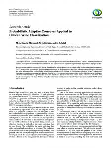
A genetic algorithm (GA) is one such versatile optimization method. Figure 1 shows the optimization process of a GA – the two primary operations are mating and mutation. The GA combines the best of the last generation through mating, in which parameter values are exchanged between parents to form offspring. Some of the parameters mutate [6]. The objective function then judges the fitness of the new sets of parameters and the algorithm iterates until it converges. With these two operators, the GA is able to explore the full cost surface in order to avoid falling into local minima. At the same time, it exploits the best features of the last generation to converge to increasingly better parameter sets.

The TSP can be modeled in a linear programming problem under constraints, as follows: We associate to each city a number between 1 and V. For each pair of cities (i, j), we define cij the transition cost from city i to the city j, and the binary variable: 𝑥𝑖𝑗 =

0

1 𝐼𝑓𝑡ℎ𝑒𝑡𝑟𝑎𝑣𝑒𝑙𝑒𝑟𝑚𝑜𝑣𝑒𝑠𝑓𝑟𝑜𝑚𝑐𝑖𝑡𝑦𝑖𝑡𝑜𝑐𝑖𝑡𝑦𝑗 (6) 𝑒𝑙𝑠𝑒

So the TSP problem can be formulated as a problem of integer linear programming, as follows:

𝑚𝑖𝑛

𝑛 𝑖=1

𝑖−1 𝑗 =1 𝑐𝑖𝑗

𝑥𝑖𝑗

Initialize population

Evaluate Cost

𝑖𝑗

2−

𝑖∈𝑆

Solution

Mutation

Selection

(7)

𝑥𝑖𝑗 = 2, ∀𝑖 ∈ 𝑁 = 1,2, … , 𝑛 (8) 𝑗 𝑆 𝑥𝑖𝑗

Yes

No

Crossover

Under the following constraints:

1−

Converge?

≥ 2 𝑓𝑜𝑟𝑒𝑎𝑐ℎ𝑆𝑁(9)

There are several deterministic algorithms; we mention the method of separation and evaluation and the method of cutting planes. The deterministic algorithm used to find the optimal solution, but its complexity is exponential order, and it takes a lot of memory space and it requires a very high computation time. In large size problems, this algorithm cannot be used.

Fig.1. Flowchart of optimization with a genetic algorithm GAs are remarkably robust and have been shown to solve difficult optimization problems that more traditional methods can not. Some of the advantages of GAs include:

 They are able to optimize disparate variables, whether they are inputs to analytic functions, experimental data, or numerical model output.

 They can optimize either real valued, binary variables, or integer variables.

Because of the complexity of the problem and the limitations of the linear programming approach, other approaches are needed.

 They can process a large number of variables.  They can produce a list of best variables as well as the

2.2 Approximation algorithm

 They are good at finding a global minimum rather than

Many problems of practical significance are NP-complete, yet they are too important to abandon merely because we don’t know how to find an optimal solution in polynomial time. Even if a problem is NP-complete, there may be hope. We have at least three ways to get around NP-completeness. First, if the actual inputs are small, an algorithm with exponential running time may be perfectly satisfactory. Second, we may be able to isolate important special cases that we can solve in polynomial time. Third, we might come up with approaches to find nearoptimal solutions in polynomial time (either in the worst case or the expected case). In practice, near-optimality is often good enough. We call an algorithm that returns near-optimal solutions an approximation algorithm. An approximate algorithm, like the Genetic Algorithms, Ant Colony [17] and Tabu Search [9], is a way of dealing with NPcompleteness for optimization problem. This technique does not guarantee the best solution. The goal of an approximation algorithm is to come as close as possible to the optimum value in a reasonable amount of time which is at most polynomial time.

single best solution. local minima.

 They can simultaneously sample various portions of a cost surface.

 They are easily adapted to parallel computation. Some disadvantages are the lack of viable convergence proofs and the fact that they are not known for their speed. As seen later in this chapter, speed can be gained by careful choice of GA parameters. Although mathematicians are concerned with convergence, often scientists and engineers are more interested in using a tool to find a better solution than obtained by other means. The GA is such a tool. These algorithms were modeled on the natural evolution of species. We add to this evolution concepts the observed properties of genetics (Selection, Crossover, Mutation, etc), from which the name Genetic Algorithm. They attracted the interest of many researchers, starting with Holland [15], who developed the basic principles of genetic algorithm, and Goldberg [8] has used these principles to solve a specific optimization problems. Other researchers have followed this path [10]-[14].

51

International Journal of Computer Applications (0975 – 8887) Volume 31– No.11, October 2011

3.1 Principles and Functioning

4.2 Generation of the initial population

Irrespective of the problems treated, genetic algorithms, presented in figure (Fig. 1), are based on six principles:  Each treated problem has a specific way to encode the individuals of the genetic population. A chromosome (a particular solution) has different ways of being coded: numeric, symbolic, or alphanumeric;  Creation of an initial population formed by a finite number of solutions;  Definition of an evaluation function (fitness) to evaluate a solution;  Selection mechanism to generate new solutions, used to identify individuals in a population that could be crossed, there are several methods in the literature, citing the method of selection by rank, roulette, by tournament, random selection, etc.;  Reproduce the new individuals by using Genetic operators: i. Crossover operator: is a genetic operator that combines two chromosomes (parents) to produce a new chromosome (children) with crossover probability Px ; ii. Mutation operator: it avoids establishing a uniform population unable to evolve. This operator used to modify the genes of a chromosome selected with a mutation probability Pm;  Insertion mechanism: to decide who should stay and who should disappear.  Stopping test: to make sure about the optimality of the solution obtained by the genetic algorithm. We presented the various steps which constitute the general structure of a genetic algorithm: Coding, method of selection, crossover and mutation operator and their probabilities, insertion mechanism, and the stopping test. For each of these steps, there are several possibilities. The choice between these various possibilities allows us to create several variants of genetic algorithm. Subsequently, our work focuses on finding a solution to that combinative problem: What are the best settings which create an efficient genetic variant to solve the Traveling Salesman Problem?

The initial population conditions the speed and the convergence of the algorithm. For this, we applied several methods to generate the initial population:  Random generation of the initial population.

4. APPLIED GENETIC ALGORITHMS TO THE TRAVELING SALESMAN PROBLEM 4.1 Problem representation methods In this section we will present the most adapted method of data representation, the path representation method, with the treated problem. The path representation is perhaps the most natural representation of a tour. A tour is encoded by an array of integers representing the successor and predecessor of each city. Table 2. Coding of a tour (3, 5, 2, 9, 7, 6, 8, 4) 3

5

2

9

7

6

8

4

 Generation of the first individual randomly, this one will be mutated N-1 times with a mutation operator. Generation of the first individual by using a heuristic mechanism. The successor of the first city is located at a distance smaller compared to the others. Next, we use a mutation operator on the route obtained in order to generate (N2) other individuals who will constitute the initial population.

4.3 Selection While there are many different types of selection, we will cover the most common type - roulette wheel selection. In roulette wheel selection, the individuals are given a probability Pi of being selected (10) that is directly proportionate to their fitness. The algorithm for a roulette wheel selection algorithm is illustrated in algorithm (Fig. 3) 1  N−1

1−

fi j∈Population

fj

(10)

Which fi is value of fitness function for the individual i. for all members of population sum += fitness of this individual endfor for all members of population probability = sum of probabilities + (fitness / sum) sum of probabilities += probability endfor number = Random between 0 and 1 for all members of population if number > probability but less than next probability then you have been selected endfor

Fig.2. Roulette wheel selection algorithm Thus, individuals who have low values of the fitness function may have a high chance of being selected among the individuals to cross.

4.4 Crossover Operator The search of the solution space is done by creating new chromosomes from old ones. The most important search process is crossover. Firstly, a pair of parents is randomly selected from the mating pool. Secondly, a point, called crossover site, along their common length is randomly selected, and the information after the crossover site of the two parent strings are swapped, thus creating two new children. Of course, this basic crossover method does not support for the TSP [18]. The two newborn chromosomes may be better than their parents and the evolution process may continue. The crossover in carried out according to the crossover probability Px.In this paper, we chose five crossover operators; we will explain their ways of proceeding in the following.

52

International Journal of Computer Applications (0975 – 8887) Volume 31– No.11, October 2011 Table 5. Example of PMX operator

4.4.1 Uniform crossover operator The child is formed by a alternating randomly between the two parents.

3

Parent 1 1 4 7

5

6

2

8

3

4

5

3

2

7

1

6

4

Child 1 1 8 6

2

7

2

8

4.4.2 Cycle Crossover The Cycle Crossover (CX) proposed by Oliver [15] builds offspring in such a way that each city (and its position) comes from one of the parents. We explain the mechanism of the cycle crossover using the following algorithm (Fig.3). Table 3. Cycle Crossover operator 1

2 *

Parent 1 3 4 5

6

7

4

2

Child 1 1 3 5

6

7

(G.XP.1) (G.XP.2)

* 7 5 1 Parent 1

3

2

6

4

1

5

3 4 2 Child 2

6

7

4 6 5 Parent 2

1

8

5 7 3 Child 2

Input: Parents x1=[x1,1,x1,2,……,x1,n] and x2=[x2,1,x2,2,……,x2,n] Output:Children y1=[y1,1,y1,2,……,y1,n] and y2=[y2,1,y2,2,……,y2,n] -----------------------------------------------------------------------------------Initialize  y1 = x1 and y2 = x2;  Initialize p1 and p2 the position of each index in y1 and y2;  Choose two crossover points a and b such that 1 ≤ a ≤ b ≤ n; for each i between a and b do t1 = y1,i and t2 = y2,i ; y1,i = t2 and y1,p1,t1 = t1 ; y2,i = t1 and y2,p2,t2 = t2 ; p1,t1= p1,t2 and p1,t2 = p1,t1 ; p2,t1 = p2,t2 and p2,t2 = p2,t1 ;

endfor Input: Parents x1=[x1,1,x1,2,……,x1,n] and x2=[x2,1,x2,2,……,x2,n] Output:Children y1=[y1,1,y1,2,……,y1,n] and y2=[y2,1,y2,2,……,y2,n] -----------------------------------------------------------------------------------Initialize  Initialize y1 and y2 being a empty genotypes; y1,1= x1,1; y2,1 = x2,1; i = 1; Repeat j ← Index where we find x2,i, in X1; y1,j = x1,j ; y2,j = x2,j ; i = j; Until x2,i y1 For each gene not yet initialized do y1,i = x2,i; y2,i = x1,i; Endfor

4.4.3 Partially-Mapped Crossover (PMX) Partially matched crossover PMX noted, introduced by Goldberg and Lingel [19], is made by randomly choosing two crossover points XP1 and XP2 which break the two parents in three sections. Table 4. The partition of a parent S2

4.4.4 The uniform partially-mapped crossover (UPMX) The Uniform Partially Matched Crossover presented by Cicirello and Smith [21], uses the technique of PMX. Any times, it does not use the crossover points; instead, it uses a probability of correspondence for each iteration. The algorithm (Fig.5) and the following example describe this crossover method. Table 6. UPMX operator example 3

5

Parent 1 1 4 7

4 6 5 Parent 2

Fig.3. Cycle Crossover (CX) algorithm

S1

Fig.4. PMXCrossover Algorithm

S3

S1 and S3 the sequences of Parent1 are copied to the Child1, the sequence S2 of the Child1 is formed by the genes of Parent2, beginning with the start of its part S2 and leaping the genes that are already established. The algorithm (Fig.4) shows the crossover method PMX.

1

8

6

2

8

5

6

1

3

2

7

4

3

6

Child 1 4 8 3

1 7 5 Child 2

2

7

2

8

Input: Parents x1=[x1,1,x1,2,……,x1,n] and x2=[x2,1,x2,2,……,x2,n] Output:Children y1=[y1,1,y1,2,……,y1,n] and y2=[y2,1,y2,2,……,y2,n] -----------------------------------------------------------------------------------Initialize  y1 = x1 and y2 = x2;  Initialize p1 and p2 the position of each index in y1 and y2;  Choose two crossover points a and b such that 1 ≤ a ≤ b ≤ n; For each i between 1 and n do Chose a random number q between 0 and 1; if q ≥ p then t1 = y1,i and t2 = y2,i ; y1,i = t2 and y1,p1,t1 = t1 ; y2,i = t1 and y2,p2,t2 = t2 ; p1,t1= p1,t2 and p1,t2 = p1,t1 ; p2,t1 = p2,t2 and p2,t2 = p2,t1 ; endif endfor

Fig.5. Algorithm of UPMXCrossover

53

International Journal of Computer Applications (0975 – 8887) Volume 31– No.11, October 2011

4.4.5 Non-Wrapping Ordered Crossover (NWOX)

Input: Parents x1=[x1,1,x1,2,……,x1,n] and x2=[x2,1,x2,2,……,x2,n] Output:Children y1=[y1,1,y1,2,……,y1,n] and y2=[y2,1,y2,2,……,y2,n] -----------------------------------------------------------------------------------Initialize  Initialize y1 and y2 being a empty genotypes;  Choose two crossover points a and b such that 1 ≤ a ≤ b ≤ n; j1 = j2 = k = b+1;

Non-Wrapping Ordered Crossover (NWOX) operator introduced by Cicirello [20], is based upon the principle of creating and filling holes, while keeping the absolute order of genes of individuals. The holes are created at the retranscription of the genotype, if xj,i {xk,a, . . . ,xk,b}then xj,i is a hole. The example (Table.7) and the algorithm (Fig.6) explain this technique:

i = 1; Repeat

Table 7. NWOX operator example 3

5

Parent 1 1 4 7

4 6 5 Parent 2

1

8

6

2

8

3

4

5

3

2

7

6

5

1

Child 1 1 8 7

4 7 8 Child 2

6

2

3

2

if x1,i {x2,a, . . . ,x2,b} then y1,j1 = x1,k ;j1++; if x2,i {x1,a, . . . ,x1,b} theny2,j1 = x2,k ;j2++; k=k+1;

Until i ≤ n y1 = [y1,1 ……y1,a−1 x2,a ……x2,b y1,a ……y1,n−a]; y2 = [y2,1 ……y2,a−1 x1,a ……x1,b y2,a ……y2,n−a];

Fig 7. Algorithm of Crossover operator OX Input: Parents x1=[x1,1,x1,2,……,x1,n] and x2=[x2,1,x2,2,……,x2,n] Output:Children y1=[y1,1,y1,2,……,y1,n] and y2=[y2,1,y2,2,……,y2,n] -----------------------------------------------------------------------------------Initialize  Initialize y1 and y2 being a empty genotypes;  Choose two crossover points a and b such that 1 ≤ a ≤ b ≤ n; y1,1= x1,1; y2,1 = x2,1; i = 1;

4.4.7 Crossover with reduced surrogate The reduced surrogate operator constrains crossover to always produce new individuals wherever possible. This is implemented by restricting the location of crossover points such that crossover points only occur where gene values differ.

4.4.8 Shuffle crossover Shuffle crossover is related to uniform crossover. A single crossover position (as in single-point crossover) is selected. But before the variables are exchanged, they are randomly shuffled in both parents. After recombination, the variables in the offspring are unstuffed. This removes positional bias as the variables are randomly reassigned each time crossover is performed.

for each i between a and n do ifx1,i {x2,a, . . . ,x2,b} then y1 = [y1 x1,i] ; ifx2,i {x1,a, . . . ,x1,b} then y2 = [y2 x2,i] ; endfor y1 = [y1,1 ……y1,a−1 x2,a ……x2,b y1,a ……y1,n−a]; y2 = [y2,1 ……y2,a−1 x1,a ……x1,b y2,a ……y2,n−a];

4.5 Mutation Operators

Fig 6.Algorithm of NWOXcrossover operator

The two individuals (children) resulting from each crossover operation will now be subjected to the mutation operator in the final step to forming the new generation. This operator randomly flips or alters one or more bit values at randomly selected locations in a chromosome.

4.4.6 Ordered Crossover (OX) The Ordered Crossover method is presented by Goldberg[8], is used when the problem is of order based, for example in Ushaped assembly line balancing etc. Given two parent chromosomes, two random crossover points are selected partitioning them into a left, middle and right portion. The ordered two-point crossover behaves in the following way: child1 inherits its left and right section from parent1, and its middle section is determined.

The mutation operator enhances the ability of the GA to find a near optimal solution to a given problem by maintaining a sufficient level of genetic variety in the population, which is needed to make sure that the entire solution space is used in the search for the best solution. In a sense, it serves as an insurance policy; it helps prevent the loss of genetic material.

Table 8. OX operator example 3

5

Parent 1 1 4 7

4 6 5 Parent 2

1

8

6

2

8

4

7

5

3

2

7

5

8

1

Child 1 1 8 6

4 7 3 Child 2

In this study, we chose as mutation operator the Mutation methodReverse Sequence Mutation (RSM). 2

3

2

6

In the reverse sequence mutation operator, we take a sequence S limited by two positions i and j randomly chosen, such that i