A Comparative Study of Algorithmic Debugging Strategies? Josep Silva DSIC, Technical University of Valencia Camino de Vera s/n, E-46022 Valencia, Spain
[email protected]
Abstract. Algorithmic debugging is a debugging technique that has been extended to practically all programming paradigms. It is based on the answers of the programmer to a series of questions generated automatically by the algorithmic debugger. Therefore, the performance of the technique is strongly dependent on the number and the complexity of these questions. In this work we overview and compare current strategies for algorithmic debugging and we introduce some new strategies and discuss their advantages over previous approaches.
1
Introduction
Algorithmic debugging is a debugging technique which relies on the programmer having an intended interpretation of the program. In other words, some computations of the program are correct and others are wrong with respect to the programmer’s intended semantics. Therefore, algorithmic debuggers compare the results of sub-computations with what the programmer intended. By asking the programmer questions or using a formal specification the system can identify precisely the location of a program’s bug. Essentially, algorithmic debugging is a two-phase process: An execution tree (see, e.g., [12]), ET for short, is built during the first phase. Each node in this ET corresponds to an equation which consists of a function call with completely evaluated arguments and results1 . Roughly speaking, the ET is constructed as follows: The root node is the main function of the program; for each node n with associated function f , and for each function call in the right-hand side of the definition of f , a new node is recursively added to the ET as the child of n. This notion of ET is valid for functional languages but it is insufficient for other paradigms as the imperative programming paradigm. In general, the information included in the nodes of the ET incudes all the data needed to determine if the equations are correct. For instance, in the imperative programming paradigm, ?
1
This work has been partially supported by the EU (FEDER) and the Spanish MEC under grant TIN2005-09207-C03-02, by the ICT for EU-India Cross-Cultural Dissemination Project ALA/95/23/2003/077-054, and by the Vicerrectorado de Innovaci´ on y Desarrollo de la UPV under project TAMAT ref 5771. Or as much as needed if we consider a lazy language.
with the function (or procedure) of each node it is included the value of all global variables when the function was called. Similarly, in object-oriented languages, every node with a method invocation includes the values of the attributes of the object owner of this method (see, e.g., [4]). In the second phase, the debugger traverses the ET asking an oracle (typically the programmer) whether each equation is correct or wrong. At the beginning, the suspicious area which contains those nodes that can be buggy (a buggy node is associated with a buggy rule of the program) is empty; but, after every question, some nodes of the ET leave the suspicious area. When all the children of a node with a wrong equation (if any) are correct, the node becomes buggy and the debugger locates the bug in the function definition of this node [14]. If a bug symptom is detected then algorithmic debugging is complete [16]. It is important to say that, once the execution tree is built, the problem of traversing it and selecting a node is independent of the language used; hence algorithmic debugging strategies can theoretically work for any language. Unfortunately, in practice—for real programs—algorithmic debugging can produce long series of questions which are semantically unconnected (i.e., consecutive questions which refer to different and independent parts of the computation) making the process of debugging too complex. Furthermore, questions can also be very complex. For instance, during a debugging session with a compiler, the algorithmic debugger of the Mercury language [10]—currently, one of the most advanced algorithmic debuggers—asked a question of more than 1400 lines. Therefore, new techniques and strategies to reduce the number of questions, to simplify them and to improve the order in which they are asked are a necessity to make algorithmic debuggers usable in practice. In this paper we review and compare the current algorithmic debugging strategies and propose three new strategies (less YES first, divide by YES and query, and dynamic weighting search) that can further reduce the number of questions asked during an algorithmic debugging session. The rest of the paper is organized as follows. The next section shows an example of algorithmic debugging session that will be used along the paper. Section 3 reviews current algorithmic debugging strategies and proposes three new strategies. In Section 4 we present a comparison of all techniques and we study their costs. Finally, Section 5 concludes.
2
Algorithmic Debugging
During the algorithmic debugging process, an oracle is prompted with equations and asked about their correctness; it answers “YES” when the result is correct or “NO” when the result is wrong. Some algorithmic debuggers also accept the answer “I don’t know” when the programmer cannot give an answer (e.g., because the question is too complex). After every question, some nodes of the ET leave the suspicious area. When there is only one node in the suspicious area, the process finishes reporting this node as buggy. It should be clear that 2
algorithmic debugging finds one bug at a time. In order to find different bugs, the process should be restarted again for each different bug. main = sqrtest [1,2] sqrtest x = test (computs (listsum x)) test (x,y,z) = (x==y) && (y==z) listsum [] = 0 listsum (x:xs) = x + (listsum xs) computs x = ((comput1 x),(comput2 x),(comput3 x)) comput1 x = square x square x = x*x comput2 x = listsum (list x x) list x y | y==0 = [] | otherwise = x:list x (y-1) comput3 x = listsum (partialsums x) partialsums x = [(sum1 x),(sum2 x)] sum1 x = div (x * (incr x)) 2 sum2 x = div (x + (decr x)) 2 incr x = x + 1 decr x = x - 1
Fig. 1. Example program
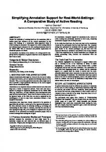
Let us illustrate the process with an example2 . Example 1. Consider the buggy program in Fig. 1 adapted to Haskell from [7]. This program sums a list of integers [1,2] and computes the square of the result with three different methods. If the three methods compute the same result the program returns T rue; otherwise, it returns F alse. Here, one of the three methods—the one adding the partial sums of its input number—contains a bug. From this program, an algorithmic debugger can automatically generate the ET 2
While almost all the strategies presented here are independent of the programming paradigm used, in order to be concrete and w.l.o.g. we will base our examples on the functional programming paradigm.
3
Fig. 2. Execution tree of the program in Fig. 1
4
(6) square 3 = 9
(12) list 3 3 = [3,3,3]
(13) list 3 2 = [3,3]
(14) list 3 1 = [3]
(15) list 3 0 = []
(9) listsum [3,3] = 6
(10) listsum [3] = 3
(11) listsum [] = 0
(7) comput2 3 = 9
(19) listsum [] = 0
(18) listsum [2] = 2
(17) listsum [6,2] = 8
(16) comput3 3 = 8
(4) computs 3 = (9,9,8)
(8) listsum [3,3,3] = 9
(5) comput1 3 = 9
(3) test (9,9,8) = False
(2) sqrtest [1,2] = False
(1) main = False
(22) incr 3 = 4
(21) sum1 3 = 6
(27) listsum [] = 0
(24) decr 3 = 2
(23) sum2 3 = 2
(26) listsum [2] = 2
(20) partialsums 3 = [6,2]
(25) listsum [1,2] = 3
Starting Debugging Session... (1) (2) (3) (4) (5) (7) (16) (17) (20) (21) (23) (24)
main = False? NO sqrtest [1,2] = False? NO test [9,9,8] = False? YES computs 3 = [9,9,8]? NO comput1 3 = 9? YES comput2 3 = 9? YES comput3 3 = 8? NO listsum [6,2] = 8? YES partialsums 3 = [6,2]? NO sum1 3 = 6? YES sum2 3 = 2? NO decr 3 = 2? YES
Bug found in rule: sum2 x = div (x + (decr x)) 2
Fig. 3. Debugging session for the program in Fig. 1
of Fig. 2 (for the time being, the reader can ignore the distinction between different shapes and white and dark nodes) which, in turn, can be used to produce a debugging session as depicted in Fig. 3. During the debugging session, the system asks the oracle about the correctness of some ET nodes w.r.t. the intended semantics. At the end of the debugging session, the algorithmic debugger determines that the bug of the program is located in function “sum2” (node 23). The definition of function “sum2” should be: sum2 x = div (x*(decr x)) 2
3
Algorithmic Debugging Strategies
Algorithmic debugging strategies are based on the fact that the ET can be pruned using the information provided by the oracle. Given a question associated with a node n of the ET, a NO answer prunes all the nodes of the ET except the subtree rooted at n; and a YES answer prunes the subtree rooted at n. Each strategy takes advantage of this property in a different manner. A correct equation in the tree does not guarantee that the subtree rooted at this equation is free of errors. It can be the case that two buggy nodes caused the correct answer by fluke [6]. In contrast, an incorrect equation does guarantee that the subtree rooted at this equation does contain a buggy node [12]. Therefore, if a program produced a wrong result, then the equation in the root of the ET is wrong and thus there must be at least one buggy node in the ET. We will assume in the following that the debugging session has been started after discovering a bug symptom in the output of the program, and thus the root of the tree contains a wrong equation. Hence, we know that there is at least one bug in the program. 5
We will also assume that the oracle is able to answer all the questions. Then, all the strategies will find the bug. 3.1
Single Stepping (Shapiro, 1982)
The first algorithmic debugging strategy to be proposed was single stepping [16]. In essence, this strategy performs a bottom-up search because it proceeds by doing a post-order traversal of the ET. It asks first about all the children of a given node, and then (if they are correct) about the node itself. If the equation of this node is wrong then this is the buggy node; if it is correct, then the postorder traversal continues. Therefore, the first node answered NO is identified as buggy (because all its children have already been answered YES). For instance, the sequence of 19 questions asked for the ET in Fig. 2 would be: 3-YES, 6-YES, 5-YES, 11-YES, 10-YES, 9-YES, 8-YES, 15-YES, 14-YES, 13-YES, 12-YES, 7-YES, 19-YES, 18-YES, 17-YES, 22-YES, 21-YES, 24-YES, 23-NO. Note that in this strategy questions are semantically unconnected. 3.2
Top-Down Search (Av-Ron, 1984)
Due to the fact that questions are asked in a logical order, top-down search [1] is the strategy that has been traditionally used (see, e.g., [3, 9]) to measure the performance of different debugging tools and methods. It basically consists in a top-down, left-to-right traversal of the ET and, thus, the node asked is always a child or a sibling of the previous question node. When a node is answered NO, one of its children is asked; if it is answered YES, one of its siblings is. Therefore, the idea is to follow the path of wrong equations from the root of the tree to the buggy node. For instance, the sequence of 12 questions asked for the ET in Fig. 2 is shown in Fig. 3. This strategy significantly improves single stepping because it prunes a part of the ET after every answer. However, it is still very naive, since it does not take into account the structure of the tree (e.g., how balanced it is). For this reason, a number of variants aiming at improving it can be found in the literature: Top-Down Zooming (Maeji and Kanamori, 1987) During the search of previous strategies, the rule or indeed the function definition may change from one query to the next. If the oracle is human, this continuous change of function definitions slows down the answers of the programmer because he has to switch thinking once and again from one function definition to another. This drawback can be partially overcome by changing the order of the questions: In this strategy [11], recursive child calls are preferred. The sequence of questions asked for the ET in Fig. 2 is exactly the same as with top-down search (Fig. 3) because no recursive calls are found. Another variant of this strategy called exception zooming, introduced by Ian MacLarty [10], selects first those nodes that produced an exception at runtime. 6
Heaviest First (Binks, 1995) Selecting always the left-most child does not take into account the size of the subtrees that can be explored. Binks proposed in [2] a variant of top-down search in order to consider this information when selecting a child. This variant is called heaviest first because it always selects the child with a bigger subtree. The objective is to avoid selecting small subtrees which have a lower probability of containing the bug. For instance, the sequence of 9 questions asked for the ET in Fig. 2 would be3 : 1-NO, 2-NO, 4-NO, 7-YES, 16-NO, 20-NO, 21-YES, 23-NO, 24-YES. Less YES First (Silva, 2006) This section introduces a new variant of topdown search which further improves heaviest first. It is based on the fact that every equation in the ET is associated with a rule of the source code (i.e., the rule that the debugger identifies as buggy when it finds a buggy node in the ET). Taking into account that the final objective of the process is to find the program’s rule which contains the bug—rather than a node in the ET—and considering that there is not a relation one-to-one between nodes and rules because several nodes can refer to the same rule, it is important to also consider the node’s rules during the search. A first idea could be to explore first those subtrees with a higher number of associated rules (instead of exploring those subtrees with a higher number of nodes). Example 2. Consider the following ET: 1
2
3
4
5
6
8
7
8
8
7
where each node is labeled with its associated rule and where the oracle answered NO to the question in the root of the tree. While heaviest first selects the rightmost child because this subtree has four nodes instead of three, less YES first selects the left-most child because this subtree contains three different rules instead of two. Clearly, this approach relies on the idea that all the rules have the same probability of containing the bug (rather than all the nodes). Another possibility could be to associate a different probability of containing the bug to each rule, e.g., depending on its structure: Is it recursive? Does it contain higher-order calls?. The probability of a node to be buggy is q · p where q is the probability that the rule associated to this node is wrong, and p is the probability of this rule to 3
Here, and in the following, we will break the indeterminism by selecting the left-most node in the figures. For instance, the fourth question could be either (7) or (16) because both have a weight of 9. We selected (7) because it is on the left.
7
execute incorrectly. Therefore, under the assumption that all the rules have the same probability of being wrong, the probability P of a branch b to contain the Pn pi where n is the number of nodes in b, R is the number of rules bug is P = i=1 R in the program, and pi is the probability of the rule in node i to produce a wrong result if it is incorrect. Clearly, if wePassume that a wrong rule always produces r pi a wrong result4 we have that P = i=1 and ∀i.pi = 1, then the probability R r where r is the number of rules in b, and thus, this strategy is (on average) is R better than heaviest first. For instance, in Example 2 the left-most branch has a probability of 38 to contain a buggy node, while the right-most branch has a probability of 28 despite it has more nodes. However, in general, a wrong rule can produce a correct result, and thus we need to consider the probability of a wrong rule to return a wrong answer. This probability has been approximated by the debugger Hat-delta (see Section 3.4) by using previous answers of the oracle. The main idea is that a rule answered NO n times out of m is more likely to be wrong than a rule answered NO n0 times out of m if n0 < n 6 m. Here, we use this idea in order to compute the probability of a branch to contain a buggy node. Hence, this strategy is a combination of the ideas from both heaviest first and Hat-delta. However, while heaviest first considers the structure of the tree and does not take into account previous answers of the user, Hat-delta does the opposite; thus, the advantage of less YES first over them is the use of more information (both the structure of the tree and previous answers of the user). A direct generalization of Hat-delta for branches would result in counting the number of YES answers of a given branch; but this approach would not take into account the number of rules in the branch. In contrast, we proceed as follows: When a node is set correct, we mark its associated rule and all the rules of its descendants as correctly executed. If a rule has been executed correctly before, then it will likely execute correctly again. The debugger associates to each rule of the program the number of times it has been executed in correct computations based on previous answers. Then, when we have to select a child to ask, we can compute the total number of rules in the subtrees rooted at the children, and the total number of answers YES for every rule. This strategy selects the child whose subtree is less likely to be correct (and thus more likely to be wrong). To compute this probability we calculate for every branch b a weight wb with the following equation: wb =
4
n X
1
(Y ES) i=1 ri
This assumption is valid for instance in those flattened functional languages where all the conditions in the right-hand side of function definitions have been distributed between its rules. This is relatively frequent in internal languages of compilers, but not in source languages.
8
(Y ES)
where n is the number of nodes in b and ri is the number of answers YES for the rule r of the node i. As with heaviest first, we select the branch with the biggest weight, the difference is that this equation to compute the weight takes into account previous answers of the user. Moreover, we assume that initially all the rules have been answered YES once, and thus, at the beginning, this strategy asks those branches with more nodes, but it becomes different as the number of questions asked increases. With this strategy, the sequence of 9 questions asked for the ET in Fig. 2 is: 1-NO, 2-NO, 4-NO, 7-YES, 16-NO, 20-NO, 21-YES, 23-NO, 24-YES. 3.3
Divide & Query (Shapiro, 1982)
In 1982, together with single stepping, Shapiro proposed another strategy: the so-called divide & query (D&Q) [16]. The idea of D&Q is to ask in every step a question which divides the remaining nodes in the ET by two, or, if this is not possible, into two parts with a weight as similar as possible. In particular, the original algorithm by Shapiro always chooses the heaviest node whose weight is less than or equal to w/2 where w is the weight of the suspicious area in the ET. This strategy has a worst case query complexity of order b log2 n where b is the average branching factor of the tree and n its number of nodes. This strategy works well with a large search space—this is normally the case of realistic programs—because its query complexity is proportional to the logarithm of the number of nodes in the tree. If the ET is big and unbalanced this strategy is better than top-down search [3]; however, the main drawback of this strategy is that successive questions may have no connection, from a semantic point of view, with each other; requiring the programmer more time for answering the questions. For instance, the sequence of 6 questions asked for the ET in Fig. 2 is: 7-YES, 16-NO, 17-YES, 21-YES, 24-YES, 23-NO. Hirunkitti’s Divide & Query (Hirunkitti and Hogger, 1993) In [8], Hirunkitti and Hogger noted that Shapiro’s algorithm does not always choose the node closest to the halfway point in the tree and addressed this problem slightly modifying the original divide & query algorithm. Their version of divide & query is the same as the one of Shapiro except that their version always chooses a node which produces a least difference between: – w/2 and the heaviest node whose weight is less than or equal to w/2 – w/2 and the lightest node whose weight is greater than or equal to w/2 where w is the weight of the suspicious area in the computation tree. For instance, the sequence of 6 questions asked for the ET in Fig. 2 is: 7-YES, 16-NO, 17-YES, 21-YES, 24-YES, 23-NO. 9
Biased Weighting Divide & Query (MacLarty, 2005) MacLarty proposed in his PhD thesis [10] that not all the nodes should be considered equally while dividing the tree. His variant of D&Q divides the tree by only considering some kinds of nodes and/or by associating a different weight to every kind of node. In particular, his algorithmic debugger was implemented for the functional logic language Mercury [5] which distinguishes between 13 different node types.
Divide by YES & Query (Silva, 2006) The same idea used in less YES first can be applied in order to improve divide & query. Instead of dividing the ET into two subtrees with a similar number of nodes, we can divide it into two subtrees with a similar weight. The problem that this strategy tries to address is the D&Q’s assumption that all the nodes have the same probability of containing the bug. In contrast, this strategy tries to compute this probability. By using the equation to compute the weight of a branch, this strategy computes the weight associated to the subtree rooted at each node. Then, the node which divides the tree into two subtrees with a more similar weight is selected. In particular, the node selected is the node which produces a least difference between: – w/2 and the heaviest node whose weight is less than or equal to w/2 – w/2 and the lightest node whose weight is greater than or equal to w/2 where w is the weight of the suspicious area in the ET. As with D&Q, different nodes could divide the ET into two subtrees with a similar weights; in this case, we could follow another strategy (e.g., Hirunkitti) in order to select one of them. We assume again that initially all the rules have been answered YES once. Therefore, at the beginning this strategy is similar to D&Q, but the differences appear as the number of answers increases. Example 3. Consider again the ET in Example 2. Similarly to D&Q, the first node selected is the top-most “8” because only structural information is available. Let us assume that the answer is YES. Then, we mark all the nodes in this branch as correctly executed. Therefore, the next node selected is “2”; because, despite the subtrees rooted at “2” and “5” have the same number of nodes and rules, we now have more information which allows us to know that the subtree rooted at “5” is more likely to be correct since node “7” has been correctly executed before. The main difference with respect to D&Q is that divide by YES & query not only takes into account the structure of the tree (i.e., the distribution of the program rules between its nodes), but also previous answers of the user. With this strategy, the sequence of 5 questions asked for the ET in Fig. 2 is: 7-YES, 16-NO, 21-YES, 23-NO, 24-YES. 10
3.4
Hat-delta (Davie and Chitil, 2005)
Hat [19] is a tracer for Haskell. Davie and Chitil introduced a declarative debugger tool based on the Hat’s traces that includes a new strategy called Hat-delta [6]. Initially, Hat-delta is identical to top-down search but it becomes different as the number of questions asked increases. The main idea of this strategy is to use previous answers of the oracle in order to compute which node has an associated rule that is more likely to be wrong (e.g., because it has been answered NO more times than the others). This strategy assumes that a rule answered NO n times out of m is more likely to be wrong than a rule answered NO n0 times out of m if n0 < n 6 m. During a debugging session, a sequence of questions, each of them related to a particular rule, is asked. In general, after every question, it is possible to compute the total number of questions asked for each rule, the total number of answers YES/NO, and the total number of nodes associated with this rule. Moreover, when a node is set correct or wrong, Hat-delta marks all the rules of its descendants as correctly or incorrectly executed respectively. This strategy uses all this information to select the next question. In particular, three different heuristics have been proposed based on this idea [6]: – Counting the number of YES answers. If a rule has been executed correctly before, then it will likely execute correctly again. The debugger associates to each rule of the program the number of times it has been executed in correct computations based on previous answers. – Counting the number of NO answers. This is analogous to the previous heuristic but collecting wrong computations. – Calculating the proportion of NO answers. This is derived from the previous two heuristics. For a node with associated rule r we have: number of answers NO for r number of answers NO/YES for r If r has not been asked before a value of
1 2
is assigned.
Example 4. Consider this program: 4|0|0 8|4| 13 4|0|0 4|0|0 0|0| 12
sort [] = [] sort (x:xs) = insert x (sort xs) insert x [] = [x] insert x (y:ys) | x