International Conference on Civil Engineering Architecture and urban infrastructure 29-30 July 2015, Tabriz, Iran
A comparative study of honey-bee mating optimization algorithm and support vector regression system approach for river discharge prediction Case study: Kashkan River Basin Hossein Foroozand, Seied Hosein Afzali*
1. MSc. in Civil Eng., Civil Eng. Dept., Eng. School, Shiraz University, Shiraz, Iran. E-mail:
[email protected]. 2. Assistant prof., Civil Eng. Dept., Eng. School, Shiraz University, Shiraz, Iran. (Corresponding author) E-mail:
[email protected]
Abstract Accurate forecasting of river flow is an important aspect of water resource planning and management especially in water scarce areas of developing countries. In this study, application of the honey bee mating optimization algorithm in comparison with a robust data-driven method such as support vector regression (SVR) assessed and proved to be an efficient forecasting tool for developing water resource programs. In order to achieve this purpose, four key factors such as antecedent daily river flow, soil infiltration rate, daily potential evapotranspiration and average daily precipitation were used to develop the models. The training and verification data sets were allocated respectively from 75% and 25% of an 18 year river flow, precipitation and temperature data series which were available from years 1993 to 2011. Three quantitative standard statistical performance evaluation measures of root mean squared error (RMSE), correlation coefficient (CC) and regressive coefficient (R2) were employed to evaluate the performances of the models. The best-fit model performance indicators, RMSE, CC and R2 returned values within the ranges 18.05–32.24, 0.86–0.96 and 0.6–0.89 respectively, considering both calibration and verification data for the two mentioned methods. A comprehensive comparison of the overall performance indicated that the HBMO model performed better than SVR in river flow forecasting for the verification period.
Keywords: River discharge prediction, Honey-bee mating optimization, Support vector regression, Kashkan River. 1
International Conference on Civil Engineering Architecture and urban infrastructure 29-30 July 2015, Tabriz, Iran
1. Introduction River discharge prediction has significant effect on water resource system planning and management, especially in dry areas where water resources are insufficient. Therefore, how to precisely forecast the river discharge based on measured records at a specified flow domain becomes a crucial issue from both academic and practical standpoints [1]. Due to this importance, river flow prediction methods have been studied by different scientists during the past few years. The river flow models can be divided into two main types, physical or conceptual based models and data-driven models [2]. The physically based models can be extremely complex. They often need some advanced mathematical tools and a significant amount of calibration data [2], while data-driven models do not need any information about the physics of the hydrologic processes. Therefore, they are very useful for river discharge prediction where the main concern is accurate predictions of runoff [3, 4 and 5]. Recently, some data-driven methods, such as artificial neutral networks (ANNs), adaptive neuro fuzzy inference system (ANFIS) and support vector machine (SVM) have been widely used for solving and stimulating the computational problems. These methods offer superiority over conventional modeling. He et al. [6] compared the performance of ANN, ANFIS and SVM methods for forecasting river flow in a semiarid mountainous region. They found that the SVM performed better than the other models. Also Kisi and Cimen [7] accepted that the SVM is a good soft computational technique for monthly stream flow forecasting. SVR is a new version of the SVM method. The theory of SVM is introduced by Vapnik [8]. This forecasting tool maximizes predictive accuracy while automatically avoiding over-fitting to the data [8]. SVM is used to solve the classification problem. The SVM implements the structural risk minimization (SRM) principle instead of the traditional empirical risk minimization (ERM) principle [9, 10]. The ERM principle can only minimize the training error. However, the SRM minimizes an upper bound of the generalization error. Therefore, The SVM model can obtain an optimum network structure and better generalization using the SRM principle [11]. Vapnik [8] proposed another version of SVM for solving the regression problem. This new version is called support vector regression (SVR), which has become the most commonly applied form of SVM. The SVR method has extensive usage in several hydrological applications. Liong and Sivapragasam [12] used a SVR for flood stage forecasting in Dhaka, Bangladesh. Bray and Han [13] identified an appropriate model structure and relevant parameters when using SVR to accurately forecast stream flows. Jayawardena et al. [14] worked on logic systems approach for river discharge prediction. Liu et al. [15] applied coupled discrete wavelet transform and SVR for daily and monthly stream flow forecasting. Kalteh [16] predicted monthly discharge by using wavelet-based data-driven models including SVR.
2
International Conference on Civil Engineering Architecture and urban infrastructure 29-30 July 2015, Tabriz, Iran
More recently, HBMO algorithm have shown a significant potential and good perspective for the solution of various optimization problems. The HBMO algorithm has outstanding accuracy and calculation speed to deal with the optimization problem. Advantages of the HBMO algorithm are presented in some previous researches [17, 18, 19]. Niazkar and Afzali [20] used HBMO algorithm for optimum design of lined channel sections .Moreover. Niazkar and Afzali [21] presented the application of the modified honey bee mating optimization for Parameter estimation of nonlinear Muskingum model. Jahromi and Afzali [22] proposed the application of the HBMO approach to predict the total-sediment discharge. In this study, at first a new empirical model is proposed for the river discharge prediction on the basis of HBMO algorithm. Furthermore, the performance of the developed model is evaluated through detailed comparisons with the SVR method as a competitive alternative which is already proved to be one of the most advantageous approaches among other mentioned data-driven methods. In order to analyze the performance and accuracy of these two methods, the HBMO and SVR models are applied to predict the Kashkan River's discharge located in Lorestan province of western region of Iran. Statistical analysis of the results showed high efficacy and reliability of the proposed HBMO method and its superiority over SVR method on the basis of better performance and accuracy confirmed through comparative analysis.
2. Methodology 2.1. Support vector regression (SVR( It is generally accepted that SVM can be used as an extremely robust and efficient algorithm for the classification [8] and regression problems [23]. The main objective of SVM classification is to build decision boundaries in the characteristic space which separate data points belonging to different types. In the meanwhile, SVR is derived from the SVM [8]. SVR is widely applied to solve the regression problems. SVR uses a hypothesis space of linear functions in a highdimensional characteristic space [9]. The regression function of SVR is formulated as follows: xi x1i , x2i ,..., xmi , yi y1 , y 2 ,..., y n ,
i 1,..., n i 1,..., n
f ( x) (w.( x)) b
(1) (2)
(3) Where 𝑥𝑖 includes the m input vector of the sample and 𝑦𝑖 represents the output target and n is the total number of data points. The w and b are the coefficients of the regression function. While Ф(𝑥) is a nonlinear mapping function. By mapping the input vector to a high-dimensional space, the nonlinear separable problem becomes linearly separable in space [24]. The coefficients of a traditional regression model are derived by minimizing the square error, which are represented an
3
International Conference on Civil Engineering Architecture and urban infrastructure 29-30 July 2015, Tabriz, Iran
empirical risk based on the loss function [25]. The SVR uses a new type of loss function, called the 𝜀-insensitivity loss function (𝐿𝜀 ), which is defined as below: f x y for f x y L f x , y 0 otherwise (4) Where 𝜀 is a parameter assumed by the user. There is no loss when the predicted output falls into the band area. On the other hand, if the predicted output falls out the band area, the loss is equal to the difference between the predicted value and the margin [25]. Using the SRM principle, the coefficient, w, in Eq. (3) can be calculated by minimizing the following regularized risk function: 1 n 1 2 (5) Rreg C L f xi , y i w n i 1 2 1 2 Where w denotes the adjustment term that determines the tradeoff between the complexity and 2 the approximation accuracy of the regression model and ensures the model possesses an improved generalized performance, and C is a constant parameter which assumed by user that influences the tradeoff between the regularization term and the empirical risk [15]. The following objective function is solved to estimate the linear regression in SVR (Vapnik, 1995): n 1 2 (6) min w C i i 2 i 1
yi w.xi b i subjected to w.xi b y i i i 0, i 0, i 1,..., n Where i
(7)
and i are positive variables, serving as a measure of training samples outside the 𝜀-
insensitivity area and C is a positive constant influencing the degree of penalizing loss when a training error occurs. Eq. (6) is a quadratic programming problem, which can be estimated by using Lagrangian theory and the Karush–Kühn–Tucker condition [26, 27]. The general formulation of the SVR function is [25]: n
f x i i K x, xi b
(8)
(9)
i 1
K x, xi exp x xi
2
Where 𝛼𝑖 and 𝛼𝑖∗ are the Lagrangian multipliers and K(x, xi) is the Kernel function, and 𝛾 is the Kernel specific parameter. Kernel functions change the dimensionality of the input space [27] (Azamathulla and Wu, 2011). The kernel function plays an important role in SVR and its 4
International Conference on Civil Engineering Architecture and urban infrastructure 29-30 July 2015, Tabriz, Iran
performance. While there are several choices for the Kernel function (e.g., linear, polynomial, radial basis function (RBF), multi-layer perception, etc.), in the current study, the radial basis function is used. In this study, the SVR parameters are optimized by implementing a two-step grid search method. This can calibrate the parameters more effectively and systematically than the traditional method [28]. The first step applies a coarse grid to determine the ‘‘better’’ region of the grid. A finer grid search on this ‘‘better’’ region is then conducted to find the optimal parameters. Detailed information about this optimization method and the SVR model is given by Hsu et al. [28]. We implement the SVR models based on the LIBSVM program developed by Chang and Lin [29]. In this study, the m (=7) input vector refers to the one, two, three and four antecedent daily river flow values, soil infiltration rate, daily potential evapotranspiration and average daily precipitation in the river basin, and the output target refers to daily discharge and n is the number of samples in the training dataset which equals to 5202 in the present study. 2.2. HBMO Algorithm The honey bee is one of the sociable species that can survive only as a member of a community, or colony. Every colony typically has a single egg-laying long-lived queen, something about zero to several thousand drones (depending on the season) and usually 10,000 to 60, 000 workers [30]. Queens are specialized in egg laying [31]. Colonies are divided in two types monogynous and polygynous which have one queen or more during its life-cycle, respectively. The queen bee only eats royal jelly, which is a milky-white colored, jelly-like substance. Nurse bees generate this valuable food from their glands, and feed it to their queen. The queen became the biggest bee in colony because of this special diet. A queen bee has a life span between five or six years, while worker bees and drones live less than 6 months. The drone population is usually something around several hundred in a hive. The drones have just one task, which is to present the best possible sperm to the queen in mating flight. Drones are regarded as amplifying factors that transfer their mothers’ genome without changing their genetic composition. As a result, drones are considered as agents that offspring one of their mother’s gametes. Brood care is the most important role of worker bees but sometimes they lay eggs. However, the worker’s eggs are unfertilized. In the marriage flight, the queen mates during its mating flights far from the nest. In each mating, queen selectively chooses the best sperm and then accumulates them to form the genetic pool. In laying eggs, queen randomly chooses a mixture of the sperm accumulated in the spermatheca to fertilize the egg. The HBMO Algorithm mixes a number of different maneuvers [17, 18].. Each of them is related to a different phase of the mating process of the honey bee. A drone mates with a queen probabilistically using an annealing function as follows:
5
International Conference on Civil Engineering Architecture and urban infrastructure 29-30 July 2015, Tabriz, Iran
f (10) probD exp st Where Prop (D) is the probability of choosing the sperm of drone D to the spermtheca of the queen, Δ(f) is the absolute difference between the fitness of D and the fitness of the queen and S(t) is the queen’s speed at time (t). This function is named as an annealing function, in which the mating probability is high when either the queen’s spermatheca is in the beginning of the mating flight or when the drone’s fitness is good. After each perfect mating, the queen’s speed, S(t) and energy, E(t), decline by using the following equations:
S t 1 S t
(11)
Et 1 Et
(12) Where α is a reduction factor ∈ (0, 1) and 𝛾 is the amount of energy reduction after each perfect mating. Initially, the speed of the queen is generated randomly. A number of mating flights are computed. Therefore, HBMO algorithm has the following five main stages [32]: 1. The algorithm starts with the mating flight, where a queen (best solution) selects drones probabilistically to form the spermtheca. 2. One drone is randomly selected for the creation of broods. 3. Producing of new broods (trial solutions). 4. Workers conduct local search on new broods (trial solutions). 5. Adjustment of workers’ fitness based on the amount of improvement achieved on broods. 6. Comparing between the queen and the best brood and replacement of weaker queens by fitter broods. The main steps of the HBMO algorithm are presented in the flowchart shown in Fig. 1. 2.3. HBMO model formulation Some of the efficacious parameters in river flow prediction are antecedent daily river discharge, soil infiltration rate, daily potential evapotranspiration and average daily precipitation in the river basin. In this study, several combinations of the above variables are examined and finally in the basis of some statistic criteria and also by attention to the general form of the previous empirical prediction's equations in the literature, four different models are proposed [33]. These proposed models are as bellow: 8 Qt 1Qt21 3 f 4 5 PET 6 7 Pave (13) Qt 1Qt21 3Qt42 5 f
6
10 7 PET 8 9 Pave
2
4
6
8
9 PET
2
4
6
8
10
Qt 1Qt 1 3Qt 2 5Qt 3 7 f
Qt 1Qt 1 3Qt 2 5Qt 3 7 Qt 4 9 f
10
(14) 12
11Pave
11PET 6
12
(15) 14
13 Pave
(16)
International Conference on Civil Engineering Architecture and urban infrastructure 29-30 July 2015, Tabriz, Iran
Define the model input parameters
Random generation of initial solutions
Rank the solutions based on the penalized objective function and Select the best as queen
Use simulated annealing to make a mating pool
Generate new brood by workers to improve the solutions
Calculating the objective function for the new solutions
Rank the solutions based on performance criteria and select the best solution
Substitute the best solution with the previous queen
Yes
Yes Finish
Is the new best solution better than the previous queen?
No Keep the previous queen
Termination Criteria satisfied?
No New trial solutions are generated and added to previous solutions
Figure 1. The flowchart of HBMO algorithm
In which Qt is the river flow at time t and 𝑄𝑡−1 , 𝑄𝑡−2, 𝑄𝑡−3 and 𝑄𝑡−4 are one, two, three and four antecedent daily discharges, respectively. 𝑓 is the daily soil infiltration rate which is derived from 7
International Conference on Civil Engineering Architecture and urban infrastructure 29-30 July 2015, Tabriz, Iran
Horton equation, PET is daily potential evapotranspiration which is calculated by using Lawry – Johnson method and Pave is the average daily precipitation. The 𝛽𝑖 (for i= 1, 2… 14) are the unknown coefficients which should be determined for numerous set of computational problems for all daily data which are optimized using the HBMO algorithm. Based on the above descriptions, the objective function in the HBMO algorithm would be as bellow: Minimize [Q(obs)t Qt ] Where 𝑄(𝑜𝑏𝑠)𝑡 and Qt are the observed and the calculated discharge at time t, respectively. Qt is calculated by the proposed models. 2.4. Study area The province of Lorestan belongs to the western region of Iran. Khoramabad is the capital of Lorestan. Lorestan province has a total area of 28,294 km2 which is equivalent to 1.7% of Iran's land area. However, 12% of Iran water flow is in this little portion of Iran .The annual rainfall of this basin is about 500 mm, which mostly occurs between November and February. The maximum recorded temperature is 47.4 ℃ while the lowest recorded temperature is -35 ℃ in this basin. The Kashkan is the major river in the province of Lorestan. It has 4 main tributaries, namely Kakareza, Khoramabad, Afreneh and Alashtar. Figure 2 illustrates the river network of the Kashkan basin, major cities and hydrological stations, and the drainage basin is situated between 32.7°–34.4°N and 47°– 50°E. The total length of the river from the head of its longest tributary is 300 km, and the river’s basin area is about 9775 km2. The population is also concentrated along this river where the capital city, Khoramabad is located. The total population of the city is about 0.38 million. In this study, the HBMO and SVR models are used to predict the daily flow of this major river and then the performances of these methods are compared. To maintain this, an 18-year river flow, precipitation and temperature data series which were available from 1993 to 2011 is used. These data are obtained from Lorestan metrological organization. In general, 6939 daily data were available. The data are divided into two parts where 75% of them are allocated as the training data set and 25% of them are allocated as the verification data set.
3. Evaluation criteria for model performance Three different statistical criteria are used in order to obtain a better assessment of the models’ accuracy. These statistical criteria are appropriately developed in calibration phase to determine the parameters and structures. They are obtained through the following equation:
8
International Conference on Civil Engineering Architecture and urban infrastructure 29-30 July 2015, Tabriz, Iran
Fig. 2. Location of Kashkan River basin 1: Root Mean Square Errors (RSME) n
(Qobsi Qcal i ) 2
i 1
n
RMSE
(17)
2: The regressive coefficient between predicted and actual values (R2) n
R 2
(Q i 1
cal i
n
(Q i 1
cal i
Qave,cal i ) (Qobsi Qave,obsi )
(18)
Qave,cal i ) 2 (Qobsi Qave,obsi ) 2
3: Correlation Coefficient C.C.
n
n
i 1
i 1
n
n. (Qcal i Qobsi ) Qcal i Qobsi i 1
n
n
i 1
i 1
(19)
n. Q 2 obsi ( Q( obs)i ) 2 n. Q 2 cal i ( Q( cal )i ) 2
Where Q(obs)i and Q(cal)i are the observed and calculated discharge at time i, respectively; Q(ave,obs)i and Q(ave,cal)i are the mean of the observed and calculated discharge at time i, and n is the number of input data.
4. Results and discussion The calculated coefficients of the proposed models based on the HBMO algorithm are tabulated in Table 1. These coefficients are determined in the basis of 18-year daily precipitation and 9
International Conference on Civil Engineering Architecture and urban infrastructure 29-30 July 2015, Tabriz, Iran
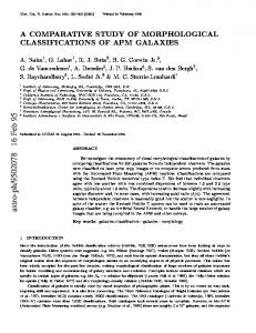
temperature data which were available from 1993 to 2011. Apparently, the performances of all proposed HBMO models, eq. (16-19), are different during training as well as validation phases. Based on the performance criteria, which are presented in Table 2, the proposed model that consists of four antecedent discharge data in the input has the smallest value of the RMSE as well as higher value of R2 and correlation coefficient in the training as well as verification period; thus, it is used as the main model for forecasting the river discharge in this study. As can be seen in Table 2, the model’s accuracy slightly improves with increasing number of antecedent flow. Most values of the RMSE, correlation coefficient and R2 has a limited variation range around 26, 0.9 and 0.84, respectively. As expected, the results of sensitivity analysis on parameters show that recommended model exhibits significant sensitivity to one antecedent daily discharges and average daily precipitation [33]. The best-fit model performance indicators RMSE, correlation coefficient and R2 have values within the ranges 18.05–32.24, 0.86–0.96 and 0.6–0.89, respectively. Consequently, after a comprehensive comparison between the HBMO and SVR models, this main model structure is selected as the most efficient model. The results which are summarized in Table 3 indicate that the HBMO model performed a bit better than the SVR model as well. Figure 3 illustrates the hydrograph and scatter plot of both the observed data and the predicted values obtained using the HBMO model for the verification set. Figure 4 illustrates the output results for the validation period obtained from the SVR model. As can be seen, the HBMO estimates are closer to the corresponding observed discharge values than those of the SVR model. Furthermore, despite greater RMSE values than the calibration set, the performance for the verification set is proved to be robust, Based on an error analysis of the calibration and validation set, it can be concluded that the predicted discharge during the high stream flow conditions are underestimated for a certain period. However, model has proved its capability of achieving the flood peaks successfully. In conclusion, the HBMO and SVM models display significant forecasting performance and can be appropriately applied for daily flow prediction. However, the results confirmed that the HBMO method has a relatively higher efficiency and accuracy in predicting the river discharge than the SVR method. Table 1. HBMO coefficients Variables Model ß1
ß2
ß3
ß4
ß5
ß6
ß7
ß8
Eq. 13
1.806
0.865
0.150
0.312
0.680
0.588
0.667
1.580
Eq. 14
1.464 8 1.288 6
0.890 9 0.911 1
0.470 6 0.019 7
0.648
0.119 3 0.506 6
0.164 7 0.729 2
1.087 1 0.014 6
0.461 6 0.701 4
21.09
50.93
-0.045
-0.155
0.334
0.566
0.733
Eq. 15 Eq. 16
1.076 7 0.237
10
ß9
ß10
0.648
1.590
1.654 9 -0.162
0.312 6 0.14
ß11
ß12
0.647
1.591
-1.279
0.317
ß13
ß14
0.6
1.5
8
8
International Conference on Civil Engineering Architecture and urban infrastructure 29-30 July 2015, Tabriz, Iran
Table 2. The performance statistics of the HBMO with different parameters. Training
Model
verification
RMSE(m3/s)
R2
C. C.
RMSE(m3/s)
R2
C. C.
Eq. 13
18.68
0.75
0.69
26.8
0.83
0.91
Eq. 14
18.44
0.76
0.86
26.81
0.83
0.88
Eq. 15
18.23
0.74
0.85
26.66
0.84
0.9
Eq. 16
18.05
0.75
0.86
26.45
0.84
0.91
Table 3. The performance statistics of the HBMO and SVR. Training
Model HBMO SVR
verification
RMSE(m3/s)
R2
C. C.
RMSE(m3/s)
R2
C. C.
18.05 26.17
0.75 0.89
0.86 0.96
26.45 32.24
0.84 0.6
0.91 0.89
500 500
Q(observed) Q(predicted)
450 400
400
350
Discharge(m3/s)
300
QObserved(m3/s)
300
250 200
200
150 100
100
50 0
0 0
100
200
300
400
1
500
301
601
901
1201
time(day)
QPredicted(m3/s)
Figure 3. The observed and predicted discharge by HBMO in the verification set. 11
International Conference on Civil Engineering Architecture and urban infrastructure 29-30 July 2015, Tabriz, Iran
400 Q(observed) Q(predicted)
350
500
300
Discharge(m3/s)
QObserved(m3/s)
400
300
200
250 200 150 100
100
50 0
0 0
100
200 300 QPredicted(m3/s)
400
1
500
301
601
901
1201
time(day)
Figure 4. The observed and predicted discharge by SVR in the verification set.
5. Conclusions In this study, an attempt is made to compare the capability and effectiveness of the HBMO and SVR models for daily discharge prediction. The same climatological and geographical data are applied for both the HBMO and SVR models in order to maintain robustness of the comparison approach. In order to achieve this goal, the Kashkan River located in the Lorestan province of Iran is chosen as the case study. The results of HBMO and SVR models and observed discharge are used and evaluated based on their training and verification performance. According to the results, the model which consists of four antecedent discharges is chosen as the best fit forecasting model. Comparative analysis of the performance criteria indicates that the HBMO model values of R2 and correlation coefficient are higher than those of SVR model. Besides, the HBMO model has lower RMSE values than the SVR model. It is worthwhile to note that the models with four antecedent discharge parameters are trained to find out the sensitivity of physiographical factors. Basically, the one antecedent discharge dominated the accuracy of river discharge estimation. The validation results display that the HBMO models have a relatively better capability of estimating flood discharge than the SVR model. In future work, we strongly suggest that it is necessary to include more predictors such as local rainfall, relative humidity and climate indices as the model inputs.
12
International Conference on Civil Engineering Architecture and urban infrastructure 29-30 July 2015, Tabriz, Iran
References [1] Kerh T, Lee CS. Neural networks forecasting of flood discharge at an unmeasured station using river upstream information. Advances in Engineering Software; 37: 533–543, 2006. [2] Aqil M, Kita I, Yano A, Nishiyama S. A comparative study of artificial neural networks and neuro-fuzzy in continuous modeling of the daily and hourly behavior of runoff. Journal of hydrology; 337: 22–34, 2007. [3] Chau KW, Wu CL, Li YS. Comparison of several flood forecasting models in Yangtze River. Journal of hydraulic engineering, ASCE; 10: 485–491, 2005. [4] Nayak PC, Sudheer KP, Rangan DM, Ramasastri KS. Short-term flood forecasting with a neur fuzzy model. Water Resources Research; 41: 2517–2530, 2005. [5] Wu CL, Chau KW, Li YS. Predicting monthly stream flow using data-driven models coupled with datapreprocessing techniques. Water Resources Research; 45, W08432, 2009. [6] He Z, Wen X, Liu H, Du J. A comparative study of artificial neural network, adaptive neuro fuzzy inference system and support vector machine for forecasting river flow in the semiarid mountain region. Journal of hydrology; 509, 379–386, 2014. [7] Kisi O, Cimen M. A wavelet-support vector machine conjunction model for monthly stream flow forecasting. Journal of hydrology; 399: 132–140, 2011. [8] Vapnik V. The Nature of Statistical Learning Theory. Springer Verlag, New York, USA, 1995. [9] Yu PS, Chen ST, Chang IF. Support vector regression for real-time flood stage forecasting. Journal of hydrology; 328(3–4): 704–716, 2006. [10] Wu MC, Lin GF, Lin HY. Improving the forecasts of extreme stream flow by support vector regression with the data extracted by self-organizing map. Hydrological Processes; 28: 386-397, 2012. [11] Lin JY, Cheng CT, Chau KW. Using support vector machines for long-term discharge prediction. Hydrological Sciences Journal; 51(4): 599–612, 2006. [12] Liong S, Sivapragasam C. Flood stage forecasting with support vector machines. Journal of the American Water Resources Association; 38 (1): 173–186, 2002. [13] Bray M, Han D. Identification of support vector machines for runoff modeling. Journal of Hydroinformatics; 6(4): 265–280, 2004. [14] Jayawardena AW, Perera EDP, Zhu B, Amarasekara JD, Vereivalu V. A comparative study of fuzzy logic systems approach for river discharge Prediction. Journal of hydrology; 514: 85–101, 2014. [15] Liu Z, Zhou P, Chen G, Guo L. Evaluating a coupled discrete wavelet transform and support vector regression for daily and monthly stream flow forecasting. Journal of hydrology; 519: 2822-2831, 2014. [16] Kalteh AM. Monthly River flow forecasting using artificial neural network and support vector regression models coupled with wavelet transform. Computers & Geosciences; 54: 1–8, 2013. [17] Afshar A, Bozog H, Marino MA, Adams BJ. 2007. Honey-bee mating optimization (HBMO) algorithm for optimal reservoir operation. Journal of Franklin Institute; 44(5): 452–62, 2007. [18] Niknam T. Application of honey-bee mating optimization on state estimation of a power distribution system including distributed generators. Journal of Zhejiang University Science; 9 (12): 1753–64, 2008.
13
International Conference on Civil Engineering Architecture and urban infrastructure 29-30 July 2015, Tabriz, Iran
[19] Niknam T, Olamaie J, Khorshidi R. A Hybrid Algorithm Based on HBMO and Fuzzy Set for Multi Objective Distribution Feeder Reconfiguration. Science China Technological Science; 4(2): 308–315, 2008. [20] Niazkar M, Afzali SH. Optimum design of lined channel sections. Water Resources Management; DOI 10.1007/s11269-015-0919-9; 29(6): 1921-1932, 2015. [21] Niazkar M, Afzali SH, Assessment of modified honey bee mating optimization for parameter estimation of nonlinear Muskingum models. Jounal of Hydrologic Engineering, ASCE; DOI. 10.1061/(ASCE)HE.1943-5584.0001028; 2014. [22] Jahromi ME, Afzali SH. Application of the HBMO approach to predict the total-sediment. Iranian Journal of Science and Technology-Transactions of Civil Engineering; 38(C1): 123-135, 2014. [23] Collobert R, Bengio S. SVM Torch: support vector machines for large-scale regression problems. The Journal of Machine Learning Research; 1: 143-160, 2001. [24] Maity R, Bhagwat PP, Bhatnagar A. Potential of support vector regression for prediction of monthly stream flow using endogenous property. Journal of hydrology; 24: 917–923, 2010. [25] Kao LJ, Chiu CC, Lu CJ, Yang JL. Integration of nonlinear independent component analysis and support vector regression for stock price forecasting. Journal of Computational Neuroscience; 99: 534–542, 2013. [26] Haykin S. Neural Networks: A comprehensive foundation. Fourth Indian Reprint. Pearson Education, Singapore, 2003. [27] Azamathulla HM, Wu FC. Support vector machine approach to for longitudinal dispersion coefficients in streams. Applied Soft Computing. 11, 2902–2905, 2011. [28] Hsu CW, Chang CC, Lin CJ. A Practical Guide to Support Vector Classification, 2010. . [29] Chang CC, Lin CJ. LIBSVM: .
A
Library
for
Support
Vector
Machines.
2001.
[30] Moritz RFA, Southwick EE. Bees as Super organisms. Springer, Berlin, Germany, 1992. [31] Omid B, Abbas A, Miguel A. Honey-bees mating optimization (HBMO) algorithm: A new heuristic approach for water resources optimization. Water Resources Management; 20: 661–680, 2006. [32] Olamaei J, Niknam T, Arefi SB. Distribution feeder reconfiguration for loss minimization based on modified honey bee mating optimization algorithm. Energy Procedia; 14: 304 – 311, 2012. [33] Foroozand H. 2012. Discharge prediction in rivers based on Honey-Bee Mating Optimization (HBMO) Algorithm, Case study: Kashkan river basin. MSc. Thesis. Shiraz University, Iran; 2012
14