A comparative study or Iterative and Noniteràtive

------------~~--------~----------------~-- , "

...

\

A comparative study or Iterative and Noniteràtive Faotor Analytic Teohnique. in Sma1l " to Hoderate Sam~le SiBes ,JI)

.1'

, , ,)

Carl G~ Brewer Department of Mathematics an~ Statistics McGi11 University M}Jntreal Auqust 1986

o

'A

Thesis supmi tted to the Facul ty of Graduate studies and Research in Partial FUlfillment -----., of the Requirements for the Degree of Kaster of Scienqe

" " ,

,

~

1 .. "

.

,~

.

,

-

"

1

L'autorisation- a ~tê accordêe Bibliothêque nationale du Can~da de microfilmer cet te thêse et de' pr@ter ou d'e vendre des exemplaires du film. >." (

Permission has been granted to the National Library of Canada to microfilm this thesis and to lend, or sell copies of the film ...

"

!. la

o

The author (copyr ight owner) h a s. r e s e r v e d . 0 the r publication rights,' and neither the thesis nor extensive extracts from it may be printed ,or ot.herwise ' reproduced without his/hef w rit t e n ,p e r mis , s ,ion •

ISBN

L'auteur (,titulaire du droit d'auteur) . se rêserve les autres droits de publication; ,ni la th~se ni de longs extraits de celle-ci. ne do i ven t être impr imês ou autreme,nt reproduits sans son autorisation êcrite.

0-315-34479_2

., ,

,

,'.

•

\

-_.

,

.

,

,'

,~

Iï~;,

,,' ,

...

,

,

,1

•

J Il

1

"

'v

'-

Il 0,

" • '"f_{

'

,

\\':

..._----

")

,

", 0,

:,ij

,

'f

,

---------~~

,

_-j\.U

,

, ,"

'II ~I

'1

,

"

, '

A

St~dy'

Comp~

,

'1

of Factor Analytic Techs.: ' Mad. Sample Sizes.

ta

in Sm.

,

Il'

') 1

l,

• '1 ~

Il

,

'(

,!

l,

\

Il',

1

\

.'

'

"

, 51

1

d

1

. ",

" J., 'l..

1

"-"

j,,,

'" ,

1 'II

II'

~

,

,,

'u

,

~,

"

"

,

"""

"

," "

",

1

.'

o

,

1

.'

U'"'

Il

,t

,

"

j

l,

",

Il'

Lt

~;,

",

.1

"

l

"

,

"

",1

"',

"

0,

"

, '"

•

,II

,

.

,

;11

,

,,

.

"

,

:

':

,

Il

"

,

"

,1 'e

,

[

1

, ,,"

-

,n

pi;

~ l

.........---- ..

',11

',"~

",

,"

"

,j

y, g'

f'

"

, "

"

"

,

'l

,

,

", ,

!'

, ~

, ,

,

"

"

"

'

,

"

~ Comparative Study of Iterative! a~dl Noniterative ' c

'

\

'

o

" ' 'Factor Analytic Techniques' in Small , ' . to Moderate S'ample' Siz'es

,

,

0'

"

.

,

.

,

1

, ,

.

.'

"

.

"

o -

"

,~,

Iii

, Carl G. Brewer o ' ',1

,

1

l

J

,j

, '

"

'

\ 1

,

,. "

'

,

1

, - 2 variables was set forth by G.U." Yule in lé ~897,

and was appropriately named the multiple correlation

coefficient. , The multiple correlation coefficient is essentially a

~easu!e

of the,strength of the relationship between a random

variable and a set of predictor variables. The square, known as the coefficient of multiple determination, is a measure of the , amount of variation f in a ,random variableoe,xplained by the pre-

Il"

4

1"

l

'

Il

~

01

o

dictor variables. However, the 'correlation coefficient leaves one question unanswered:

..

If the correlation coefficient admits the

existence of a relationship between a pair of random variables, what then is responsible for this relationship? The answer may lie in isolating a third random variable, called a factor, that is responsible for creating a relationship between observed or manifest variables. nistorically, Spearman(1904), was the first to

dev~lop

a

(

model based on the

~bove

concept. Spearman's data consisted of

"

test scores obtained by 36 boys on 6 different academic subjects. The latter can be regarded as the

manifes~variables

while their

ïnterrelationship as that being caused by sorne latent variable or factor. Moreover, Spearman believed that a boy's performance on a particular test consisted of two parts: the first a general ability factor common to all tests and a second more specifie, factor unique to a given test. From this follows that the more intelligent a boy is the more likely he is to perforrn well on all tests. However, two boys of equal intelligence may not score identically 'on a given test if their specifie abilities differ. This assumes that the general ability factor is uncorrelated with the specific ability factor. Spearman translated his ideas into the following equation;

o -- ...... ~

'[

\

, " 1

"

"

,

t,

X

st

==

,

+

X,

Il

,

H' ,

,U

"

0)'

'1

"

~ X 1

6 X 1

6 X 1

:1 '

'

\

" where

is a' vector containing as elements thte manifest

,Î,

variables, and g , ls a veetor eontaining the weights whlch measure" 1

--

'\

/1

u

'

the degree in whieh the 'general àb~lity factor le contrlbutes to"

,

1

the eorresponding manifest variable.

y is a ,veçtor un-_

F~na11y,

_J.~_"'-'

"

eorrelated with X which eantains as" élements the abi1ity variables specifie to X. "

Without 10ss of generality, we may aS,sume that E'(Y)"~"

=

E(X)

= 'Q.

0, and E(Y)

The variable X is latent and

e~n

"

0,

be aè-

sumed to have Var (X) = 1. Each e1ement of U is specifie to a eor-

.

" '

" ,responding e1ement of l, so that .cov(Z,!!) =

E(YUT )

,

i~ a diagonal "

,

matrix. This supports the fa'et that no specifie variable covaries with "an element of l to wpieh It does

not,eorrespon~. 'l'

:Furthermore; ,

'E(X!lTf = E[ (sX + Il>UT ]

-,

"

,

,

~

'1

~

() Il

J,

J

,J

l'

" ,

,= E[ ~xyT +

"

:

UUT ,]

1,',

Il

Il

1

Il

i "

"

,

',;,:

'II

'l,

,

l' b

,

"

, '

i

,

., " ::

"

~...

t',

1 1

/

~

Y

1 1

"

l,' l

.1')

t

'

, , ':" ':: ;:: ," : .'! :, ,,'

'

,

,

,r.:.

'J

J

,

,

J

~

.

L~

,0

,

'Q

'

"" ",

~

.,

'1

J l~

--sinee X and Il are

e

0

Il

, "" '1

'l, li

•

t)

, ~

)

6

•

,

d

,

[1

,

, l'

~

f

,

,~

1

"

" \

1

,

.

JI

,

1

,"

J'"

,,

Il ,,

.

,

';

/'''1'

,, "

j

1,0 t

"

;.'

,~'

l

~

J;,

L

,~y

,

.2.'"

J (

\

tI

L

~

1

"

~

) 'IJ

,

u

"lnatr~x,

t

1)

l

II

li

"'

U

r

J

"

B'

"

un~"Orr~l~te~. ,( ~~,; E CmJ:'r) ,,\:i~ :a di,aqonal ~

l

J

Il

~

and :thereforee thé,

1

t

, diff~jrEmt ' SPêlC;ifi'c, variables "'do" not cOV,8ry. ,Th~~ cova,l!"iélnce matrix ~

,1

1:,

,/1:

'!

li

if

l

L

'

,~

1

)",

J

11

L "

G

Il

l '

,'"

,~

r

o

0

"

u

,,

l

L,

'"

(~

l,

0

1

ij,

J

U l

'

~

'\"-1' ", '.

1

J i l l

'of ,v is·1· ...

r

,

,

"

1 "

, J,

"

, li

l

1

,,

,'

, ,,

Il,

, ,:J

," ',1'" IJ'

j.l.l

",

",

",

)

li

,

~ "~

i'

~b

,i

l

f.,

0

li

II, ~.J,

tJ

"

"

li

j

"

: l

,

'

(~',

t

' ~~ 'if

1

,11

l

t

'

~ ~

•

1

,

j ,

iflri' th~t·

"The assumption ,associated with this mode l,

.

",

~X4entifioation (Rotational J:nvariance) ,':,,:", ,"i ,J

t

~

"(2) ,

hplds

1

for a:hypothetical population and' that the observed d~t~ cor~ 1

- , $ f '

~

respond~,' L,

:';0 a sample of individuals from this population. The /1

,param~ters'

oC

f

1

,

in the 'model are the façtor loadings

.,

~nd 'th~' uniq~e'

1 JI l ' r

'

".

"

,

\

,

"

•

, '

variances. In practice these-are the quantities that are esti~~ted 'from a body of sample da~a. However, in order to obtain

consistent estimates of

the mo.del must

be identified. In other words, for a ftxed number of factors k,

,1

,

the-~opulation,parameters,

'l",

",

':",' is' there a unique péid,r, G nonsingular and of tank k, and Vu posi"'''' f ',1" , tl.ve definite satisfying (2). 1 ~( ,

1

•

, 1

"

,

The first step is to

!,

d~te:rmine

whether or not a solution

,

':'exists'~" ~ Recall that ~GT is positive semidefinite and of rank k. j \ , 1J

•

}ht~,'1

1

" \

jt

H~,~e, ~_solution ~lsts if and only i~ Vy '- Vu is positive semi,

,

r~l)k k. "

definite and of ~

~

)

1

, Assume, that, 'a unique Vu satisfying the , ;

.

·a~ove

~

condition

:'

'"

exi~ts. The problern is now reduced to the identification of G. Il , For '~, == ,1, '. the;' problern is trivial ~'. The' p equations; \.. l' . () ,\.

t

l,

,'\

'f,

, ,1

""I! l"

l,

l

,

"

't-

.

J

f~

-

'-

o

,

,

'

"

, \

or,

y

~

~'.'

1 '1

,

(3)

fr.:", !t.;= ~Z ,

\

~

+.cU

y i= GZ

f

"

conta~n' 'ex,;q~ly p unknowns, and t:herefore have a unique solution. Ill'

:If G is repla'oed , }) "

bY

,

-G, and

.z.

by "":.,Z,,

",

then the above equations are

,-

also satisf,led .. ' liowever such, sign changes are trivial and will be ignored whEm':d.ist:u~sing the uniqueness of solutions. , "

,

For cases in which k > 1'difflculties in identifyingoQ are

quickly encountered, sinee (3) ',consists of p equations in pk

0,

17

,

J

-'-

c

c

unknowns. The syste~ has infinitely'many solutions G for every

l - Il., For instance, assume t,hat the pair (G,ll> solves (3) exactly. Qpon makinq the fol l'owinq , transformations;

Z = QZ*

0

\..

, ..

ci = G*(JT i't is apparent'that (G* ,1Ùal'so .'

" ,

1

","i~h QTg ,= I,

sol~es (3):'

v =

• .A.

GZ + U

r--

, ," ,

,

"

.,

1

..

.

.

'.

.,·Vy = GaT t VU ., .

t

,

'. "

0

,

• !

'..

. ,

,' ,

"

. l

li

1

,

"

, ,, ~oreover,

/

= G*Z* + Il

~

,

\

" .

. "

H

d ..

,

\

•

'

, ,"

.

, ".'

~

r

J \

~hus,

1

'1

~

Il

, I

J ,

.

J

the postmu,ltiplicaj:iono .of,.the,'~factor l,oading m~trix by an

, ..

,

0

,,

"

la "-

,10'

,

............

o

-

orthogonal matrix Q results in a new solution for both (2) and (3). This is called the problem of rotation. A method of resolving the problem of rotation i5 to

imposeo~

diagonalization condition . .. The matrix Vu is assumed to be positive definite. The pre and postmultiplication of Vy - Vu by,the positive square,root of Vu-l.

yields; , "" V -1/2V V -1/2 - V -1/2 v V -1/2 u yu u uu

Q

The matrix Vy *

-

= Vy * -

l

,

l is symmetric, of rank k, and is the scal-

"

ed covariance matrix of the p man'ifest. variables. It may be decomposed in the following manner; VY*

-

l

= BDBT

where D is a diagonal matrix of order k, containing as elements,

~\

the k non zero latent roots of Vy * - l, and B is an orthogonal

)

matrix of order p x k, containing as columns, the k corresponding

/

unit latent vectors. Assume that the k roots are positive, unique, and arranged in strictly decreasing order of magnitude. The importance of this assumption will become more apparent in

o

19

.,

.1

,

,

'

,

•

'\)

,

Il'1

,, ,

~

p

ë~at>t'er',

~:

"

! :

'

.,

,.

f

~

(j

"

.

,

" ù

1

,X) V.u'1/2

,,

1 "

.

,

v~,1/2BOll1'Vu 1/2

, : ; : 'f

r ,u

..

r

M

,

," Il

,

(~Ul~2SD1 0, the number 1

,eq~ations

of

exceeds the number of unknowns, and only in rare in-

/'/

, stances will a' solution for Vu existe 1

../ Reiersel (1950) showed that, if a suiti.able u~ique Vu exists - '1.

fot k = k*, then infinitely many Vu exist for k

= k*

+ 1. Ander-

1

sop and Rubin(1956) have given a number of necessary conditions l

,

~

and surficient conditions for the uniqueness of VU. However these theorems do not readily lend themselves to the application of factor analysis. other conditions have been developed, but have (

also been found too difficult to verify in a

prac~ical

situation.

Furthermore, only necessary or sufficient conditions have been J given for the identification of VUI but necessary and sufficient conditions are unknown in general. In an effort to

~evelop

a set of conditions more readily ap-

plicable to factor analysis, Joreskog(1963) developed the Image Factor Analvsis model. The description of this model ls found in section 2.9.

22

•

o

2.6

"

Hultinormality and Factor Analysis

\.

So far ,the discussion has been limited to the case in which ~

and y are random

vecto~s.

The analysis has been restricted,to li'-

the first and second order properties of these vectors.' No assumption has been made about their distribution. In Many instances,

parti~ularly

---- - eswhen deriving maximum likelihood •

timates of the population parameters, it is useful to make the following assumption;

N(Q,:I)

Z

and,

.#

Based on the,above assùmption"x also has a multivariate nor~ mal distribution. The fixed factor model assumes that y i5 a random vector but treats Z as a nonrandom quantity that varies frpm one individual to another. Under this aS5umption the model is more" appropriately written

aSi

,

= where, ,k

= 1,2, ••• ,N

denotes the k th individual in the study. The

following assumptions also ,

o

"

~old;

23

I:}

•

~-

,

1

>

o

,

N _-)

(l/N>2:.z.k =' Q

,'\

, 1

k=1

1

;

, '

N

( l/N>2:Z.k.z.kT = l k=1 The Z-k are incidental parameters, since they only affect the manifest variables correspondlng to thé kth individual. This o

,

model in analogy with the fixed variance, is

appropri~te

eff~cts

'

models of analysis of

when the, sUbjectJ' in th; study are o(

interest. In the former definition of the model the subjects were regarded as a random sample of- individuals from sorne population on which inference is to be made. The expectation of the nonrandom factor analysis model ls' ,

1

\

and ls viewed as

~he

conditional mean of Y for ,a given Z. The

difficulty associated with this model is that lts likelihood ;

function does not have a bounded maximum (Anderson and RUbin, 1956) •

The random factor modèl with the normal assumption will be the basls of this study. Although the normal assumption is not 'crucial in much of the theory that follows, it will be necessary in the construction of random matrices. The technique for constructing these matrices will be discussed in chapter 4 •

•

24

•

,

,

Partial Correlation and Waotor ADalysis

Factor analysis can be viewed in terms of the theory of partial correlation. To demonstrate this

~elationship

a

defini~ion

,

of partial correlation is required. J

.1

J

Definition: ,Let Yi and Yj be any two random variableS-.J..n_,-a_random, vector ï. of order p, and let the random vector 1 co'nsist of k variables. FUrthermore, let;

be the least squares linear regression of Yi and Yj.on 1. The 'partial correlation between Yi and Yj ,aft~r the eliminatio'n

of Z-

ia defined as the ,correlation between Ui and UjOJ In matrix' form this is;

1 = 01. + 11

, ,

Q

where G is of order p x k. The partial correlation matrix of ï after elimination

~f

1 is defined as the correlation, matrix of y.

Recall that in the least squares reqression of ï. on "

regression matrix iSJ

25

~

the

"

." _

G

=- Vys"S

-1 ,

, where,

E

"

, '

l'

,.

j

1

1

""--

\1 J

1"

,

l

,,~~'

11t.:'t

1, l

.' ,

~;

'

j

, ,

,{

l ,

t

l,

" '

variable~' ~a'~isf,y!riCJ the .... ,

'

1

independent variables 'are, in general, co~~elated, whereas in ,

factor analysis the uniqu,e parts of the martifest variables are. , .

assumed uncorrelated by definition. ln spite of the contrast, 'the_' ') J • " t

multiple

corr~lation

~'

,

definition of the unique variancès has been j: "

adapt,ed to facto'r analysis, and is

'of

-

~

l

'

partic~t,ar importan~e 'i~ ~

J,

t

'Il,

Image Factor Analysis (ItA). The formulation '

.

.

cii

,

'1

the IFA model is , ,

'

based on a th$orem relÇlt~ng the ,residù{ll yariimces tQ the uni~ue

1

1

variances. In order to pres,ent this theorem a number of fact.s, , , '

about' multiple correlation \ will be stated.' c' , l ~

n,

.

-' . "

, "

'

~

].:

" ,'

\',

"The followLng equalities hold (Mulaik" 1972);

'1

'If

".

,

, ,

""

",'

, ' , .

1

o

\'"

,

o' \!"

,\

l'

,

,

1

-

,

'

'29 !

'

: ' following s,et {Y11 •• "Yj-l'Yj+l/ ••• (Yp} ~Y Rj:12 .... f-l·,j+1..'.p.,"

1

(t

9"

t

, ,

i'

•

\

Denote the multiple co,rrelation q~ ~ varia'bl~ Yj and the

, 1

t

c

,'. "

,

~

. ","

,/, ,

,

"

,

",

1

-~--------;---~

......... --

,"

,

"

.;

,

"

, ,

, "2

l

" ,

"

1

R j: 12' ••• j~~', j+1~ .,. P = ,

,

,

,

,

,1

,,'

(,

where Ivy'f is the detè~i~êj\nt of the covariance matrix of X, "and

t~e aete~inant Of:'":~Àe ~ovariance

1Vjj 1 is

matrix of

tb~ ~et

vj,~.'i,s the'jth di'agonal element of'the

(Y11."'Yj-l'Yj+lt""'Y'p)'

ma t r i x Vy - 1.''

,

'X'

The residqal variance is l,~ R 2 j:12 ••• j-l,j+l, ••• p 1/vj j . Let;

,

" , , ,

,

,

1
)'

'

'2

"1

R j:12' ••• J-l,j+1., ••• ,p ==

. ,, ,

(1 -

2

'2

r jCO> (1 ~ r jCl:CO) 2

,

"

r jCp-l:cqCl ••• Cp-2):

•

"

,

.

..,.

,

,

,

c

,

c'

,

.

,

where r 2,jCp-l:COCl., . ' iB the partial correlation •• Cp-2 Y Cp - 1

after 'elimination of

YCO'~C1;.

0

.~YCp-2. Co

0

,

f y j and

,may assume ,any

1

value in the set {j}C, Cl may assume any value in the set {j, Co} c, etc. Letting j ~ l, a' particiÙar realization of the , j

above

equ~tion

is;

1 - R 2 1:23.0 , "

x .' ,

,

,,

2 op = (1 - r212) (l - r 13"' •• 2)

(1 -

"2 ~, 14: 23)

••

' 0

(1

. Two conclusions may be drawn as a result.of the àboVoe

;

equations:

(1) A mUltiple correlation coefficient is never less than,the absolute value of à'ny correlation between an independent and dependent variable.

(2) Adding a new variable to the set of independent variables .

will increase or leave the same·the multiple correlation coeffio

•

cient between the dependent and independent var1ables.

"

,

32

\'

,-

•

Proof of' (1):

Since 0 5 r 2 !i 1 then:

.

.

2 1- - R2j' "~1' " :12 ••• )- ,J+ l , ••• ,p :S 1 - r jCO

or "

2 R j:12 ••• J-l,)+1, •• ..• ,p

.

jo'

R' ' j , ,J : 12. •• j -1,

~ r 2 "co J

+l, ••. , p

Proof of (2):

'),. - R2j ' ••• ,p , :12 .... j -l, j-f;l,

=

,(1 - r

2

jCO) (1 - r 2 jCl:CO)

0,

1'0,

= l - 'R2 ):12 ' l , '••• ,p,p+ l • .•. j -1,)+

('

Thus,

2• ' .)-1,)+ . 1 ,~ •• ,p •R ):12 •••

33

5

R2 •

. J : 12 ••• )• -1, ) + 1, ••• , p, p+ l

(

f

The theorem is now presented. ,

THEOREM:

The square of the multiple correlation coefficient

for predicting a variable

~

from the n-l other variables is a

lower bound to the communality of variable j. This is given by;

2 R 2 J:12 . .. ••• )-1,J+l, ••• ,p S h·J ,

The following proof is due to Mulaik(1972).

.

Construct the matrix K based upon the

"

matri~es"~y,G,

J

,

and Ik'

such that;

,

!

'

'-

Define a matrix,

such that IH*I

= 1.

H

*,

Thus,the matrix;

\ "

34

'C'.

,

' ,

"

, ,,

,

,

,

" ~

, '

0*

,-

1

J +~ t ,1

Il'

u '

"

"

,,

'

Il le'.

,

,

t

,,

F

,,

GGT

0

, '!

"

,

"

G

Ik

) ,

., ,,

'

..

, J,' l,

,

c y

" ,

\

(VU . ,

,

=

',0 ,f

G)

,(5)

Ik

is such that IHH*,I = IHIIH*I = IHI: wtiich follows since H and H* a+e square matrices of order p + k. ,"Furthermore, it follows from (5);

Therefore, it ,is cle,ar that;

IHI

=

IVul = u 1 2u 2 2 ••. up 2

where u 12 , u2 2 , •. : 1 u p 2_ ,are the diagonal elements of Vu' Moreover, let Hjj be a minor of H, and therefore of Vu' it is immediately apparent that;

, t

•

..... - -

,

, -'-

,~

35

'

f

~~-----------------------~~---------

\ ,

'.

1,

•

0

\

2 / R j:1.2 ••·.j-1.,j+ -,.~,Zp .; ,

,

= 1. -

= 1.

(1 1/ 1Bj j

1)

- Uj2

As a by product of this proof it follows that the multiple correlation between the independent variable Yj and the set ('i1,'i2, •.. ,'ij-l,'ij+l/ ..• ,Yp,Zl,Z2/""Zk) is equal to the com-

munality of manifest variable Yj' Applying result (2) of the previous page it follows that; r

R 2 ):12 , " ••• )-1,)+1, •••

,p,Zl, ••. ,Zp

"

This implies that;'

2 R j:12 ••• j-1,j+1, ••• ,p

36

R2 , " c ):12 ••• )-1,)+1, ••• ,p

•

...' or

1 -

l,

R'2 .

. '• J:12 ••• J-l,)+1, ••• ,p

In generâl;

(6) .

r ,

2.9

specialized Uniqueness MOdels

In section 2.5 the conclusion was that G and 'Vu could only. ,

be identified under special conditions. Much of the concern

re~

volved around finding a suitable Vu which would leave Vy - Vu positive semidefinite and of rank k. If nurnerous Vu matrices sati&fied the above criterion th en the chosen rnatrix would leave Vy - Vu of minimum rank. This is simply an extension of the idea

presènted at the end of section 2.7, and of postulate 6. This is known as the minimum rank model. Nevertheless, even if the minimurn rank model were found, which is very difficult to do in general, the problem of whether Vu is uniquely determined remains.

' . /"

The indetfrninacy in Vu can be removed if the Vu

= cl

specificati~~

is mad . This is the model of Equal Residual Variances

(ERV). Much of the work

~ssociated

with this model is due to

Whittle(1952) and L~wley(1953). Howevet, the majo~difficulties of the ERV model are

o •

tha~

it is not scale invariant and that the

37

•

r.

assumption of equal uniquenesses is not realistic. Joreskog(1963)"improves .upon the ERV model by replacing the condition Vu

= cl

with;

(7)

,

This is the

~mage

Factor

'

Analy~is

(IFA) model. The model assumes

that Vy is invertible. This is consistent with,postulates 4-6 of the multiple factor analysis model. "

1

The IFA mOdel is based upon the premise that the unique

variances of the manifest variables are proportional to their residual variances. ~The residual variances are obtained as a result of a regression of each ,manifest variable on the remaining set of p-1 manifest variables. It follows

fro~

(6) and (7) that

the constant c is less than or equal to 1. The following theorems

THEOREM 1:

~ue

to Joreskog(1963) are presented.

If ï is a random vector with covariance matrix

Vy , positive definite, then the symmetric posïtive definite .'-

matrix;

,

1

i 1

v,y * is invariant under scale ~ransformations in the computatio~ of

•

38

X.

•

Proof: An arbitrary scale transformatIon may be

x= îl: "

r~presented

as;

,

1)

.J

where

ia an

It

arbitrar~

diagonal matrix.

'"

'0.

Thua,

Vx

, .'

= EeXXT)

~

= E'(J(ll,TK ) , 10

"

,

= KECUT)K

.'

,

"

"

,

1

~ence, ,

"

,

,

,

,'

1

J..

,

.

an4,

;

, ,

,"

';

,"

F1na11y,

\ , 1

•

v x * = Wx-1/2Vxx • -1/2

1

"

-,

l'

:. 39

~.

:

'-

f

)'; ~.'"

(1

1

,,

l'

\

"

"

'

"'

"

/

-

~

l

'"

'

.. '

l

, J

,,

\,j

.',

1

,

,

'

\

,"

•

= .-1/2" .-1/2Y

,'r

'

"

"

,

,','

f

\-,

.

~>

,

"

, "

,

=''vy,*

'

,

Q

,

.

"

"

where W is defined as in section 2.8.

, ,

' ,

~.,

.. ,

".,

'

.

, '

"

Let.l be a p component. i-a.rl(~olù . . veétor

THEOREM 2-:

~

'v

covariance matrix VY' . p,ositive definit$, sati's~~ing~," "

· '" . ' ..

.r

J

\ ~

l~ ~. "

.

"'

" "'

"

'

"

cw ,,'

~

, "

,

,

where G is'of order p x k (k '< p)

.

.

", ,

~ositive sea'lar.' Let' ~

\., \

t

J:

Q

,

~

,'

'vy *

.'

t

"',

1

~ ~ ~

r

( '

~

.

, ""

"~

'

"

'.

,

,

...

~

,

,

"

~ \

" prè',

1

-l .. ~}

.

'-.

1

'f I,l

?UC~d, to' ~he ' "

' "

'r

..

field of regression and correlatio'n, by Dwyèr in 1924. ~asically , , ,

,\li

"

,

the assump.tion is tbat the, weight ,vector 'der'ini:nq" ~h~, linear' ~a,-, bination i8 (00 •• ,.0

i

0

with',th~,1 in'the i th. po~ition.~ ,

.... 0),

, "

'

,

:.

'

The resul tinq factor loading ma~rix i~ lower" triangular. The centroid method of factoring is' ,attributed " Thurstone(1947). The choice of a, weiqht vector for

ta ,

th~s

0,

,1

,pat- , 1

ticular method i8 a vector of l ' s'. HOWEwer tbi,8 'choice ::may, 'some"'" times resu1t in a negative vari~nce for a :cert~in ,factor'.

TIÙs"

effect' is e1iminated by reflectinq ,sojne of :"~he, signs in th~

r~duced covariance matrix and 1.'" reestimating th~, varianb~~ , ~

,

, 1

"

·The principa~ axes method, ls ve'rY,' si~~lar ~o t~'e p~in'~ipal. _,.1

, "

56,

~;

, ' q'

, '

"

\

. ,

'

" , ,,

,

,

" l"

.

l'

,

..

'

i' ,ma'tr ix ~ , , '

1 1

, ,

','

l

"

"

l

, "

{'

,

. ~

~

'

1

(

,

"

,

,"

,

,

.'
These' 'àre' the methods cf'" '.".

l ' b ' "

Il

,

,

~O"d~1;:~~~~~t, mé~hc:>?~' pf f~'t~i~q :'~hk"m~~~,~x" 'Yy .t~

,

: '

'

"

~~." ,'L.~~t,',SctUares ,'prO'c'edU~~S' i~ 'Fact~r ,A~tüysis ,

,

. : ... '

"

),

"

,

,

,~\ ~

l

!

.

"

\

"

" ~,1

.:

1

"

..

1

l

,

,

1

,

"

"

,

,

,

,;,

.,

'

l

,

l

~

\

"

, ,-

Il .'-

'~!

',',

'

1 '\

,

,

" 1

.

,

"

,

Il,

'1

"

l'

"

,

,

'

.

'. {

,

,

,,\

1

l,

,

,

\' ,

01

"

\

"

'

'l.

\ 1

'

1

, t

"

\_,

\

1

'

1

•

1

t

\

,\'

,

~

\

, 1

"

'l'I

1

"

,

,

,

'./ , " :1

,

,,"

',1

\\

:,,, '",""< ',This

Il,

"

,: r

"

.,

,

, , \,'

i .

1

"

, ',,

, ,

t

'l,

l'

L 1

'

)

,

l

,

procedure' gives aIl. vÇlrrabl~s equa~ wèight. Th~ iriter.. \

~

j

fi"

,1

' ,

'\

1

\

l

,

,1

, , \

\

, , , : " pr.étation 'of' ULS, is 'the, \.taual '; the variance of the errer parts "of ~, ','

"l'

, " \

\

" \

\

t

''

'

\

1

',.' .

"

of

,(

•

"

\

: ....

,

'

\

\,

'

,

"

\

\

,,,

,,1 l'

,

•

\

."

~n

'

,

factor analYe;is i5' a mul" , " ,

Q

'

,

tpe id~lJtity: ·matri.x .. Hence', the diagonàlization condl-

\

'l'

,

l

'1

i~

simPlified to

.

.fi

~TG"

beipg a

' ••:",

"

,

~iaqon~l

:"

\

,

'


',\

1 • \,)

.' ,.1

r'

"

~

"

.

.'

, ,

"t

'.

,\','

'

l'

~\ , ~ "~',

LS

,',

l'·..'

~

, " Q ,

• "

.< .

L

l

'. '

,,

~

"

,

,1

"

l','

,

"

,

'

,,

",

)

,

,

,

,'~~'nQ~ be~~~~x:t th~ '~,~t~~'6es :8' an~.,vy,.i~ th~ ~ètri'c s,~,:~', Th~t, is:' .. " . .. , . , " . ,. " .' "'.:':'·':,·:'' The. fol1owing equations hold, due to the syrnrnetry of S - Vu; arid the standardB1 "'" n~l."" , 12k) ,

ization of the latent vectors:

, ,

=

D.

+ Furthermore,

D1 1/2»l TB l D l 1/2

=

Dl

= 'G T G 1

,

1

thus,

If al. oiT is -such' th~t the function ULS obtains its conditional minimum, then the 'following equation must be true:

,

ll,1

\

,

\

tr(B 1D1B1T ,+ 62

B2 D2B2T

f

',_ )

•

=

\

\ 1

,

1

l'

"

"

=

"

v

=

\

Since aIl the latent roots of S - Vu are nononegative and u~iq~e it follows that tr(D 2 2 ) is a minimum if and only if 02 cont~ins

the P .. k smallest latent roots of S - Vu. Thus, Dl

contain the k larges,t lateI)t

root~

m~st

of S - Vu' and G1 contains as

columns the k corresponding latent vectors. In conclusion, the conditional minimum of ULS is attained when the columns of Gare chosen as the k latent vectors corresponding·, to the largest latent roots of S - Vu. It is noted that if any one of the largest latent

root~

of

S - Vu is negative then the corresponding lat:nt vector will be, imaginary. Unfortunately, this event occurs quite often in , practice.

63

\

\

,

c

. The minimum of GLS with respect to G for a given Vu is

~ound

by first evaluating the total differential:

dG LS

= =

(1/2) d tr(s-l v Y - 1)2 1)2 (1/2) tr d(S-l Vy

= = =

tr[ (S-lVy - I) d(S-~Vy - I) ] tr[ (S-l Vy - I) S-ldVy ]

Thus,

= ==

tr(s-l vy

= =

2tr(s-l vy - I) S-lGdGT .

dGLS/dG

/

"-

I)S-lGdGT + tr(s-l vy - 1) a- 1 dGG T I)S-lGdGT + trdGGT (S-IV - 1)S-l y

2tr[s-l(vy - S)S-lGdGT ]

=

2S- 1 (Vy - S~~.-lG '>: ... ;,'}

/,

,The conditional minimum is found by solving:

,/ ,1

'.

2S- 1 (Vy - S) S_:-l G =

(Vy

-

S) S-IG

0

,

=

0

SS.f'-1 G =

V

G

=

64

\

s-lG Y

Va- 1G

y

/

1\

I)S-ld(GGT + Vu) ]

tr[ (S-lVy tr(s-l v y'

~

r 1

a

...

,

•

'

"1

, Using.this expression, the inverse of vy.may be expressed as: Vy - 1

=

(Vu + OOT)-l

= Vu - 1 , -

Vu-1G(X + GTVu-1G)-lGTVu-l

~'\... Substituting this formula into (2) yields: r

l

/.

/ ---

)

' 1

=

Vu -l G El

-

(I

+ qTVu -lG) -lGTvu-:-1G)'

By (3) it is clear that: [\' r l"

ThUS\

(2) may he written as:

.. =

=

o

65

( (~)

Recall that GTVU~lG ls a, diagonal matrix by the diagonalization coridition given in section 2.5. Hence, (4) is an 'eigenequation, and the elements of D = (I + ~TVu-lG)-l are,the latent roots of Vul/2s-1~ul/2. The eorresponding latent vectors are the columns of B = v u - 1/ 2G• ., Assume, as in section 2.5, that the nonzero elements of "

aTvu-1a are positive and distinct. Thus, D is a diagonal matrix with distinct positive elements less than or equal to 1. Sinee D

=

CI + BTB)-l, it follows that th~ latent vectors should be

..D9:tmalized so th'at;

..-r"

I..:..:J.

=

I.

Notice' that the elements of BTB are aIl positive. h

The question is: which of the p latent vectors of Vul/2s-1Vul/2 are to be chosen as the k columns of the factor loading matrix G? In other words, which k latent vectors will minimize the function GLS ? The principles of notation pertaining to Band D will be ex, actly as in the

ULS

case. Another rnatrix, B*, i5 introduced. Its

columns are the unit latent vectors of vul/2S-1Vul/2~ Note the \

following facts:

c

66

\

,

a"

•

\

=

B

B * (D -1 - I) 1/2

Bi =

B1*(~1-1 - 3:)1/2

B

8 *(D - 1 2 2

2

=:

. 3:)1/'2'

/

, !~

,/

(l'

, 1

G1

=r

VU1 / 2 Bl'

'!Ul/~B1" (1)1- 1 .- ,Ir 1/2

=

"

1 '

,....

-

If G1G1 T is such that the function GLS , 9btains LtS conditional minimum, then the following equation, mU,st be true:

,

1 1

where Vy1

=:

" G1G1T + Vu·

-

. (.

,

Note that, vu-l/2VYIVU~1/~

~', vu-l/2GlG1TVu-l/2 + l' ,

67 !

)

1

~n

..-o

,

,

•

./";

.

.

,

,

- \ ,

,

.

"

.

,,-:.

".

t :

"

,

.' l -

'. ~

...

•

-

-, ~

=

V' -1/2

, '_ y~ U

,U

D' *B 1fT - B *D ' B2*'~'" 2 2 2, 2

..

..- ' . (

,

,

V,1/2S"'1v.

.... "

1

.' \

'

Tlieret:or~,.

. .fg (~u),

==

~f '

"

.

.

t

,

"

\

'

-

,

-" . ,
'.

1"; 006

0~'333' -

~~

'CJ_-

~

".

,

--.... ---

\

---:>--:.=:.. - ~':.-'::'-

. ~~

.:__ ot.-~

1.000

1;


..J

t"f')

,

.J

III

,.....

'e

~

'1(

09°000000000

rt 0 It.

~I

'l'l,

,0$

•

..,"'

ry

T

.....

....llJ

0

... M l'ti ,.. 10 0 ,., ,.,.., ... ru 1\1 .n ln 0 on .0 '1'1 '1'1 ." ~ m,.. !Xl .n "1 "'1 0 ,.. ·n 0 ". l'ti C'llll ", ,n IOtrI"',.. ... IO ..... N,..tnUlo (II". O'II)(JI(II .... IT)mmmOl

,.-:r Z oc( (}

• •••••••••••

1

~

,

Il'

1 1

1 1

' l'Y

,, , ,., n

U ri

1

"''''''Zf·O !i'6,Lte.·0 OLSOe.·O l,1>U;'O e01>2f,'0 0;n26'0

1

EC9ÇE • 0

SIL2e·o l!:ESL·O ÇOt1>e.·o ,.Clle.·O €c-..l.E."O 2f6e6'O 2'ç Hif'O OSC9e.·0

~C::J"

"~NY~

bC::JH\

-----------------------------------------

s'n=OCH~3~

L.1:60·0 ;.tl1·0 1>6~ 1 t • 0 !ii9601'O

10.35101

SS9.0·0 ,0tliO'O 2.290·0 'ln.o ·0 SiSih'O '0 &96.0·0 1~6~0·0

sçel:o"o 625 ... 0'0 8.L9.0"0 8LL.0·0

LZ6 • .o·O

" .. s ..

90110·0 .1>610"0 91>roo·0 ,L6S00·0 99nO"0

~1"lO·O

9(".ZO·0 21900'0 90010'0 ezel0"0

:!i3SW

:!O::SI'i

SlEOO·O Z0110'0 "OÇl0"0 1>tS20·0 t6~;0·0

tito90·0 S.ÇOO·O 1.010·0 t'9.l.TO·0 .oroo·o LE'SOO'O ,,01'0·0

.:Iï::5W

çLole·o E6t>lO"0 6t120·0 6L510·0 "502'0'0

e:,,01e.·0 ... zeoe·o 00,,'·0 29to2f.·O

20600·0 C,t'10'0 Zi 1,0· 0 h':CO·O tSfOC·O 91910·0

o,,6,e'O 9LOt'(,"0 '9tole·o 02tre.·0 Sil."(6·0 t:l.t2'"0

29~ZC·0

......

(210'.0·0 CC2SiO'0 L0290·0 0"."0'0

.e •• o·o

lSi:lSiO·O 9(, •• 0'0 S ••• O·O 959.0'0 2SiO.0·0 ZtoSi.,·O ZZ~;O·O

"as ..

eee.oo·o 1.210:0 9S9tO·0 09L('0·0 S9t5iO·0 61.90'0 OSit:OO·O t.('10·0 6.1.610·0 92"00·0 e9900'0 SiC210·0 .;:r,~sw

T'Ç.l.~·C

SS~06·0

.1,10'0 6t:SlO·O L5Z,0'0 SLI.IO·O €lZ20·0 "oro·o OL Il C· 0 6t>91C·0 l~"ZO·O

1>.1.900·0 h01C·O 9rSl0'0

=C:O:SIoI

t'L6Çf'0 1 E'S: 1>f ·0

.L"t96·C tert>6 oc.

"c.~'e·o

"C't'f·C 9tÇ-ZE·C

ec~ze'c

rEs.t.~·c

U'C.1S·O

Cf-5Lf-'C E'l'ç.t.·C ,Ll,Lt'e'O 5 06f f ' C 521ft "0 t-Z\'9f ·C

1>E.l.~6·0

Ç'96S·0 6lCLe·0 " " l{;l;. 0 LEtrlit·O cr"E 9t: ° 0

""Nl'::

~C::ll\

=c::~w

l~=OCI_J.:a

...

LI60e-·0 COf:Of."O 9S90e"0

2Ç,,6€·C

C291t·O

2'12~·0

S., ... 1f·O

9t"50e·c ge5LI..·0 9.LtrOe·0

~c:nc

!:L.~e·o

,ftor u· c 512\>e"p 1

Cf. • C

l.1.Sa·c

t.~Ct:ç:·(I

~9Ç2f·O

.Leese·c C~C;Pf ··0 CflU·C

,soze·o

lE 9Sf • C

92.ge· 0 s"cç'e·c ~ oe. 2f • C ,09f:t ·C t!:L.l.f·C t-6fSit-·C·

p..jo,N'C':>

~c::~c

"o,e,,·c

fS~l~·O

E6Z1f.·O 9Se:Zt:·O

~C:>1\

------------------------------------------

~~=CCI_J.= ...

1_2».0 '0 80S;.. 0·0

9"L90·0

6~1!i0'O

'6CS;O·0

,5.90·0

v

"35 ..

E:C~OO·O

LIzro·o 001"10·0 e·cco·o S6090·0

e;t.l."·o

.,L.OO·O 5,110·0 C;~E t O' 0 stroo·o Ç.LÇOO·O ,0210'0 ='=5 ..

bEZIC'O 6C91C·0 61""C·0 -C;'.lC·O tt12C·0 9crro·c C'LCC· r5 ... 10·C

°

62"'C·O

ecçoc·o OC;., 1 C· 0

f_61C·O =Ci!S ..

11>O.l.E·0 20"1'6·0 1..6ë:C6"0 E9Lle·0

e",se·c

tL~eç;·o

9\H'PO

tOI'E·O eee2e·o CE:,oe·o 1C;SL"·O tSf:2e'C tolti:t·C e 9:

-CÇl CE

," (

C~

cçt C€ ct-

=-'c" \' S

.

ë.'

s~c .1~~

...

.

, ..

----------------------------------------- :o:, ... =cc~J.=" ------------------~::;~~~3;;-;.r~ ~~

f'l

\.1

'--.

alq13 1

~.~..

~

g

\'\. ;

f~'

,~.~

\

0

ri

0 )

Table

1.4

Ma"xwell's Data Fre~uencles b~

varlOUS categories of methods Image

MeasuT'e: Method

ORCOR

10,

1

Il

11-

CANMN

- "

Tor best performance

veOR

FactorAnalysi~

MSEOF

MSEV

MSEL.F

Total

"

1-

3

1

2

-~

13

19.0

l!

9

1"1

10

7

59

82.0

PCAMLE

,.

,

Measure: Method

ORCOR

CANMN

VeOR

RO

0

0

2

al

12

12

10

,

MSEOF"

Measure: Methocf

OReOR

CANMN

veOR

MSEV

0

1

1

1?

11

11

Iterative

'"

MSEL.F

"

Total 4 68

" -5: 5 94. 5

Methods

MSEOF '-

MSEL.F

MS EV '-

"Fatal

"

6

1

0

0

8

12

48.6 16.7

4

6

:3

25

34.7

ULS GLS

8

4

8

8

0

1

3

MLE

4

7

1

,

0

35

AlI Methods -, Measure: Method IO

OReOR

CANMN

VeOR

MSEOF

MSELF

MS EV

Total

"

. 1

0

0

1

2

3

7

9 .. 7

Il

10

9

7

8

10

4

48

66.7

RO

0

0

1

0

0

1

2

-2.8

RI

1

:2

:3

:3

0

2

11

15.3

0

0

0.0

ULS GLS MLE

0

0

0

0

0

0

0

1

b

0

2

:i

4.2

0

1

0

0

0

0

1

1.4

.

1

::.:

....~l...- ..

--

.-----..-----~-

.I'-I

o

o

Maxwells ~ata

«

2 Factors Extracted

ORTHOGONAL CORRELATION By Va,riou8' Sa.mple

S-i,ze-s

0.990

d.985

1-




_

.:- ~~

-~.


';.

>

,
-;'Y':,

~n .1 ;:

.'O.oJ.&~

,"

..

'.

,

"

".

Q'

"

O.OU,of

J'

UlS

'

'

i ;-~

.. ,., _ ' . '
'

C"

. t

'\

CQ~~.lation M~t~ix

:

--------------~---

J

~

\

".

t

1.00'0, 0.523

".

,"

1.0~O\·

' "1.009,

,

. ._

0.408

0.451"

0.~59

0.511

0.332

-\1.000-

,0.356

0.437

0.296

~''-687'

0.451

0.267

t . ,0\.79-2

,0.560

0.568

0.463

: ,O'~·44-0

6."35

0.294

0.6,.5

0.6_36

0.206 -., 0-.2a9: ... 1 o • 59_!:) ,,:O~~1-7'-_~

"::~~~-Hr\..-_ ~

;:.

"

_

~

~

~

\

~

-

\

\

....

~

l'

't ...

\'

9·353

0.384 -

1.000

Q~~t55

0.315"

0.382

O.41J-?-:. CL

-~

.-:c..

_ ...

..,"C.

~

~

0.465-

,~

1,.000 "" 9. 4 71

._-676

.;'

,.'

",

-\

"

T~

l-

~-

.::

." ~-

t

~

,

'-

...-

,"

.Table-, ,- 2. 2~: '-:=>-:~-~=: '--

• •••••••••••

... lI)en ... ,...I"I lIJ

000000000000

1 1

,

In ... fd (fi ., .0 ln

,.,,... ... NNCO.oCO OIN"'''' CD(\! .... -0 0> III c> 0 >()>O ct 0........... OO ...... oN ... O OOOOQOOOOOOO

1 1

1

1

,... ... o (7I(IINo() .. 000('\ '" ... ..,., ., .... 10 en In

'" III

2:

,

_.

IL

:>

10 1/)

• ••••••••••• 000000000000

J.

" ..... 010 ... 0' tO. "'.,,, "'."oON-""'''''''ON "'.""no .. l"lf\) Il''1)10''1

IL

_1

·..... , .....

~ ~~gg~~;;;;g g~gg

:.;'

hl II)

:l!:

1000000000000

, 1 1

t1 ~.

U

ft'

.... norl..-4I) ... -O~OO

"1 7.

000000000000

III

n

,,

• M

n hl

·...........

7.

OOOooorrooooo

1

~

0O

... cr

00"'1')000"00 ""'0(1"100(1""'011"""01)

...

...

•, ,, ,1 •• ,•1

, 1

IL 0

h'

CI)

X'

'II1'\t-1II .. -1II01O'" "'1') «Io-n- ... oOt-f'loO"'..,oc\ fl/VlI') ...... o()oIIOIlOnc. "'''0 "' ... 01 .. 0 0 " o n 0000001 0 0 0 0 0 0

"

.... ...... ~

00000

000000

.. ..,1/l"'0'"NI'101NCo() IIII/It- "''''0 Cl 11) . . ,.,,.. ...

Ir 0 V

>

"'0'" l'llO " ""0""'1'100 (1 W

00000000.,000

cr

~'n

~

,, ,

2:

0

'T

!" "

1/)

• ••••••••••• 000000000000

1II0","' ...... VI",NN"'. "',..., oOOOOO'CI.o-IIIO 10"'''100-0'''''''' CO,..,., ",NN 000000000000

1

, ,• f 1 1

> hl

000000000000

"'''',..0' t1f \JI .. " t-UlI/II/I ...... "'ofIo(),

~ C

R 0.965 N

o N J

"

,

C ft 0.980

':

l

...

C

o

ft ft

E

..-

o. 975o~" ~ ~ ~

L ft

-

,,~~

f'

",

~

T

1

a

"

0.970 ~,

0.965

"

"-'"

0.960 1j

ULS

..i

&LS

RD

"LE

tu

,

- [0

11

FAC10R AMALll1C PROCEDURE

,-

"SRttPLE

.......-. 40

........... BD

t!t"-t!Ht 160 '

Figure 2.1

. ":,.

J:i:.' •

,1': r,

o

~~--

o

---~~--~--~-"

,

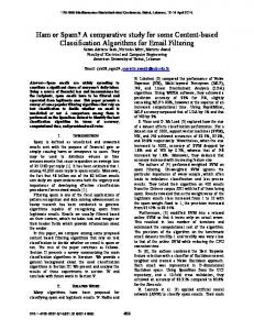
Em.met~ Data

-~-:;..--.-.-.~

'.

J.~~~~!

4 FQctors Extracted

CANONICAL CORRELATION By Va.rio1.l.8 S ample Siz es

G

0.99

"".f

0.98

l' ~-

C 0.9'7

A N

-

" M

) 0.96 C

A

l

C 0.95

"R 1

r.

R E L R T

,

1

"..

1

"\.

o. 9~

J-

o

H 0.93

0•. 92 \ \~

-"

o. 9J -1

i ULS

RD

. GlS

PILE

"

.~

")

~

Hl '

10

Il

FRCTon RNRLllJC PROCEDURE SAMPLE

.-.-. 40

.............. eo

~16D

Figure 2.2 \

Q.

~:

o

o EmmettS Data 3 Foctors Extracted

CORRELATION of UNIQUE VARIANCES By Va.rioUB Sample Size8

"'0.99

0.98 c

o 0.9? ft ft

E

L 0.96 A T

l ~ 0.95

"""

U H ) 0.94 Q

u

,,.?l', "

",~

- 1

~"i't''''''?'C' t

T..:

•

,

\

'o~

""

~

t

. Ha,.rr.fla:rYS

1.

,

..

hO.,

~.-'

)~ - ,

Factor Loading9 ,,160 .

' 187 ,

,689

-

.

.

-~-----~--------

"

,160

,>

'

.439

,096

: 780

>

570

,110

.644

.099

"

~27

.,080

',652

,219

.

18~

,150

,083

,137

-.019

: 233 ,739

'0

,. )

"

" '\

,

1

kIl

, ".

\

.

._~

:205

.2;33

,806

, 197

,075

.569

. 153 .242

.338

· 132

.293 .486

:806

.040

.201

.227

.257

0.168

.931

-. 118

· 167

.239

.180

. '512

. 120

,374

.551

,019

.716

.210

· Ô88

,435

, 198

.525

.438

: 082

'.4?0

.,197

.081

.OSO

.553 .:

.646

.122

.074

.116

.520

.696

•. 069

,062

,408

.525

.142

.219

.062

.574

,026

.336

.293

· 4~6

.

" . '93

. 148

,.161

.239

,762

'.378

. 118

402

· 36~ .301

.175

.438

.381

.223

.583

.366

.122

. 399

.301 .

.

.369

.244

.500

.239

.370

.496

.157

.304

~

.311

.066

-

\'

J

.352 ,

.767

~.

Î

'"

0

-!

-\

Unique VaT"iance9

;436

117

~

C'~

0 .

-----------~---

"r~

.".

Daia ,..

.... 1

!

.'

•

Q

"

.

~

;

\

\

.

,549

0

'

~99

\

591 ,601 0

{

.497 .500

Table 3.1 ,,"

,"

'" '"

,~

.::

T

1 : .1~',,:.rfV"';Y:~~~f{~~t;"'~' ,

"

1

'l'·

f

,

",'

,

l,

1

' .!

',\

,"

"

h,

, ""

,

\'

1 :

"

:'

"

"

,

1

"

" ' l,:'

:,

"

, ,

,

, , ,li, '

,,'l'

0' ,. l'

"

", "

"

','

~

1

l

. ,.

'.,

..

,0 \

.,

1

.'

'.

,

fil,

"

,',

,

"

," \

,

fOI,:'

...

,00

N

...

... 1

.. , .... 1

".

..

•

,. .."

"

•

o

0,0

0

tJi.,. •

1\1

,

- ... OP,'"

,..

N

...

;, .;

lic,

...a,,

•

Il,

;1

..

III

:,..

..

'"

~

;0

,. ... ... ... ,., • 0'4" o .,

0

"III' o 01, '0 .. o • ': ' 't.

, "

•

"

•

~

..

··I r: ... -::~ ~

,0

0

,:l,

,..

fil

fil

1\1

o

0

q'

", 1

.',

~

.. '0,,0

1'#,. ~

o .,

... 1 .. t

o

o

«) •

UI

0 1ft

01

fil .. 1111

PI' •

~ ~

~

o

~N

,.....

C"

00

fi

II'

;"0''; o

~

co ..... CIl

'"

o

0

fi

..

CI

N o

'" 0

... ......,

III

',

co

.,,,

o

Q

.0 . Il '>CI

>0 ...

'"

~

M,

"

"

0 1

.

"

:'H,'";; '" • • •.

fit

fit

~,

...

ft

.. 00

o .,

..

'

,

;

..

.. .0

0

"

,."

· '. ,. ::.. ',. ",. ..'" . .. • . '. · . . . ô .:, J ': ,: : : '" ... .,. .•. · • • • • • ·.. ·: :"". .::'~'. .'••

-', .,

,

"

\

0,

0,

Q '0'0

....

~,

','

:,,:' ., ,

o

.'

~

~.

0

!' co

. '. . .. ,:. fi,

.

.·.. ,'~iro/';/ ., 1.;'. =..,

.. .. III o "',0

PI

'

','

0

':

4>

....

... ! 'N

,"

'"

110

•• ore .,

,

"

"

o

•

,, , ,"

..

0, ..

., ,f\o • 00

~ 0 o

W"':' ....... ", .,c""

o o

:."

If'

:'

1

l,

~

,

~

~'

1·

•

..,

,'E-t' ", ~ "

,

"

,

0

~,

,1

'

,N

o

0' ...

'.-'.. o ...

o ..

,,.: ::,. ,.,~

••

• 0• 0• 0

0

~

"

0,0,

, ... ' ,

...

0

0

'.,

•

'"

......

.....

-

~

/ Ct

IV·

\'

\

~ ~" • ..

fi "

CI 1ft

~

'Z ':'

ft

..

.. 0

' .. 01 PI PI ..........

~, ~

': ': ':

" ~

'.

~

, .'

\

0

0

,.,

t·

.....

0

:

•

..

..

0

.. ; ;

ft,

':'':'' 000

..

.,

0

fi'

·.. ....fV-.,,,, . .... ..

•

0

0

0

,. "".,

• ft . . . . . . . . . . . . . .., ...... N 0

OOOOO.~O

1 f. .,. :

o

fil

... 0 •

-

fil

..

co

CIl

..

••••

'.

CIl

:

-... .: 0

..

pt

0

0 fil

",

l'V

0

0

0

-0

.,

.,

'"

...

fV

0

0

...•

o

0

o

0

•

.,

CI

••

fW

..

o

,..

". '" "' '"

d~oo,